Integration Project Systems and Control 2013 Group 3: Difference between revisions
Jump to navigation
Jump to search
| Line 252: | Line 252: | ||
{| | {| | ||
| - Improve the results of FRF measurements by applying new identification methods of course 5MB40-system identification. | | - Improve the results of FRF measurements by applying new identification methods of course 5MB40-system identification. | ||
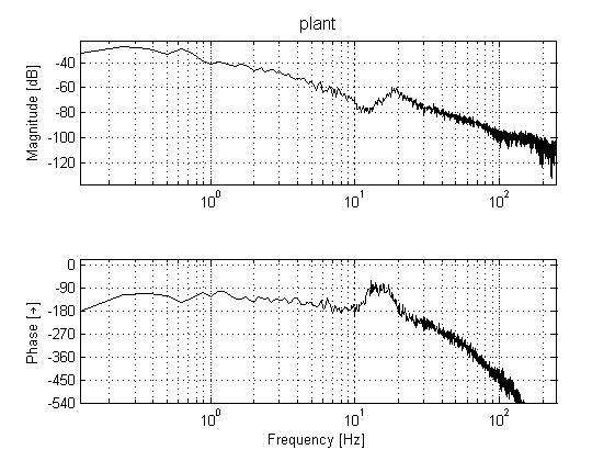
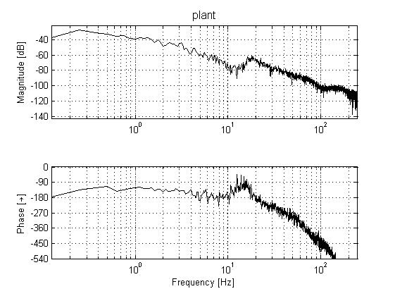
| - As our initial plan states, we scheduled to do our FRF measurements by closing the loop with negative feedback on each axis, thus stabilizing it (with a low bandwidth controller), and then estimating the frequency response by using the three-point FRF method. We were able to get an acceptable FRF on the first axis (the vertical movement), however on the other three axes our results were unsatisfactory, with the main problem being the high noise making the gain and phase estimations unclear. | | - As our initial plan states, we scheduled to do our FRF measurements by closing the loop with negative feedback on each axis, thus stabilizing |it (with a low bandwidth controller), and then estimating the frequency response by using the three-point FRF method. We were able to get an |acceptable FRF on the first axis (the vertical movement), however on the other three axes our results were unsatisfactory, with the main problem |being the high noise making the gain and phase estimations unclear. | ||
| | | | ||
| - In order to rectify these unclear readings, we attempted to perform open-loop FRF measurements. These experiments were done with special care, as the axes should not be allowed to touch the airbags. The results were satisfactory to a high degree. Then we proceeded to fit our frequency response data to discrete transfer functions using the System Identification Toolbox (using mainly the ARX and Box-Jenkins models). These high-order models were used for building our controllers. The advantage of using models is being able to observe our estimated performance (such as step responses) as well and not just stability margins (gain margin, phase margin, modulus margin etc.). | | - In order to rectify these unclear readings, we attempted to perform open-loop FRF measurements. These experiments were done with special care, as the axes should not be allowed to touch the airbags. The results were satisfactory to a high degree. Then we proceeded to fit our frequency response data to discrete transfer functions using the System Identification Toolbox (using mainly the ARX and Box-Jenkins models). These high-order models were used for building our controllers. The advantage of using models is being able to observe our estimated performance (such as step responses) as well and not just stability margins (gain margin, phase margin, modulus margin etc.). | ||
Revision as of 16:04, 27 March 2013
Group Members
| Name: | Student id: | Email: |
| Joep Alleleijn | 0760626 | j.h.h.m.alleleijn@student.tue.nl |
| E. Romero Sahagun | 0827538 | e.romero.sahagun@student.tue.nl |
| M. Kabacinski | 0789360 | m.j.kabacinski@student.tue.nl |
| N. Kontaras | 0827208 | n.kontaras@student.tue.nl |
| A. Simon | 0676675 | a.s.simon@student.tue.nl |
Planning
| Week: | Activities: | |
|---|---|---|
| Feb 18 - Feb 24 | ||
| - Make a list for the requirements of the controller | ||
| - Prepare and conduct tests for coupling/decoupling(JA,NK,MK) 3.5 hours | ||
| - Prepare and conduct tests for non linearity (JA,NK,MK) 3.5 hours | ||
| - Prepare and conduct tests for joint identification and create FRF models of the joints (JA,NK,MK) 5 hours | ||
| - Set up DH transfer matrices (AS) 5 hours | ||
| - Generate Matlab Simulation of the kinematic chain (ER) 7 Hours | ||
| Feb 25 - Mar 3 | ||
| - Finish tests for moving direction and create FRF models of the moving direction, moving direction is (JA,NK,MK) 5 hours | ||
| - Design PID feedback controller, add feedforward and test on the robot for each axis of freedom (JA,NK,MK) 11 hours | ||
| - Prepare testing procedure, for following of the trajectory and checking of the requirements (JA,NK,MK) 1.5 hours | ||
| - Matlab code for trajectory generation (TG) (ER) 5 hours | ||
| Mar 4 - Mar 11 | ||
| - Test controllers on the robot (JA,NK,MK) 2 hours | ||
| - Test trajectory generation on the simulation (ER) 3 hours | ||
| - Integrate Inverse Kinematics with Controllers (AS,ER) 2 hours | ||
| Mar 12 - Mar 19 | ||
| - Consider different controller design methods (JA,NK,MK,AS,ER) 10 hours | ||
| - Work on report (JA,NK,MK,AS,ER) 2 hours | ||
| Mar 20 - Mar 27 | ||
| - Test routine generation on the robot (JA,NK,MK,AS,ER) 2 hours | ||
| - Select optimal routine (JA,NK,MK,AS,ER) 4 hours | ||
| - Problem solving (JA,NK,MK,AS,ER) 10 hours | ||
| - Consider different controller design methods (JA,NK,MK,AS,ER) 10 hours | ||
| - Test different controllers (JA,NK,MK,AS,ER) 5 hours | ||
| - Work on report (JA,NK,MK,AS,ER) 2 hours | ||
| Mar 28 - Apr 4 | ||
| - Work on report (JA,NK,MK,AS,ER) 15 hours | ||
| - Prepare presentation (JA,NK,MK,AS,ER) 5 hours |
Progress
Week 1: Feb 18 - Feb 24
Week 2: Feb 25 - Mar 3
| 1 Make a list for the requirements of the controller |
| Controller requirements: |
| - Position will be used as input reference for the pizza robot. The pizza robot provides its position as output, this information can be used to compare to the desired position in closed loop control. |
| - Each of the four inputs of the robot is required to follow the third order trajectory, thereby the resulting trajectory of the fork will be appropriate to safely move the three pizzas form there initial positions to the final positions. |
| For the controllers the following margins will be applied: |
| - Phase margin: >45 degrees |
| - Gain margin: >6dB |
| - Modulus margin: <6dB
|
| Rotation axis: |
| - The error between the reference trajectory for the rotation and the actual trajectory for the rotation of the robot has to be smaller then 0.25 degree. |
| - The amount of overshoot should be less than 5%. |
| - Bandwidth of the system (plant + control) should be high enough to minimize the non-linear friction static error, but low enough in order to not amplify noise. A bandwidth of between 5Hz and 10Hz seems appropriate. |
| - The rotation of the robot from one rack to the other rack should take less then 1.5 seconds. |
| Vertical axis: |
| - The error between the reference trajectory for the vertical movement and the actual trajectory for the vertical movement of the fork has to be smaller then 0.5 cm. |
| - The amount of overshoot should be less than 5%. |
| - Bandwidth of the system (plant + control) should be high enough to minimize the non-linear friction static error, but low enough in order to not amplify noise. A bandwidth of between 5Hz and 10Hz seems appropriate. |
| Horizontal axis: |
| - The error between the reference trajectory for the horizontal movement and the actual trajectory for the horizontal movement of the fork has to be smaller then 2 cm. |
| - The amount of overshoot should be less than 5%. |
| - Bandwidth of the system (plant + control) should be high enough to minimize the non-linear friction static error, but low enough in order to not amplify noise. A bandwidth of between 5Hz and 10Hz seems appropriate. |
| Translation axis: |
| - The error between the reference trajectory for the translation of the platform and the actual trajectory for the translation of the robot has to be smaller then 1 cm. |
| - The amount of overshoot should be less than 5%. |
| - Bandwidth of the controller should be high enough to minimize the non-linear friction static error, but low enough in order to not amplify noise. A bandwidth of between 5Hz and 10Hz seems appropriate.
|
| - The controller works with the sample frequency of 500 Hz, the sampling frequency of the system is 500 Hz. |
| - The acceleration exerted on to the platform has to be as high as possible without a pizza falling of the platform while following the trajectory. |
| - The total time of transport of the three pizza's should be less 15 seconds. |
| - FRF will be used to obtain a model of the system. This method can be used to obtain a model of a system without knowing all the parameters of the system. |
| - The acceleration of the reference trajectories should be at least second order or higher to reduce the amount of overshoot |
| Assumptions: |
| - Initially a PID controller will be used to follow the set trajectory. A PID controller will be used because it is a simple controller and every team member is familiar with the concept. To increase performance this PID controller can be extended with feedforward. When this controller functions according to the set requirements, different control methods will be explored to investigate if it would be possible to increase performance.
|
| 2 Set up DH transfer matrices (AS) 5 hours |
| - Not necessary, already provided.
|
| 3 Generate Matlab Simulation of the kinematic chain (ER) 7 Hours |
| - Not necessary, already provided.
|
Week 3: Mar 4 - Mar 10
| - Improve the results of FRF measurements by applying new identification methods of course 5MB40-system identification. | it (with a low bandwidth controller), and then estimating the frequency response by using the three-point FRF method. We were able to get an |acceptable FRF on the first axis (the vertical movement), however on the other three axes our results were unsatisfactory, with the main problem |being the high noise making the gain and phase estimations unclear. | - In order to rectify these unclear readings, we attempted to perform open-loop FRF measurements. These experiments were done with special care, as the axes should not be allowed to touch the airbags. The results were satisfactory to a high degree. Then we proceeded to fit our frequency response data to discrete transfer functions using the System Identification Toolbox (using mainly the ARX and Box-Jenkins models). These high-order models were used for building our controllers. The advantage of using models is being able to observe our estimated performance (such as step responses) as well and not just stability margins (gain margin, phase margin, modulus margin etc.).
High-order models were used in order to catch all the dynamics and phase loss due to sampling the system shows. The first axis was fitted into a Box-Jenkins model of 30th order (30 coefficients for model numerator and denominator each, and another 30 coefficients for the noise model). The 2nd and 3rd axes were fitted into ARX models of 120th order (120 coefficients for A(q) and another 120 coefficients for B(q)). The 4th axis was fitted into a Box-Jenkins model of 60th order (60 coefficients for model numerator and denominator each, and another 60 coefficients for the noise model). | ||
| - Implement PID controller and test together with trajectory of investigate if the trajectory can be followed or the controllers need to be improved or the trajectory can be made faster. | ||||
| - Test the trajectory and improve the trajectory. The position of the pizza is verified and if necessary adjusted.
Week 4: Mar 11 - Mar 17
|

