PRE2016 3 Groep2

This is group 2's page.

Group 2 Composition

• Jaimini Boenders
• Rick Coonen
• Herman Galioulline
• Steven Ge
• Bas van Geffen
• Noud de Kroon
• Rolf Morel

Abstract

This wiki describes the research conducted by Group 2 of the course Project: Robots Everywhere of the Eindhoven University of Technology in quartile 3 of year 2016/2017. Based on conducted surveys, a consumer interest in artificially generated music is posited. The current state of the art is investigated, where most music generation algorithms attempt to create a music composition. An alternative strategy is proposed using Generative Adversarial Networks, through which music might potentially be generated directly. Several initial experiments using this technology for music generation are performed, where for each experiment the representation of the music is different. The results of these experiments are promising, though still far removed from actual music.

Introduction

Driven by technological innovation, society and businesses are continuously evolving and adapting to the presence of new technological capabilities. Major instances of this happening in the past have included introducing new tools such as: the light bulb, vaccines, the automobile, and more recently: the internet, and mobile phones. Each providing a new service or capability to society that was previously not possible. And each instance, fundamentally changing the functionality of society and the capability of business. With the light bulb, working hours changed in all industries - clearly affecting business capabilities, but also the economic structure of society. With the internet, communication has never been so easy and so fast - providing a new platform for businesses to engage customers on, but also affecting how society communicates with itself.

And now to today, with an emerging automation technology called machine learning still in it’s infancy, we (arguably) are witnessing the development of a technology that has the capability to impact both society and enterprise in a similarly major way. With the novelty of this type of automation (as opposed to previous attempts) being the potential to mimic human creativity - a limit on current automation technology. And, with creativity being one of the last prided capabilities exclusive to humans, the significance of such a change could be revolutionary - in terms of society's identity and capability of businesses to automate tasks.

With this possibility in mind, in this wiki we will focus on machine learning exclusively on music generation within the music industry (as music generation is an activity that requires creativity). Specifically, we will consider how taking user preferences in generating music via machine learning could create a unique and customized product for consumers of music. We will not only discuss how such an idea could impact users of music, the music industry and the music community, but also our attempt at implementing this idea.

Concept

The project consists of multiple aspects, which we will briefly introduce to give an idea of our work. In particular, we split up our project in “data” and “network”; these two parts form the technical aspect of our project.

The data team is responsible for finding appropriate datasets, which do not only contain music but also metadata, i.e. labels. There is a clear trade-off between music that is suitable for the network (e.g. homogenous data, labels that clearly affect the structure of the data, such as tempo) and music that is suitable for the application (e.g. many genres, labels that are not very formal but intuitive, e.g. mood). The data team does also look at existing solutions (mostly for scores/sheet music), and how we can use them to improve our product.

The network team is responsible for setting up a neural network program that is suitable for the task at hand. They work closely with the data team to ensure that the network architecture is appropriate for the given datasets. Furthermore, the network team focuses on studying Deep Learning, Artificial Neural Networks and state-of-the-art research/architectures/technologies in Machine Learning.

Another essential part of the project is the website. The website is built on top of a flexible and extensive PHP framework, to allow an complex application to be built. Furthermore, the UI is an important aspect and should look modern and be user-friendly. The website is an initial concept of the application which we explore. As such, it is intended to show how generating music can be used in a real application.

Finally, in our project we perform a survey and subsequent tests to verify whether we have met the customer wishes. The survey is mostly intended to explore what kind of functionality users consider as valuable when generating music. A concrete example is certain “features” of music such as genre, tempo, artist or key. In particular, we explore whether users prefer more theoretical/formal concepts (such as key, tempo) or intuitive ideas which seem to describe our preferences of music (style, genre, artist). The results will be incorporated in the selection of datasets, as well as the architecture of the network.

Applications for User, Society and Enterprise

We started this project with concerning ourselves about how an AI that can generate music on demand may have impact on Users, Society and Enterprise. As a first step, we looked at a variety of possible applications, which we will discuss briefly describe in the following subsections. After having gone over these possible applications we decided that we should go for the one where we believed we might have the most impact: the user-centered application.

User

Music, like any art form, means different things to different people. Because of this it is evident that listeners of music do so with different intents in mind. To illustrate this fact, we have compiled a list of a few different possible uses (or applications) of a machine learning algorithm able to generate music tailored to a user’s preference.

The first potential use for a music generator could be to mimic the style of a certain artist, and, in particular, mimic artists that have passed away. This would allow listeners to keep listening to new songs in the style of their favourite artist long after the artist’s death. Already there are a large number of well known artists with large repertoires (Bach, David Bowie, The Beatles, to just name a few) where this envisioned technology could be applied to. This could in fact turn out to become an emerging market to help classical music lovers relive the past. Another use could be in the movie industry. In the movie industry vast amount of money are spent on generating soundtracks for different scenes. However, over time certain sounds have become key identifiers for evoking certain types of emotions in the audience (clashing chords to create distress and discomfort, for example). So it happens that when a new score is developed for a movie, the music is different, but several elements in the music must remain the same in order to create the desired effect. Thus, this could potentially be done much more efficiently and cheaply by training a machine learning algorithm for each of the desired effects. For example, having an algorithm to just generate "scary" music trained on the music played during scary scenes in movies. The last example, but definitely not the last possible application, could be to use music generation as a tool for music creators. By generating music features like beats and chord progressions, a creator could get inspiration for new music as well as use these features directly in their music. This would be different than any previous type of generator because the user would have some control over what the product will be, but not entirely. That way the result would be random, yet relevant at the same time.

Even though in each of these applications the intent is different, they all use the same tool in the same way - to generate music based on their preferences. Now to focus on the users: a product that does not satisfy the user's needs is inherently deficient. So the most important question here is finding out if there really are users of music that would be interested in the above applications or if there is something more or different they want with music generation. Or perhaps they want nothing at all; since often music is more to people than just the aural pleasure of hearing music performed. That is, it is also about the artist behind the music and the meaning of the context in which it was created?

So to gauge interest in an AI product generating music and how such a product would be received we used surveys to find out about features that are actually desired by users and their impression of music generated by AI. Guided by the insights that the survey gives us we will steer the project so as to accommodate user needs.

Society

The possibly most profound impact of successfully imitating creativity (via music generation) would be felt in society’s identity. So far in automation, we have been forced to accept that in monotonous, tedious and routine tasks - machines are far more efficient and accurate than humans could ever be. And being bested by our creations, that is admitting that in some tasks machines are worth more than humans, has never easy to accept. A perfect example of this case being expressed in society would be one losing a manufacturing job to a machine. Take a factory worker, one who took pride, meaning and purpose in manufacturing. With machines being introduced, doing that the job quicker, faster and more efficiently, the factory worker suddenly would be rendered useless and meaningless. And he/she would require a change of identity in order to remain relevant in society and to maintain positive self-esteem.

So society’s escape from being branded as useless has been to take refuge in the fact that machines can’t create. Because, machines being the simple constructs we created, they have never been able to do more than what we explicitly told them to do. And creativity being a process that we don’t fully understand (yet need and use all the time), we haven't been able tell machines what exactly to do in order to do it. And because of that, we have always had creativity as a capability to take pride in. An ability to convince ourselves that as fast and efficient as machines could get, they could never truly could be better than us because they can’t create anything new.

But with creativity being within the grasp of machines, the safety of human indispensability seems to be in danger. If machines can be creative, then in principle, is there anything left to distinguish ourselves from machines? What can society take pride in? Already, there’s been theories that in order for humans to remain relevant we will have to merge with machines.

“If humans want to continue to add value to the economy, they must augment their capabilities [with]... machine intelligence”. (Elon Musk Dubai 2017)

Clearly, being forced to acknowledge the prowess of machine intelligence to the point of incorporating it into the way we function as humans (whether we like it or not) will shift the mindset of what role humans play in accomplishing anything of significance. Will we just be servants to machines? Being so reliant on a construct so complex we don’t understand the inner workings? Or does it matter at all? We reap the benefits, and so it doesn’t matter if we were an essential component or not. We enjoy the results, and so we benefit.

Whatever the case, it’s clear that under the assumption that machines can be creative, there will be a shift in identity for society. What that shift will be towards, nobody knows. But it will be up to us to make the best of it. And one of the parts of society that could make the most of it would be the music industry. In the next section (enterprise) we discuss what kind of impact machine music generation could have in the industry.

Enterprise

Being able to automate music creation will undoubtedly have a huge impact on the music industry. Already all the applications mentioned earlier in the User section would all have the capability to become new business and open up new markets within the music industry in their own right. But more than that, even in the traditional sense of the industry people involved at all levels would be affected: from the producers, artists, all the way to the owners and even possibly how copyrights would be handled.

Starting with the applications mentioned earlier: some of them have the potential to expand the market of the music industry. For example, in the first application of mimicking the musical style of a dead artist - this could open a new market that was not previously possible. Or generating soundtracks for movies - this could open up the market for low budget films who can’t afford live musicians to make a score. Of course it’s impossible to predict exactly what the situation would be like, but the landscape within the industry would almost certainly shift to accommodate new developments like these.

Now looking at the industry as it currently is, the potential for automated music generation could affect many people at different levels of the industry. The first of course would be the actual artists, but also producers, record labels and content delivery services, etc. On the productive side there would be a possibility for producers to more efficiently obtain the kind of music they are after, be it a generated sample to be incorporated in a beat or a melody to inspire a song, et cetera, by musical artificial intelligence. This could mean less dependence on other artists/assistance; making music production faster, easier and cheaper. And on the consumer side, there could be the possibility of consumers trying to create their own music, just to make something that they want to hear.

And the final aspect to consider would be ownership of the produced music. Machine learning technology (as we know it today) use training data to learn patterns. Often there will be no way around the fact that: if you would like the AI to produce songs similar to existing songs, e.g. from a certain artist, then these songs (in the case of a particular artist: their discography) will have to be part of the training data. But for the most part, these are all copyright protected songs. So the AI would be training on copyright protected data. And since the AI would generate content similar to the original songs, a strong case could be made that a generated song does indeed infringe on the copyright of the original songs. How the copyright applies (if it’s only the composition of the song, or if it is the general structure of the song) seems to a case by case interpretation. Furthermore, once a song has been generated would the ownership of these interpretive patterns belong to the user of the algorithm or the designer of the algorithm? Legal issues like these would set a new precedence to ownership of generated content.

We will leave our discussion relatively narrow with respect to applications areas in enterprise, as a more thorough exploration is beyond the scope of our user centric project. The legal aspects of creating similar music through pattern recognition will become an important issue in the future, when creative technology becomes more commercially viable. The issues that arise with respect to copyright will have to be considered by legal minds in due course, but public opinion on this matter will also be a significant factor.

Survey

To investigate people’s thoughts on the subject we conducted a survey. The actual survey is available here: File:SurveyArtificialArt.pdf. The survey consists of three parts:

• Get some general information about the subject.
• Investigate the subject’s thoughts on generating music.
• See how interested the subject is in various suggested features for music generation.

For the last two parts, we asked the subjects to express their interest or level of agreement on a scale from 1 to 5. This enables us to process the survey results numerically, instead of having to draw conclusions from exact opinions.

As a demographic for our survey we initially decided to go with a group of random strangers. To survey these people we went on to the streets of Eindhoven and posed our questions to people there. Additionally, we created an online survey with the same questions, and had our friends fill out this survey. We realized that since this technology is relatively far from being fully realised, it would make sense anyway to choose a younger group as our demographic. Therefore, asking our friends did actually make sense in this regard.

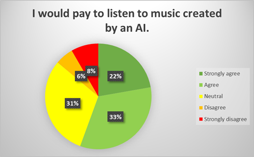
An interesting observation from the survey results is that around half of the people seem to be open to paying for music generated by an AI:

We have compiled the survey results in a bar chart that shows how the different features compare to each other when it comes to how much the subjects desired each of them. Knowing that for every feature the same number of subjects responded, this gives a good idea of the respective interests. Additionally, the graph shows the proportions of subjects responding mildly positive and very positive. This gives a better indication of the extent to which subjects were positive about these particular features.

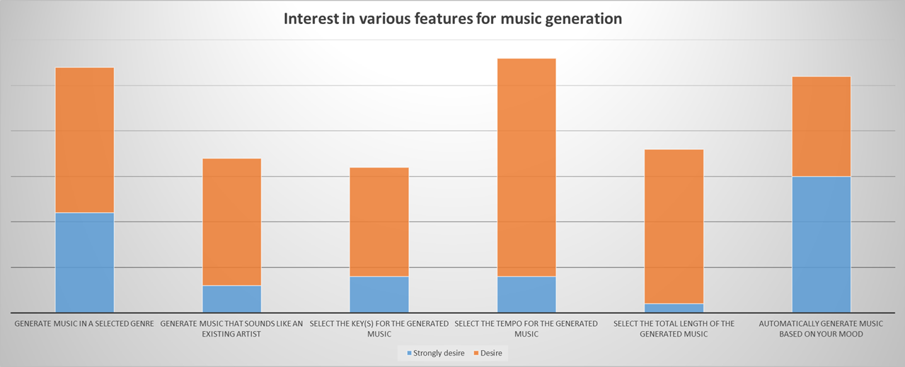
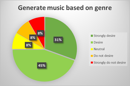
From these results we can see that in general user are definitely the most interested in generating music based on their selected genre, tempo and their mood. From these three, we can see that especially generating music based on mood seems to be very desirable, since many people strongly desire this feature. As for genre and tempo, we can see that they have a higher number of people interested in them in total, but a larger part of these people is only mildly interested. This is especially true for generating music based on tempo. To give an idea of the number of people interested in each feature, compared to people not interested, take a look at the following chart, that shows the distribution of people's desires for generating music based on genre.

Requirements

From the results of the survey together with our own ideas for the project, we have constructed a basic list of requirements for our product, which will be a website.

• The user shall be able to select a genre if desired.
• The user shall be able to select a tempo if desired.
• The user shall be able to choose a name for the generated song.
• The user shall be able to generate a song for any combination of genre and tempo.
• The user shall be able to generate a song without selecting a genre or tempo.
• The user shall be able to listen to the generated song.
• The user shall be able to download the generated song.
• The application shall give a brief explanation about how it works.
• The application should run on Google Chrome.
• The application should generate an audio file with synthesized sounds.
• The application should not generate a score.

Research (Alternatives)

Algorithmic composition

Besides using neural networks there are other methods to generate music. Two popular methods for music composition we looked at during our initial (literature) research are Mathematical models and Knowledge-based systems.

Mathematical models create music by encoding music theory with mathematical equations and using random events. These random events can be created with stochastic processes. This creates harmonically sounding, uniquely created music, respectively through its reliance on music theory, and the use of randomness.

Knowledge-based systems make use of a large database with pieces of music. The data is labeled, so that it knows what the characteristics of certain pieces are. It uses a set of rules to create “new” music, to match the characteristics given by a user. An example is a computer program called “Emily Howell”. It uses a database to create music and uses feedback from users, to create new music based on their taste.

None of these techniques generates sound on its own. It either creates a score or patches existing sound files together to create “new” music. We are curious of exploring methods that have not been used yet for the generation of music. Therefore we shall keep these techniques in mind, but cast our net wider so as to bring something innovative to the field of music generation.

Wavenet

To implement our Machine Learning idea to be able to mimic a certain artist we initially explored a Deep Learning algorithm called WaveNet. WaveNet is a deep neural network architecture created by Google Deepmind that takes raw audio as input. Already, it has been used successfully to train on certain dialects to create a state-of-the-art text-to-speech converter. Specifically, WaveNet has been shown to be capable of capturing a large variety of key speaker characteristics with equal fidelity. So instead of feeding it voice data, we intended to feed it musical input in order to train the network to generate our desired music. This has already been shown to work on piano music by the WaveNet team.

WaveNet was an attractive starting point for learning to work with neural nets because it is available as an open source project written in python using TensorFlow and is available on GitHub. This open source project was not created by the original DeepMind team, but it allowed us to easily train our first deep learning network using Tensorflow to get to know the technology and to ensure it is properly functioning on our hardware.

However, the results of WaveNet were not satisfactory, it was clearly not able to deal with the high level of heterogeneity of arbitrary music input. Furthermore, since this is already a proven technology made for a very specific goal, we thought it was less interesting to explore.

We trained WaveNet on the discography of David Bowie. An example of a sound file generated by the trained network can be found here.

Deep Learning

In this section, we provide an overview of the prerequisite knowledges of our work with respect to Deep Learning (and Machine Learning in general). Apart from the cited papers, it is noteworthy that we use the book Deep Learning by Goodfellow et al. both implicitly (e.g. for general models such as Artificial Neural Networks) and explicitly (e.g. for specific results) as a source throughout this section. Note that in the remaining sections we often use feature vector instead of metadata vector, this is in order to be consistent with terminology often used in literature.

Neural Network

Model of an Artificial Neural Network

Artificial Neural Networks (or simply Neural Networks) are large networks of simple building blocks (neurons or neural units) connected with many other neural units. A single neural unit is some summation function over its inputs, and can inhibit or excite connected neurons. Moreover, the signal produced by neurons are defined using an activation function, which generally sets a threshold value for producing a signal. Neural networks are inspired by the biological brain, although they are generally not designed to be realistic models of biological function . Instead, ANNs are so useful because they do not need to be programmed explicitly, instead they are self-learning. The challenges of designing an ANN include defining appropriate representations of the data, activation function(s), cost function, and a learning algorithm. Nevertheless, it is very useful for problems in which defining or formalizing the solution or relationships in the data is very difficult. Moreover, ANNs have the potential to solve problems we do not understand ourselves. For example, music is very complicated to formalize, especially without restricting to scores (i.e. sheet music), specific genres or limited varieties of music.

Model of an Deep Neural Network

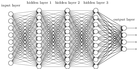
Using multiple neural networks as separate layers, one can construct a network with multiple hidden layers between the input and output layer: a Deep Neural Network. It is noteworthy that although Deep Neural Network are commonly used as an architecture in Deep Learning, it is not the only architecture used in the field of Deep Learning.

Generative Adversarial Networks (GANs)

A generative adversarial network (or GANs) is a generative modeling approach, introduced by Ian Goodfellow in 2014. The intuitive idea behind GANs is a game (theoretic) scenario in which the generator neural network competes against an discriminator network (the adversary). The generator is trained to produce samples from a particular data distribution of interest. Its adversary, the discriminator, attempts to accurately distinguish between “real” samples (i.e. from the training set) and samples generated/”fake” samples (i.e. produced by the generator). More concretely, for a given sample the discriminator produces a value, which indicates the probability that the given sample is a real training example - as opposed to a generated sample.

A simple analogy - to explain the general idea - is art forgery. The generator can be considered the forger, who tries to sell fake paintings to art collectors. The discriminator is the art specialist, which tries to establish the authenticity of given paintings, e.g. by comparing a new painting with known (authentic) paintings. Over time, both forgers and experts will learn new methods and become better at their respective tasks. The cat-and-mouse game that arises is the competition that drives a GAN.

More formally, the learning in GANs is a zero-sum game, in which the payoff of the generator is taken as the additive inverse (i.e. sign change) of the payoff of the discriminator. The goal of training is then to maximize the payoff of the generator, however, both players attempt to maximize its own payoff. In theory, GANs will not converge in general, which causes GANs to underfit. Nevertheless, recent research on GANs has led to many successes and progress on multiple problems. In particular, applying a divide-and-conquer technique to break up the generative process into multiple layers can be used to simplify learning. Mirza et al. introduced a conditional version of a generative adversarial network, which conditioned both the generator and discriminator on class label(s). This idea was used by Denton et al. to show that a cascade of conditional GANs can be used to generate higher resolution samples, by incrementally adding details to the sample. A recent example is the StackGAN architecture.

Generative adversarial networks have proven to be effective in practice, however, achieving stability is non-trivial. As such, we decided to build on top of an existing state-of-the-art architecture. Moreover, we attempt to follow good practice and successful strategies. For example, we normalize our input between -1 and 1, and use dense activation (e.g. Leaky ReLU).

StackGAN

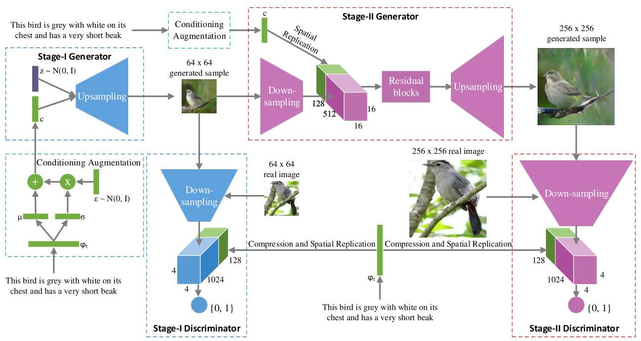
StackGAN uses two “stacked” generative adversarial networks to generate high-resolution (256x256) photorealistic images. This architecture utilizes two stages, corresponding to two separate GANs. The first network, stage I, generates relatively low-resolution images (64x64) conditioned on some textual description. This stage results in an image that clearly resembles the description, however, lacks vivid details and contains shape distortions. The second stage is conditioned on both the textual description and the low-resolution image (either generated by stage I; or for real images: downsampled). This results in convincing and detailed images of a higher quality than previously possible using a single level GAN.

Examples of bird and flower images generated based on text descriptions by StackGAN.

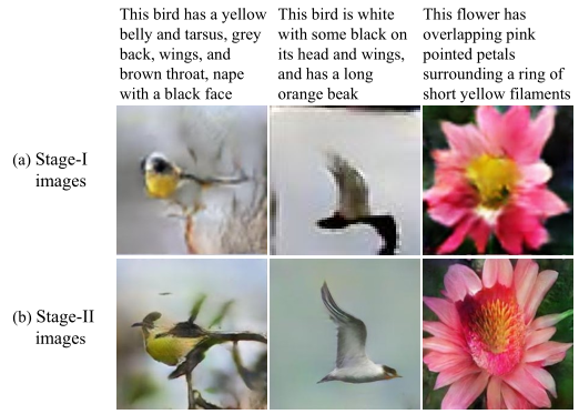
The actual networks are not conditioned on the text description itself, but instead of an encoded text embedding. Furthermore, in the StackGAN architecture more conditioning variables are added by sampling from a Gaussian distribution, with mean and standard deviation defined as a function of the text embeddings. This has multiple (mostly technical) advantages; including the ability to sample/generate multiple different images with the same textual description. This is also used to evaluate how varied the outputs are; two vastly different images can be generated using the same description.

We will discuss the StackGAN project and architecture in more detail when we present the work we did in adopting it to the MusicGAN, our attempt at a music generating GAN.

LSTM

An LSTM network is a recurrent neural network. Before the discovery of recurrent neural networks, it was not possible to use a network's previous experience to influence the task it is performing currently. For example, it was unclear how to use traditional neural networks to classify an event happening during a certain point in a movie, based on what had happened before in the movie. Recurrent neural networks address this shortcoming by passing in a previous output as an input parameter along with the actual input. Pictographically, this can be represented as a loop in a given piece of the network. The loop can also be represented as multiple copies of the same neural network, taking an old output as input for a new copy of the neural network.

It is these types of networks that have been able to produce very interesting results with speech recognition, language modeling, translation and music composition. More specifically, the LSTM---a specific type of recurrent neural network---has played an essential role in producing these results.

One of the main problems with regular recurrent neural network structures is the ability to use information that is essential for the context of the present task but occurred a long time ago. In other words, properly retrieving inputs from a distance that might be relevant for the present context is a difficulty.

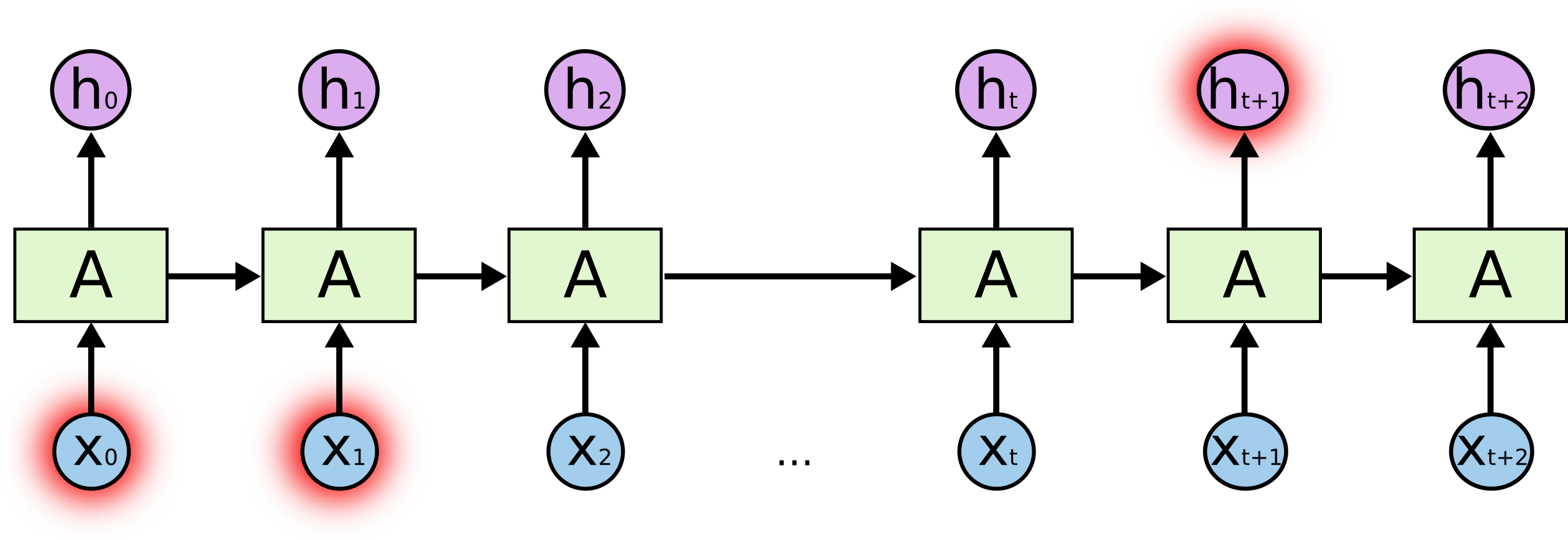
LSTMs were introduced by Hochreiter & Schmidhuber in 1997 and were explicitly created to deal with the long-term dependency issue. The main difference between a regular chain of recurrent neural network modules and an LSTM chain, is a cell state that holds and passes along information across the chain of LSTM network modules. Using this cell state, LSTMs can carefully decide what long term information to keep unchanged and what information to modify according to new inputs. These decisions are made using four neural network layers in each network module, unlike the one tanh layer in a typical RNN. The following diagrams depict the differences between a traditional RNN and an LSTM. Notice the persistent cell state towards the top and the 4 neural network layers in the LSTM.

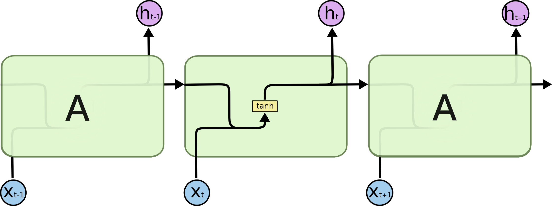
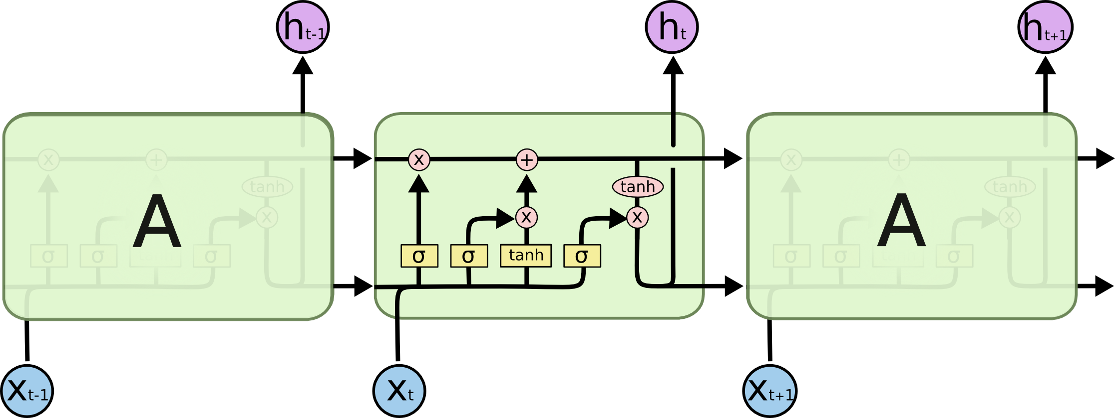
The first layer in the LSTM is responsible for deciding how much of each piece of information to keep in the cell state according to the output of the previous network module and the input to the current network module. The subsequent two layers decide what new information to add to the cell state. The last layer decides what the output of the current module is, using a filtered version of the current cell state that was modified by the previous three layers.

LSTMs have produced impressive results in a diverse set of fields. We were of course interested in its performance in music production. In 2002, Schmidhuber (one of the discoverers of LSTMs) along with some other researchers looked into finding temporal structure in music and found promising results. A very interesting part of the abstract: "Because recurrent neural networks (RNNs) can, in principle, learn the temporal structure of a signal, they are good candidates for such a task. Unfortunately, music composed by standard RNNs often lacks global coherence. The reason for this failure seems to be that RNNs cannot keep track of temporally distant events that indicate global music structure. Long short-term memory (LSTM) has succeeded in similar domains where other RNNs have failed, such as timing and counting and the learning of context sensitive languages. We show that LSTM is also a good mechanism for learning to compose music." Again, this clearly shows the advantage of being able to learn long-term dependencies, something that LSTMs excel at. Another paper in 2008 by Douglas Eck presents a music structure learner based on LSTMs. In their conclusion they note, "There is ample evidence that LSTM is good model for discovering and learning long-timescale dependencies in a time series. By providing LSTM with information about metrical structure in the form of time-delayed inputs, we have built a music structure learner able to use global music structure to learn a musical style.".

More recently, a Google brain project called Magenta has used LSTMs to create a bot that plays music with the user. In a later section we use their open-source framework to generate our own music samples.

Overview Components

Now that we have discussed what user needs we need to satisfy and have explored some technologies that might be suited for this goal, we can start looking into the components necessary to build the music generating application.

There are three major components necessary for constructing our product: the music generating Neural Network, the datasets from which to learn, and the user facing interface, for which we use a website.

In overview the product works like this: A user of the product inputs their preference on the website where upon the backend of the website forwards the request for a piece of music (based on the submitted preferences) to the Neural Network component. The Neural Network is tasked with generating music, but to do so it must learn what music sounds like, in particular how certain features (e.g. tempo) of music express themselves. The network learns from existing music, labeled with information such as the tempo, artist, instruments etc. Given a request for a piece of music the network will have to be trained on a dataset containing sufficiently many examples of music expressing at least some of the requested features. In the best case scenario the network can be pre-trained on a single dataset, such that every possible request can be serviced. A more realistic situation is that multiple instances of the network will have to be trained, each on a separate dataset, such that one of the instances corresponds well to certain types of feature requests. Assuming that the Neural Network has been appropriately trained, the generating of the new piece of music is a straightforward process of feeding in the encoded features to the inputs of the network, propagating the inputs throughout the network, and finally converting the network outputs to a proper audio file. This output audio file becomes available in the user interface as the result for the user.

We will now discuss our choices regarding the datasets, the Neural Network setups that we deemed fitting, in GAN form, but in LSTM form as well, and finally we take a look at our user facing component.

Datasets

When looking for datasets to train the Neural Network on, we encountered 3 main sources: The One Million Song dataset, the Free Music Archive (FMA) data set and the MusicNet set. Each of these will be explained in detail in the sections below.

Million Song Dataset

The Million Song Dataset was the first dataset we found when looking for large free music datasets online.The Million Song Dataset is a collection of audio features and metadata for a million contemporary songs (donated by Echo Nest) and hosted by Columbia University (NYC) to encourage the research on algorithms that work on large datasets. It was by far the biggest dataset we found (around 300gb of musical metadata for over a million songs), but unfortunately also one of the oldest and and most difficult of all: it actually contained no audio files in the dataset. According to the Million Song website, this wasn’t suppose to be a problem since they had scripts to easily scrape songs off of the 7digital site (a website similar to iTunes) using the 7digital API. But, the Million Songs’ pythons scripts were over 7 years old (with no maintenance done) and required old python libraries riddled with inconsistencies. After several failed attempts to get it working, we were forced to start from scratch in building our own script to extract songs. This underestimation of the difficulty of actually getting the audio files proved to be the biggest obstacle with this dataset. So in summary, this combination of old documentation, the sheer scale of the amount of data and inconvenience of not having the song files readily available made this one of the hardest datasets to work with.

Free Music Archive

The next data set is the “Free Music Archive” (FMA) which we found after we realized how difficult the One Million Song set would be. The Free Music Archive (FMA) dataset was created by researchers at the École polytechnique fédérale de Lausanne (EPFL) with the intention of helping push forward machine learning on music. Even though this dataset was much smaller than the One Million Song set, it importantly contained the actual audio files (in mp3 format) within the set. Being that this set was only released recently (December 2016) only the small and medium versions of the set were available (sizes of 4,000 and 14,000 songs respectively) with the large and full size sets to be released sometime later. Conveniently, the metadata and features were stored in a JSON file, allowing for easy access using a Python library called pandas. This meant that all had to be done was write a script to format the data into a form that the neural network would accept (described in a later section). Furthermore, data in the metadata files included things like song ID, title, artist, genre and play counts. Additional, the audio provided was taken from center sections of the songs since the middle of songs was considered to be the most active/interesting by the researches providing the media. However, when going through some of the song clips, it was found that the quality wasn’t as high quality as expected (some recordings sounded as if they were live performances) and each genre wasn't as homogeneous as expected.

MusicNet

The last dataset we considered was the MusicNet set which was the smallest (330 songs) but the most homogenous (all classical music) and had the most comprehensive labeling of any of the previous sets. Note here that these are 330 full songs of about 6 minutes each, so comparably it is still a significant data set. This set included over 1 million labels with features such as the precise time of each note, the instrumenting playing each note, each note’s position in the structure of composition. Due to the superior labeling, this was the dataset we ended up training our neural network on.

Initial investigation showed that while the dataset had 11 instruments, by far the largest portion of music only contained 4 instruments, and for the other 7 instruments there was very little data. Therefore, we decided to only select songs with these 4 instruments. We generated samples in the following matter. We cut each song into samples of 4 seconds each. For each sample we checked if at least 4 notes are played within this sample, otherwise we reject the sample. This is to ensure that we do not have samples which are silent.

We generated a feature vector for each sample in the following matter. We encoded data like which composer and composition was playing and the ensemble type using one-hot encoding. We then cut the sample into 16 pieces of equal length (thus each piece is 0.25 seconds). For each piece we encoded which instrument had an active note again using one-hot encoding. This to provide as much labeling to our neural net as possible, to increase the chance of success.

Representation

The scripts that extract data from the datasets create two vectors. One vector contains the information about the song (the raw song data) and the other vector contains the metadata. The vector containing the song data is created with the help of the Librosa library. The library loads an audio file as a floating point time series. The length of the song vector is the duration of the song multiplied with the sample rate. The vector containing the metadata is created with the help of the pandas library. The metadata of the datasets are extracted from a JSON file in the case of the FMA dataset or from a CSV file in the case of the MusicNet dataset. The feature vector contains categorical data and floating point data. Each category of categorical data is stored as separate entries in the vector with the value 1 in the entry, when the song belongs to the specified category or value 0 otherwise. For example, in the feature vector for the FMA dataset, each genre is encoded with a separate entry in the feature vector. If the song belongs to a certain genre, then that entry in the feature vector is 1, otherwise that entry will be 0. The reason for this approach is to prevent the neural net from learning a linear relationship between the genres as such a relationship does not exist. You cannot say that rock is two times blues. The floating point data has exactly one entry in the feature vector. The entry contains the value of that data. For example, for the tempo entry, the entry will contain the value of the beats per minute of the song. This type of data does contain a linear relationship. You can say that 200 beats per minute is twice as fast as 100 beats per minute.

MusicGAN

In this section we describe our work on MusicGAN. MusicGAN uses the implementation and architecture of StackGAN as a base. Three vastly different approaches are implemented, executed and evaluated (iteratively when problems/challenges were found). We first describe in detail how StackGAN works, why we use it, and what limitations it poses. We then describe the three different approaches and the underlying theory. Finally, we present the results of the three approaches.

StackGAN

The StackGAN architecture uses two “stacked” generative adversarial networks to generate high-resolution (256x256) photorealistic images based on a textual description. The stacked nature of the architecture refers to using two GAN setups conditioned on text input, named Stage I and Stage II. These two networks correspond to phases in the learning process. The architecture needs a sufficient amount of properly labeled data (i.e. correct text description for real images of birds/flowers/etc.) to learn from.

The Stage I phase is concerned with learning how to produce low resolution (64x64 RGB pixel) images that are somewhat convincing for a given text description. Given the results of Stage I, the Stage II network takes the low resolution image produced for a text description by the Stage I network, adds the text description again, and takes these two as the input to the generating process. The output of Stage II are high resolution images (256x256 RGB pixels). The idea is that the second stage will be able to add details to the image, or even correct “mistakes” from the low resolution generated image, such that the final result is truly a convincing image given the text description. This method of stacking GAN networks was very successful applied by Zhang, Han, et al. to generate convincing images of birds, see figure. In the same paper this method was equally successful in generating images for flowers from text descriptions.

Example of quality of bird images generated by StackGAN.

Stage I

First the generator and discriminator networks of Stage I are trained. The generator network learns how to produce low resolution images, still only containing basic shapes and blurs of colors, that are convincing to the discriminator network, which gets incrementally better at detecting forgeries, while at the same time the generator becomes better at creating these fake low resolution images.

The output of the generator is in the form of 64x64 RGB images, represented as 64x63x3 tensors (a tensor can be thought of a multidimensional array, and can also be used as a mapping between multidimensional arrays), where the last dimension has three indices, due to the red, green and blue channels of the image. The input neurons of the generator are an encoding of the text description, a topic we will not touch on, together with a noise vector, which, when adjusted for one text description, makes the image generation nondeterministic. A series of upsampling blocks (deconvolution) layers are applied, each time producing a 3x3 block of neurons for each neuron in the previous layer. After a number of layers the required output size is reached. The tanh activation function is used as a final activation to make sure that the output RGB channels values are constrained to [-1,1]. The discriminator network works by taking an input image as a 64x63x3 tensor, along with the text encoding, and apply convolution layers (going from a square of 4x4 down to a 2x2 square) to go eventually to a single neuron whose activation is used to determine whether the discriminator believed the input to be fake or real. For every (de-)convolution layer ReLU activations functions are applied. A feature of the actual architecture that we will not discuss in detail is that the networks actually work by batching, which means that 64 images are generated/fed into the networks at the same time. This does not have significant consequences for the above description, as the most important change is that tensors gain an additional dimension with 64 indices for the separate inputs/outputs. For more details we refer to the StackGAN paper.

The training process occurs by feeding the discriminator with a combination of real and fake images. The weights of the network are adjusted by backpropagation according to whether the discriminator was successful in identifying the realness of the input. Among the fake inputs are mismatched text descriptions and real images, but also, of course, the images generated by the generator network. The generator’s success is measured by whether it was able to fool the discriminator network. Initially both the discriminator and the generator know nothing, but iteratively they are able to improve due to improvements made by their opponent.

The StackGAN architecture.

Stage II

The Stage II generator network takes a text encoding along with a 64x64x3 tensor encoding of an image as input. By applying upsampling blocks the networks expands the input to a 256x256x3 output layer, which represents the final image. The discriminator for Stage II is largely the same as the Stage I discriminator except now it has even more downsampling layers.

The training for the discriminator is similar to Stage I, its network weights get adjusted based on whether it is able to detect fake images from real images. The generator now works a bit differently, namely that a text description will first be fed to the trained Stage I generator. The output from Stage I is then fed into the input of Stage II along with the same text description. Based on this input the generator produces its high resolution output. As an additional scenario for generating fake images the generator is fed downscaled real images with the corresponding text description.

From StackGAN to MusicGAN

Of the technologies that we encountered during our research phase we were especially impressed by the successes that were being attained by Generative Adversarial Networks. In the search for an appropriate technique for generating music we were encouraged to opt for GANs by the following quote from an answer on Quora, by Ian Goodfellow, inventor of the GAN architecture: “In theory, GANs should be useful for generating music or speech. In practice, someone needs to run the experiment and see how well they can get the model to work.” Using the GAN approach to generating music is also an attractive proposition due to the networks learning by example from a dataset, and does not require a deep and profound theoretical understanding of what makes an image look like a bird, or a piano song sound like a piano song. Also the advantage of the approach of directly generating generating audio samples versus scores or the like is that we could capture the complexity of multiple instruments playing together, a common feature of music. This is in opposition to existing score generating approaches (for a single instrument) such as the Magenta project discussed in a later section.

The StackGAN architecture is one of the most impressive recent GAN approaches. The following features of StackGAN were particularly attractive for this project:

• The resolution and level of detail that StackGAN is able to achieve. In particular important for the length of the music fragments we want to produce.
• The publicly available source code, developed in one of the major Deep Learning libraries, TensorFlow , such that we can be build upon a proven product and enjoy the benefit of an active community.
• The training sessions remain basically unchanged. It is possible to change out the data sets and only modify the code so as to deal with the change in data representation.
• The goal of generating images. When we consider Fourier Transforms we also get a two dimensional representation, which means that for one modification approach we only need to do minimal work on the code.

There are also some limitations to the chosen (Stack)GAN method:

• The StackGAN project’s goal of producing images assumes that a two dimensional structure for the data is appropriate. While this might be obvious in the case of images, in the case of audio it might not be the best choice to have have this representation assumption embedded in your network structure.
• While being able to work with the entirety of the codebase for the StackGAN project is definitely a plus in terms of being able to “stand on the shoulders of giants”, the complexity of the entire project is considerable.
• The resolution for the images is not that high when compared to the number of samples that normally are present in an average length song, i.e. in an average song is about 240 seconds (4 minutes) in length, at a cd-quality sampling rate of 44.1kHz that would mean that you would need to generate 240*44,100=10,584,000 separate data points for a complete song, while the StackGAN architecture was only able to generate 256*256*3=196608 separate data points. Due to viability concerns with trying to scale up the architecture we will restrict our music fragment length to 4 seconds, with for Stage I only low frequencies up to 1 kHz, and for Stage II frequencies up to 16 kHz.

Before we look at the separate approaches we took in modifying the StackGAN project into a music generating MusicGAN, we need to mention that instead of the text encoding that was fed into the networks as a description of the image, we use the metadata vector obtained from the datasets as a description of the audio that is input.

Approach: Representation Learning

Example of different representation (by David Warde-Farley)

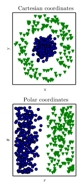
Many tasks can be either very easy or very difficult, depending on how the problem is represented. For example, imagine that we have two different representations of the same dataset. The task at hand is to draw a straight line that divides the two kinds of data points (indicated by colour and shape) as well as possible. Clearly, using polar coordinates as a representation of the same dataset makes the task at hand much easier. However, for real problems in machine learning, finding an appropriate representation (i.e. one that makes learning easier) is non-trivial and has several serious disadvantages. In particular, finding a good representation by hand is often a very lengthy process, on which researchers spend multiple months or even years. A different approach is Representation Learning (or Feature Learning), which are techniques used to learn an appropriate representation (automatically). This approach was inspired by Goodfellow, who states that learned representations are often effective in practise.

Learned representations often result in much better performance than can be obtained with hand-designed representations.
—I. Goodfellow et al., Deep Learning (2016)

In our case, we feed the network data in the .wav or WAVE (Waveform Audio) File Format. However, it is noteworthy that raw music data files in different formats should work without much work. The idea is that the network learns to transform this data into some representation with the shape of a square RGB-image (due to the architecture of StackGAN). Intuitively, we like to think of this representation as a 3-dimensional spectrogram.

By slightly extending both the generative and discriminative networks with an additional (de)convolutional layer, we transform the data from raw music to the dimensions of the images used in StackGAN. As such, the architecture of StackGAN remains almost unchanged. More specifically, in Stage 1 the music is transformed to a 64x64x3 tensor (64x64 RGB image), and in Stage 2 to a 256x256x3 tensor. For example, the stage 1 generative network outputs a 64x64x3 tensor. We add a final (deconvolutional) layer to the network which converts the image back to the dimensions of the original music. Furthermore, we change the original last layer to use a leaky ReLU activation function, instead of the tanh originally used. We do this because only the last layer should use the tanh activation function. In this added layer, we experimented with multiple kernel and stride dimensions, as long as they resulted in the dimensions of the original music. Finally, we reshape to ensure that the shape of the output is a vector of 1xn, where n is the number of samples in the music file. For the discriminative network, an initial layer is added. Note that the discriminative network is now given data in the format of the music samples (both the real samples and the adapted generator’s output). As such, we have a convolutional layer that changes the input to the dimensions of the original network (64x64x3 in stage 1). The layer uses Leaky ReLU for activation, as do other layers (except for the last) in the StackGAN’s layers.

Note that even with above description there are multiple choices we can make. In particular, how the samples are taken is important. One choice to make is related to the size of the samples. For example, if we give the Stage I network a fragment with more sample points than 64x64x3, then the layers we added are forced to compress and decompress the music. An advantage is that we can use the fragments for both the stage I and stage II networks. Furthermore, the network can “decide” which information to store and which to get rid of (i.e. unimportant on the output). A large downside is that real fragments will not be compressed (and decompressed), which potentially makes it easier for discriminator to beat the generator. As such, we choose to simply sample samples at a sample rate such that a single sample has 64x64x3 sample points. Since we are evaluating whether this approach works, we decided to simply set a very low sample rate for the Stage I network. This is not very convenient when training Stage II, since we essentially provide the same samples to stage 2 except including more mid-high range sounds. However, since we are trying to establish whether this approach could work, this strategy works best as it allows us to evaluate the progress of the stage 1 network. In other words, if this strategy does not yield progress after training stage 1, it is senseless to train stage 2. Finally, note that selecting larger samples than 64x64x3 (thus requiring compression), essentially results in the added layers functioning as an autoencoder.

Intermezzo: Short Time Fourier Transforms

As an alternative to having the network learn the representation itself for the following two approaches we now consider picking a representation.

That any particular sound wave is composed of many interfering waves at distinct frequencies is a basic law of physics. Fourier Transformations are a way of decomposing a sound wave into the different frequencies, e.g. decomposing a chord into its constituent notes. The result of applying a Fourier Transform to an audio fragment is that you obtain a list of complex numbers, one for each frequency, such that the magnitude of the complex number of that frequency represents the amplitude of frequency within the audio fragment and the angle of the complex number represents the phase of the frequency. The Fourier inversion theorem says that given that we know all the frequency and phase information of a wave we can reconstruct the wave, meaning that we can obtain back our original sound fragment from our decomposition information. One result for Fourier Transforms is that one needs to analyse at least half the number of audio samples of frequencies to analyse for the inversion to be accurate. Note that the amount of degrees of freedom for an audio sample and the amplitudes for each frequency is the same, since the amplitude consists of a real and imaginary part while the audio sample only consists of real numbers.

An important technique for the analysis of music is to not take the Fourier Transform of the entire music fragment but to split up the music fragment into many short fragments and applying the Fourier Transform to each of these short fragments. This technique is called the Short Time Fourier Transform (STFT). What is gained from this type of analysis is that one can see the progression of the presence of certain tones throughout the entire music fragment by looking at the presence of frequencies in each short time window.

Example of spectrogram for an audio fragment of human speech

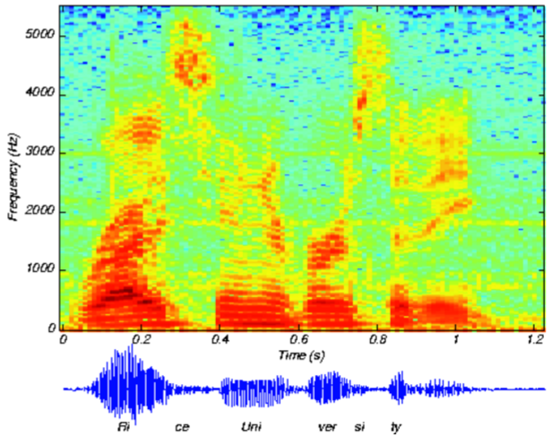
The accompanying figure is called a spectrogram. A spectrogram is a plot of the amplitude for the presence of frequencies in short time window for an audio file, in this case a speech audio fragment. The vertical axis are the frequencies, the horizontal axis is the time, and the color dimension represents the amplitude for each frequency at the short time slice in the audio file. (Note that the phase information from the STFT is ignored.)

Note that the splitting up of an audio file into many time windows and where for each of these time windows the strength of the presence of many frequencies is recorded gives a representation of audio that is much closer to the two dimensional representation of images.

We used the librosa library to convert between audio wave representation and Short Time Fourier Transform representation (STFT). We chose the parameters of the STFT in such a way to match the size of the image input we required, e.g. for stage 1 we often wanted 64 horizontal points so we chose the sample rate accordingly. The window size was in general determined by the vertical dimension required by the network. In all cases we chose a hop length of half the window size.

Approach: Complex Images (STFT)

The second approach of encoding music as images uses the Short Time Fourier Transform discussed in the previous section. With these technique, we can generate a 2D matrix representation of the music sample. However the entries are complex numbers which is poorly supported in TensorFlow (technically complex valued neural networks are possible). Our initial goal is to represent these as regular 64 by 64 images with 3 channels so that we do not have to alter the architecture (since time was of the essence and this is the original input format of the StackGAN architecture).

To achieve this, we preprocessed the samples as follows. First we played with the parameters of short time fourier transform and the sample rate such that we generated a 64 by 96 amplitude matrix M. For each row of the matrix, we then split the complex numbers into its real and imaginary parts resulting in matrix M’. Let M(i) denote row i of matrix M. Then M’ is defined by M’(2i) = Real(M(i)) and M’(2i+1) = Imaginary(M(i)). This resulted in a 64 by 192 matrix M’. The next step was then to put the first 64 rows of M’ in channel 0 of tensor T, the next 64 rows in channel 1 of tensor T, and the next 64 rows in channel 2, such that T is a 64x64x3 tensor. This tensor was finally normalized such that values ranged from -1 to 1 (since the deep learning network can only output values between -1 and 1, because the last layer has a tanh activation function). The result was fed to StackGAN as the input for the first stage.

Approach: 2-D Spectrograms (STFT)

For this final approach we turn again to the Short Time Fourier Transform, but use the most straightforward mapping to the main idea behind the StackGAN network, namely that pixels get upsampled and downsampled.

For this approach we take the view of the STFT as being a two dimensional representation, with a time (window) dimension and a frequency dimension, where both of these dimension are discrete. At each discrete index in this representation we have a complex number representing the amplitude and phase which corresponds to the strength of the presence of the frequency at that time slice. As the complex number has the natural “2D” representation of amplitude and phase, one can view this as two channels of a pixel (where the spectrogram only used the amplitude as one channel for a pixel).

As such we modified the network to no longer take 64x64x3 tensors (for RGB images with 3 channels per pixel) but instead to take 64x64x2 tensors.

Results

Approach: Representation Learning

For this approach we altered the architecture of the network such that it has direct music as input and directly outputs music. We did this by adding one additional layer at the start of the discriminator network, and one layer at the end of the generator layer. The responsibility of this layer was to encode the music to and from a 64 by 64 by 3 image. Note that the input of the first stage of StackGAN had quite low frequencies. This is an example of an original music file:

https://soundcloud.com/noud-de-kroon/target-representation

Initially the neural network only output static. An example output is this:

https://soundcloud.com/noud-de-kroon/initial-representation

After 75 epochs (an epoch is a cycle in which all the training data is trained on once) the output was as follows:

https://soundcloud.com/noud-de-kroon/epoch75-representation

Possibly there might be some rhythm being learned by the network at this point (but this might also be caused by some unknown factor. After this unfortunately, the training quickly falls into a failure mode. The discriminator loss quickly approaches 0, which implies that the generator is never able to fool the discriminator, which causes process to halt. This is a known problem that may be encountered when training GAN’s (as mentioned for example here. At epoch 300 the output of the network is as follows:

https://soundcloud.com/noud-de-kroon/final-representation

At this point training was halted since it seems a lost cause.

Approach: Complex images (STFT)

This approach was the first architecture we were able to implement and run (apart from the original StackGAN architecture on images). The first trial was unsuccessful, and the resulting output did not improve while training. The initial output was as “close” to the groundtruth (and, by extension, to “random noise”) as the final output (after 600 epochs of training) was. The discriminator very rapidly took over (having a loss very close to 0), and the generator was unable to “learn”. We inspected the results, and noticed that the generated music was in a very small range, whereas the real music had a much larger range. We realized that the mistake we made was that the generated output has values in (-1, 1) by design (tanh activation function). However, the real data samples were not normalized appropriately (as normalization of images is vastly different). Furthermore, when storing the output, we should denormalize the generated music. In short, we normalize the (real) samples using the maximum and minimum value of all samples. Finally, we denormalize the generated samples using these same max and min values. With these modifications, the results were still not very successful unfortunately. Although there seemed to be small improvements, we were not convinced that the network was learning sufficiently regarding the internal structure of the music data. As such, we did not continue with stage 2.

Approach: 2-D Spectrograms (STFT)

For this approach we had to somewhat alter the inner structure of stackGAN. This to make it handle 64 by 64 by 2 tensors (instead of 64 by 64 by 3). While this was a relatively minor adjustment, it required understanding the internal structure of stackGAN to make the proper adjustments. Sound was sampled at 1 kHz. An example of a sound sample is given here:

https://soundcloud.com/noud-de-kroon/target-approach-3

An example of initial network output is given here:

https://soundcloud.com/noud-de-kroon/epoch-0-approach-3

After 75 epochs the output sounded as follows:

https://soundcloud.com/noud-de-kroon/epoch75-approach-3

After 300 epochs the output sounded as follows:

https://soundcloud.com/noud-de-kroon/epoch-300-approach-3

And finally when training completed at 600 epochs the output sounded as follows:

https://soundcloud.com/noud-de-kroon/epoch-600-approach-3

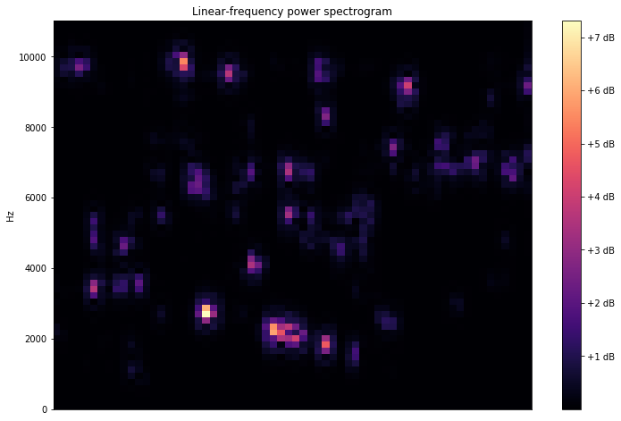
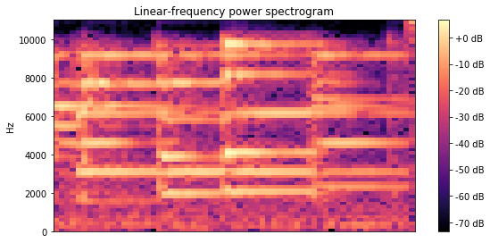
Looking at the spectrograms, a generated sound file looks as follows:

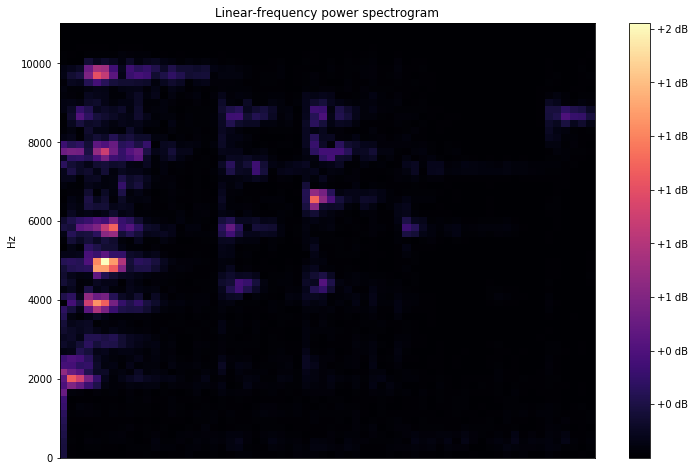
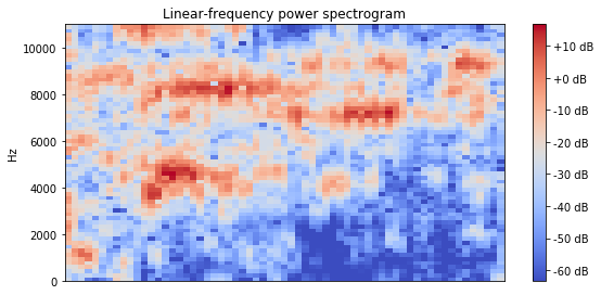
While a fake sample looks as follows:

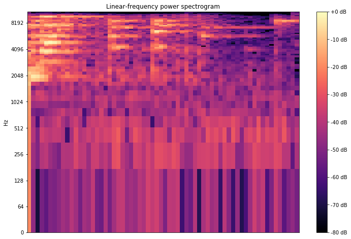
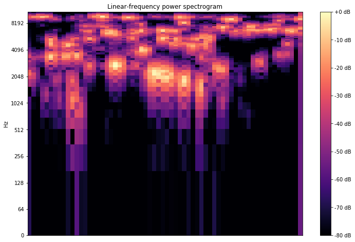
Looking at the spectrograms it definitely seems the network has learned to represent the magnitude quite well. However, at this point we realized that we used a linear scale for the amplitude, while human hearing generally works on a logarithmic scale. If we compare the spectrograms on a logarithmic scale we yield the following results for the real sample:

And the following for the generated “fake” sample:

Here we can clearly see that there is still a big difference between the samples. As a result, we decide to again train the network, but now first log-transform the amplitudes before scaling it to -1 to 1. The following is again then a real sample (using logaritmic scale):

And the following is a fake sound fragment:

Challenges

This was one of the most technically challenging projects we have encountered so far during our bachelors. In this section we would like to discuss some of the problems we encountered while adapting stackGAN.

Firstly, the original source code has a very high degree of complexity and is poorly documented. StackGAN relies on the TensorFlow library, which is a very high level library. This means that a single function call can be quite hard to understand, and might have many side effects. This made effectively working together on the code very hard, since any change to the code should be very well thought through and required understanding of the entire project. Another difficulty related to this is that starting the software project took around 5 minutes. This meant that if there was a bug somewhere, we would have to try fix the problem, start the project, wait 5 minutes, check the result, and then start the process over again. This made working on the project very cumbersome.

The second challenge was that hardware intensity of training deep neural networks. We had two computers with hardware sufficient for training deep neural networks. During the final 2 weeks of the project, these computers were training 24/7. If we tried a new strategy, we would only see results a few days later. This made iteration very slow.

The first two challenges combined caused us not to experiment with running a stage 2 of the network, especially because stage 2 is even more hardware intensive than stage 1. The MusicNet dataset for stage 2 is around 40 GB, and training stage 2 would take approximately 5-7 days. Running stage 2 would only be beneficial if stage 1 actually provided good results, thus we thought it was more important to improve the result of stage 1 and we could iterate more often on stage 1. In the end we believe stage 1 still does not provide good enough output for stage 2 to have potential to generate good output.

We also attempted to use Amazon Web Servers and Google Cloud. Unfortunately, we needed a server with GPU. Both Amazon and Google requires extra administrative work to be allowed to use instances with GPU’s. Unfortunately, we were not able to get these approved in time.

Finally, note that in the results we do not analyze how the network responds to different feature vectors. This is because the results we obtained are not clear enough to hear or see the difference between instruments or styles present in the music. We therefore feel that at this point, with the current quality we manage to obtain, analyzing how the network reacts to different feature vectors is not fruitful.

Experimental LSTM

One of the biggest problems with relying on GANs throughout the entire project is that they have never before been used to create music. We could not be certain that the output of that network would be successful. Therefore, as a backup plan, we researched a different type of network called the Long short-term memory (LSTM) network, which has already produced good quality results. One of the main difference between GANs and LSTMs---also what makes GANs more impressive---is the way they take input. Our approach with GANs relies on inputting raw audio while our LSTM approach relies on ultimately taking text input.

Magenta

"Magenta is a Google Brain project to ask and answer the questions, “Can we use machine learning to create compelling art and music? If so, how? If not, why not?” Our work is done in TensorFlow, and we regularly release our models and tools in open source. These are accompanied by demos, tutorial blog postings and technical papers. To follow our progress, watch our GitHub and join our discussion group. Magenta encompasses two goals. It’s first a research project to advance the state-of-the art in music, video, image and text generation. So much has been done with machine learning to understand content—for example speech recognition and translation; in this project we explore content generation and creativity. Second, Magenta is building a community of artists, coders, and machine learning researchers. To facilitate that, the core Magenta team is building open-source infrastructure around TensorFlow for making art and music. This already includes tools for working with data formats like MIDI, and is expanding to platforms that help artists connect with machine learning models." We used the LSTM models released in the open source Magenta project to experiment with this approach to music generation.

Data

We used MIDI files for the LSTM network. The data sets we planned on using was the Lakh MIDI Data set and a data set created by a redditor called The MIDI Man . The data set created by The MIFI Man contains information about the artist and the genre of the MIDI files. The Lakh MIDI Data set consist of several versions. The version we are used is the LMD-matched version. This version is a subset of the full version of the data set. This subset had all its MIDI files matched with the metadata from the one million song database.

LSTM Model Configuration

The magenta framework allowed for three types of LSTM configurations which our results were based on.

Basic

This configuration acted as a baseline for melody generation with an LSTM model. It used basic one-hot encoding to represent extracted melodies as input to the LSTM.

Lookback

The lookback RNN introduced custom inputs and labels. The custom inputs allowed the model to more easily recognize patterns that occur across 1 and 2 bars. They also helped the model recognize patterns related to an event's position within the measure. The custom labels reduce the amount of information that the RNN’s cell state has to remember by allowing the model to more easily repeat events from 1 and 2 bars ago. This resulted in melodies that wander less and have a more musical structure.

Attention

In this configuration we introduced the use of attention. Attention allowed the model to more easily access past information without having to store that information in the RNN cell's state. This allowed the model to more easily learn longer term dependencies, and resulted in melodies having longer arching themes.

Results

We were able to produce some preliminary results using Magenta's pre-trained models. It is interesting to hear the differences between the various configurations (basic, lookback and attention) of the LSTM.

Basic Recurrent Neural Network Example 1

Basic Recurrent Neural Network Example 2

Lookback Recurrent Neural Network Example 1

Lookback Recurrent Neural Network Example 2

Attention Recurrent Neural Network Example 1

Attention Recurrent Neural Network Example 2

The next two samples were generated by priming the LSTM with the first four notes of "Twinkle Twinkle Little Star" using the attention recurrent neural network.

Twinkle Twinkle Little Star Example 1

Twinkle Twinkle Little Star Example 2

User Interface

With our target user type being an average music listener, we needed a simple interface that hides the technical details from the user. The small number of features, that we based on the survey results, reduces the freedom users have in customizing their music, but in turn greatly simplifies the use of the application. By doing this the user does not get overwhelmed by features for something that is already a new technology anyway. It must also be stressed that the current level of our music generation network is not high enough to provide a wide range of customizable input either. Therefore, this application is only the first step in providing this technology to the user, and by no means a finished music generation tool. The current version of the application only has the most important features, that we found in our survey.

Website

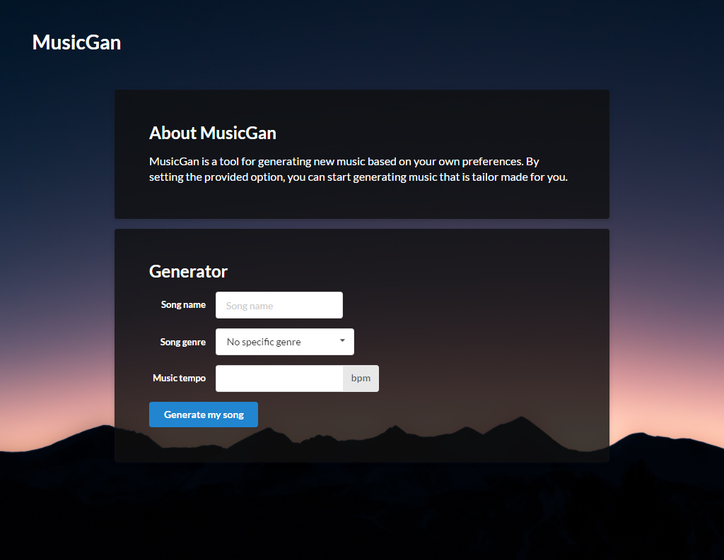
To create the interface described above we used a basic setup with Laravel as the backend framework and Semantic UI as the style framework. The interface we created is shown in the figure below.

The most recent version of the live website is available at MusicGan.eu.

User Feedback

To make sure our product actually satisfies potential users, we need to evaluate it by having them try it out and ask them questions. By doing this we want to find out the following things:

• Is it clear for the user what the application is doing?
• Is it clear for the user how to use the application?
• Is the user satisfied with the available options?
  • If not, what options are missing?
• What does the user think of the generated song?
  • Does it reflect the selected options?

By asking people around us (friends and family), we found that our application could be improved in a few ways:

• Problem: It is hard for the average user to equate a certain number of beats per minute to an actual speed.
  • Solution: Change the tempo selection to a slider or multiple choice option, where the user can choose between a range from slow to fast, while not being aware of exact numbers.
• Problem: Not all genres that users want are available.
  • Unfortunately we will always be limited by the genres in the dataset when we generate music based on a genre.
• Problem: The limited options make the application seem somewhat useless, since one might as well search for existing music with the right filters.
  • Solution: Since this technology is still new we are very limited in the options we have, and therefore the user’s choice is also limited. As the technology develops further, the user shall be able to give a better specification of what they want. As we saw in the survey, users seem to be interested in generating music based on emotion. This is one example of how music generation might become more advanced in the future, and so become more valuable to users too.

Next to this critical feedback we mainly noticed that, because of its simplicity, users did not seem to have problems user the application. Since the quality of songs we have been able to generate so far have not been good enough to present to the users, we did not receive feedback on those. Overall, users seemed very curious about the possibilities and wished to have more control over the generation process. Of course, the main reason why we have been unable to deliver that is that the current level of our generation software does not allow for that flexibility yet. Furthermore, we have put our focus on generating any music at all, since this problem was already hard enough to begin with.

Discussion

GAN

While the results were far from perfect, there seems to be some promise for using GAN’s to generate music directly. Looking at the output of the approach using 2-D spectrograms, there seems some potential in this approach, however especially the sensitive nature of sound seems to be an issue (because of the logarithmic nature of human hearing). Further research is required to keep improving on this result (which is something a few of us plan to do during the summer holidays).

One thing to note is that StackGAN is from the ground up built to process images. While using StackGAN allowed us to get results within the short time span allotted to this project, we feel that in order to properly attack this problem, from the ground up music has to be kept in mind. This mostly shows itself in the fact that kernel sizes of convolutional layers of the layer are chosen such that features of images can be recognized. We need to rethink these kernel properties in order for the layers to be able to detect features relevant to music.

LSTM

It would have been interesting to explore the extent to which we could have molded Magenta's LSTM technology to the needs of our users. As is described in the Experimental LSTM section, we achieved output of pre-trained models and found datasets to use. We did not pursue further because we decided that we did not want to dedicate many of our resources towards the backup option while the GAN approach still showed promise. The idea was that if all GAN approaches showed unimpressive results, we would shift our focus to existing technologies like LSTMs, and the limited resource (usually one person) would be able to quickly bring everyone up to speed on the backup approach. If this did happen, we would first work on training our own LSTM and tweak it towards what we found our users are looking for, like generating samples based on genre, existing artists and tempo. We were happy that we were not forced to follow this path; we were much more interested in discovering new ways of generating artificial music rather than using existing technologies. Nevertheless, it would have been a valid approach for the product we were trying to build for our users, and might have even produced better results.

UI

In general people were quite receptive to our ideas and our UI. Improvements from the user’s perspective are that users want more control, since only genre and tempo are very limited. Ideally we would find an intuitive way that would allow the user to control the generation process to create music that perfectly suits their needs.

Final Thoughts

Throughout this project we have learned a lot and we are satisfied with our results. The research we have done has shown that there is quite possibly a legitimate market interest for artificially generated music. The results we have gotten from exploring different methods of generating music have surprised us in a positive way and show that this interest might be satisfiable in the near future, should these techniques be developed further. Therefore, we definitely feel that it is worth pursuing this project further. And finally, we learned a lot about dealing with uncertainty and morale in a R&D focussed project. Especially this last part was challenging, since at many points it was hard to keep believing that the final results would be worth all the effort. Reflecting back on the project, we think we chose a very difficult subject, but it was the topic we were most interested in exploring and in the end we managed to make it work for us.

Planning

Gantt chart

The Gantt chart of this project

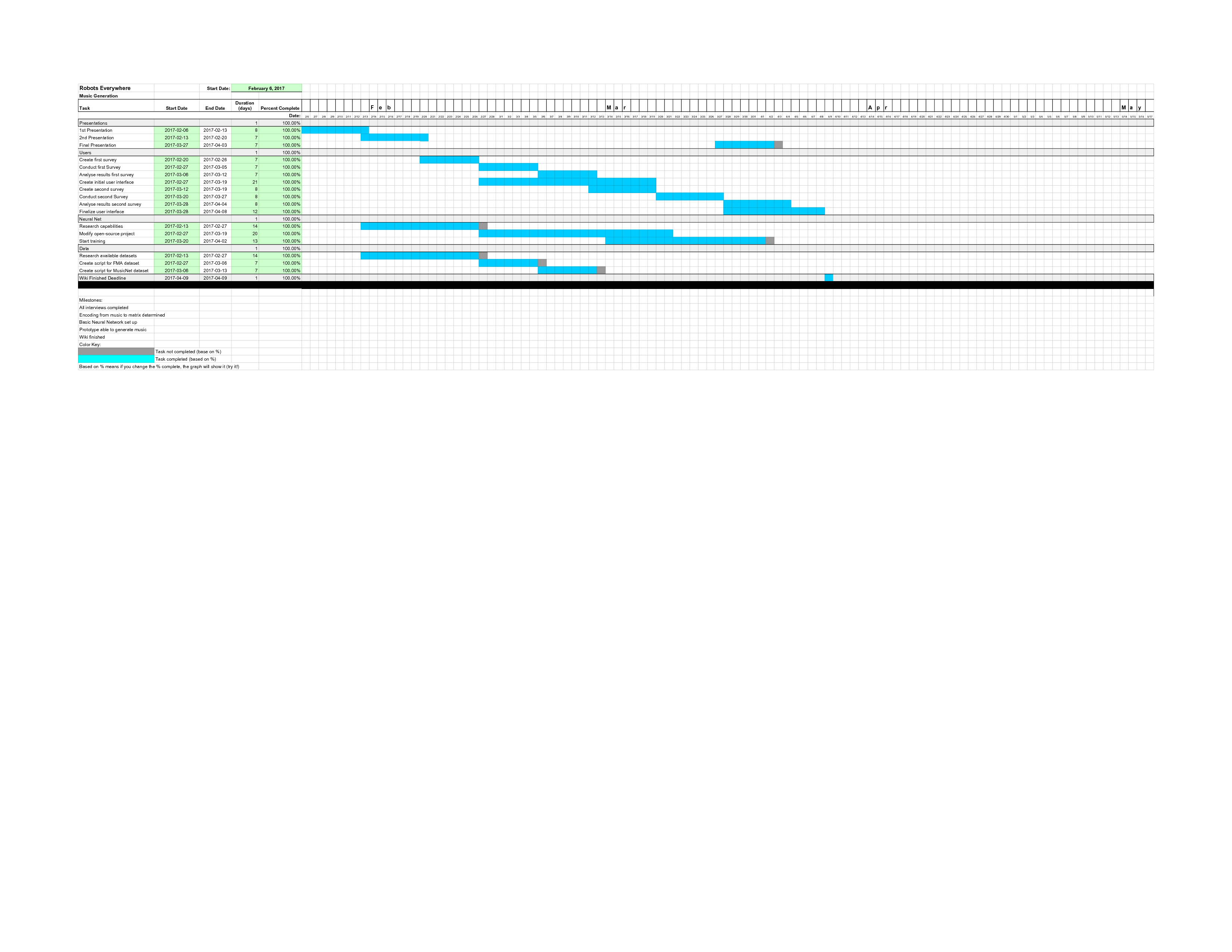
This Gantt chart is created to keep this project organized. It shows in which activities this project consist, when these activities take part and when an activity needs to be finished. During the course, the percentage of completeness in this Gantt chart will be updated.

week 1

• Decided on music generation as topic
• Clarify USE aspects of the project
• Working on first presentation

week 2

• First presentation done
• Working on second presentation
• Created a project plan
• Created a task division
• Start researching available datasets
• Start researching neural nets

week 3

• Second presentation done
• Reworked project based on feedback
• Create questionnaire for survey
• Selected the datasets (FMA and MusicNet) to create scripts for
• Selected the open-source neural net (StackGAN) to build the project upon

week 4 (Carnival Week)

• Conduct survey
• Start working on the StackGAN codebase, with as first step understanding the project structure and getting the original version to work. Start postulating possible approaches to adapting the StackGAN code
• Begin user interface (website)
• Start creation data extraction script for the FMA dataset

week 5

• Analyse results from survey
• Modify StackGAN network structure to see how it adapts to selected approaches
• Script for FMA dataset done
• Start creation data extraction script for the MusicNet dataset

week 6

• Created 3 test setups for MusicGAN
• Continue implementing approaches for MusicGAN and experimentally check and fix the code
• Script for MusicNet dataset Done
• Fleshing out user interface (based on survey results)
• Create second survey for the user interface

week 7

• Conduct second survey
• Train MusicGAN on local computers and start gathering results
• Try to obtain cloud computing resources with GPU’s

week 8

• Working on final presentation
• Analyze results second survey
• Try to train on cloud computers given appropriate progress for training on local computers
• Analyse results of training and adjust setups per approach, where possible

week 9

• Final presentation done
• User interface finished (Revised with second survey results)
• Tidy up wiki
• Document results obtained for the MusicGAN project

week 10

• Finished the wiki

Task Division

Neural Network

• Noud de Kroon
• Rolf Morel
• Bas van Geffen

Data Engineering

• Noud de Kroon
• Herman Galioulline
• Rick Coonen
• Jaimini Boender
• Steven Ge

Website

• Rick Coonen

Surveys/Public opinion

• Rick Coonen
• Herman Galioulline
• Steven Ge

References

- ↑ Cope, David. EMILY HOWELL. http://artsites.ucsc.edu/faculty/cope/Emily-howell.htm
- ↑ 2.0 2.1 2.2 Google Research. TensorFlow: Large-Scale Machine Learning on Heterogeneous Distributed Systems. Public white paper, 2015.
- ↑ 3.0 3.1 Goodfellow, Ian, Yoshua Bengio, and Aaron Courville. Deep learning. MIT Press, 2016.
- ↑ Mirza, Mehdi, and Simon Osindero. "Conditional generative adversarial nets." arXiv preprint arXiv:1411.1784 (2014).
- ↑ Denton, Emily L., Soumith Chintala, and Rob Fergus. "Deep Generative Image Models using a Laplacian Pyramid of Adversarial Networks." Advances in neural information processing systems. 2015.
- ↑ 6.0 6.1 Zhang, Han, et al. "StackGAN: Text to Photo-realistic Image Synthesis with Stacked Generative Adversarial Networks." arXiv preprint arXiv:1612.03242 (2016).
- ↑ http://colah.github.io/posts/2015-08-Understanding-LSTMs/img/RNN-unrolled.png/
- ↑ http://colah.github.io/posts/2015-08-Understanding-LSTMs/img/RNN-longtermdependencies.png
- ↑ Hochreiter, Sepp, and Jürgen Schmidhuber. "Long short-term memory." Neural computation 9.8 (1997): 1735-1780.
- ↑ http://colah.github.io/posts/2015-08-Understanding-LSTMs/img/LSTM3-SimpleRNN.png
- ↑ http://colah.github.io/posts/2015-08-Understanding-LSTMs/img/LSTM3-chain.png
- ↑ 12.0 12.1 Eck, Douglas, and Juergen Schmidhuber. "Finding temporal structure in music: Blues improvisation with LSTM recurrent networks." Neural Networks for Signal Processing, 2002. Proceedings of the 2002 12th IEEE Workshop on. IEEE, 2002.
- ↑ 13.0 13.1 Eck, Douglas, and Jasmin Lapalme. "Learning musical structure directly from sequences of music." University of Montreal, Department of Computer Science, CP 6128 (2008).
- ↑ 14.0 14.1 https://magenta.tensorflow.org/
- ↑ Bertin-Mahieux, Thierry, et al. "The Million Song Dataset." ISMIR. Vol. 2. No. 9. 2011.
- ↑ Benzi, Kirell, et al. "FMA: A Dataset For Music Analysis." arXiv preprint arXiv:1612.01840 (2016).
- ↑ http://colinraffel.com/projects/lmd/
- ↑ https://www.reddit.com/r/datasets/comments/3akhxy/the_largest_midi_collection_on_the_internet/