Mobile Robot Control 2023 Group 16: Difference between revisions
| Line 120: | Line 120: | ||
'''Assignment 2: Calculate the filter prediction''' | '''Assignment 2: Calculate the filter prediction''' | ||
As can be seen in Figure 4, it creates an average arrow of all particles spread over the area. This average filter prediction is a good estimation of the robot pose as here there is no noise taken into account. | As can be seen in Figure 4, it creates an average arrow of all particles spread over the area. This average filter prediction is a good estimation of the robot pose as here there is no noise taken into account. | ||
[[File:G16 Loc2 2.png|thumb|Fig 4: Applying filter prediction]] | [[File:G16 Loc2 2.png|thumb|Fig 4: Applying filter prediction]] | ||
Revision as of 15:39, 4 July 2023
Group members:
| Name | student ID |
|---|---|
| Marijn van Noije | 1436546 |
| Tim van Meijel | 1415352 |
Practical exercise week 1
1. On the robot-laptop open rviz. Observe the laser data. How much noise is there on the laser? What objects can be seen by the laser? Which objects cannot? How do your own legs look like to the robot.
When opening rviz, noise is present on the laser. The noise is evidenced by small fluctuations in the position of the laser points. Objects located at laser height are visible. For example, when there is a small cube in front of the robot that is below the laser height, it is not observed. When we walk in front of the laser, our own legs look like two lines formed by laser points.
2. Go to your folder on the robot and pull your software.
Executed during practical session.
3. Take your example of dont crash and test it on the robot. Does it work like in simulation?
Executed during practical session. The code of dont crash worked immediately on the real robot.
4. Take a video of the working robot and post it on your wiki.
Link to video: https://youtu.be/4mXdJyXXidE
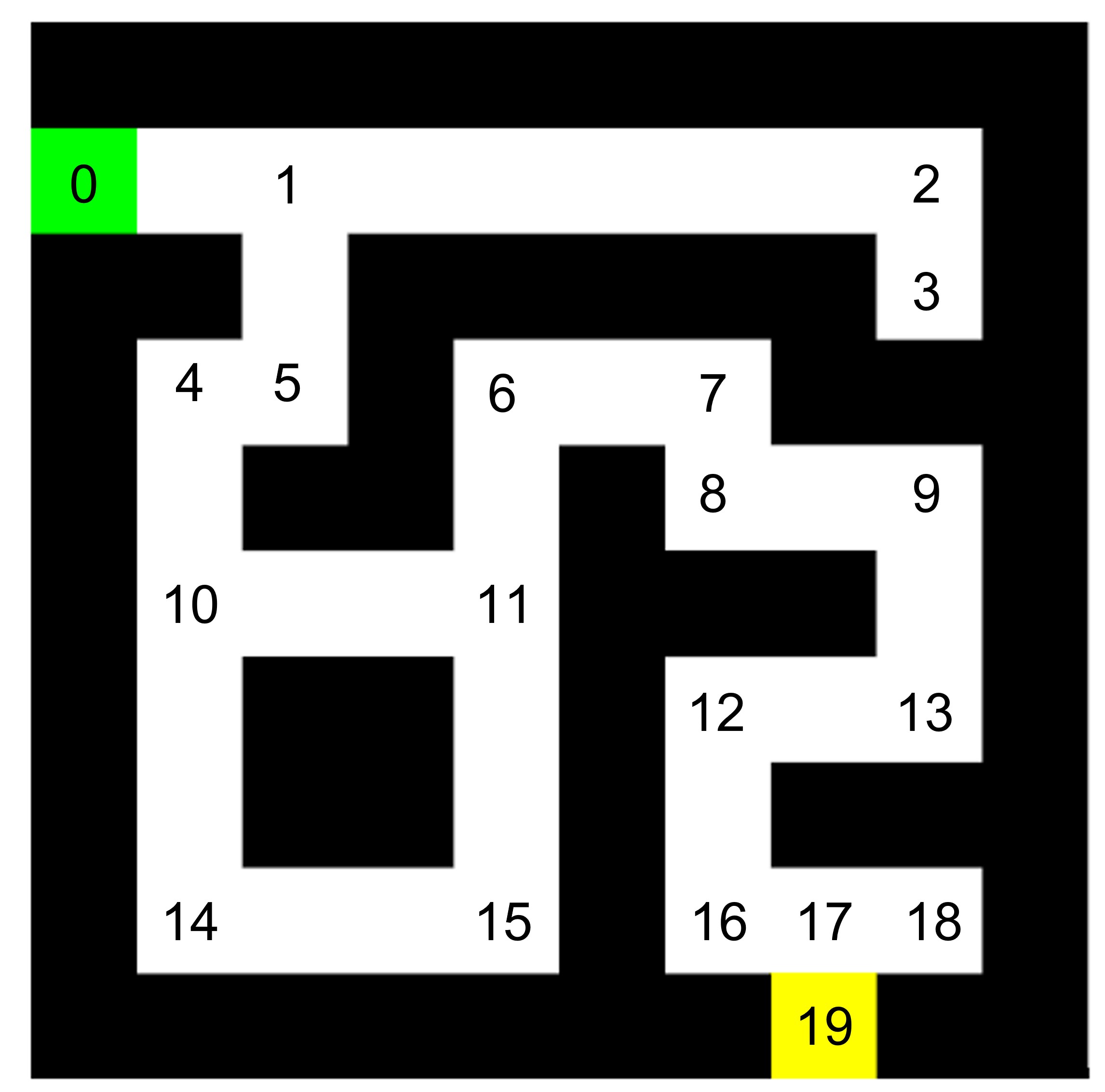
To make the A* algorithm more efficient, the amount of nodes should be reduced. This means that only nodes where the route change direction or where a path ends are considered. This is on the corners, T-junction and cross roads.
This would be more efficient, since the nodes in-between do not have to be considered by the A* algorithm. This increases computation speed.

To move the robot through the corridor, the Artifical Potential Field algorithm is used. There are two types of forces in this algorithm: the attractive force and the repulsive force. The attracting force calculated based on the position of the goal in comparison to the position of the robot. The repulsing forces are calculated by laserdata from walls and obstacles. When the robot moves forward in the corridor, it uses the laser to scan where the objects are positioned. Objects within a range of 1.5 meter are used in our approach. The repulsive forces result in a direction vector in which the robot wants to move. This direction is added up to the direction vector of the goal. Combined, these vectors result in a final direction vector in which the robot wants to move. The angular speed is then set to reach the desired direction.
Link to video of the simulation results: https://youtu.be/TG1GS70-G0A
Link to video of the real life experiment: https://youtu.be/_o3tM3mlx3E
Localisation assignment 1
Assignment 1: Keep Track of our location The code was written and uploaded on GitLab. It prints the odometry data including the difference between the last measurement and the new one.
Assignment 2: Observe the Behavior in Simulation
1) The accuracy of the odometry data is evaluated by running a simulation in which the robot has to follow a square path. The robot starts in the zero position. By following the path, the odometry data should constantly reflect the robot's exact position. Due to delays in the odometry data, the robot will probably never return exactly to its zero position, but when the odometric data return values of the actual position, it can be concluded that the accuracy is good. When the odometry data return values other than the position where the robot is actually located, the accuracy is no longer perfect.
2) When using the regular odometry data, the path followed is exact and after completing the path, the odometric data return the robot's exact position or at least know that the robot is not in the exact starting position. This can be seen in the video, where the robot ends slightly before the starting point, which can also be seen in the odometric data.
Using the uncertain_odom results in a similar final position. The uncertainty is not really visible. This is probably due to the low uncertainty level. However, in real life, this uncertainty will probably be larger.
3) No, we will not use this approach in the final challenge because in reality the same thing happens when using the uncertain_odom, but than also changing over time. The accuracy gets worse over time, so for the final challenge this is not desirable.
Video of simulation without uncertainty: https://youtu.be/DbtSd-Bld9s
Video of simulation with uncertainty: https://youtu.be/xS3cpYGw--8
Assignment 3: Observe the Behavior in reality
1) In reality, the robot has more uncertainties and if you run the experiment multiple times, the error changes each time you run the simulation. This means that you cannot rely on the odometry data. This is found in the video below. The robot ends up at the same position as it started. However, according to the odometry data, the robot is a bit in front of the starting position and turned to the right slightly. This is not the case in real life, and is caused due to wheelslip. This result was expected.
Video of real life experiment: https://youtu.be/e56ykR_f0xw
Localisation assignment 2
Assignment 0: Explore the code-base
What is the difference between the ParticleFilter and ParticleFilterBase classes, and how are they related to each other?
The ParticleFilterBase class is a base for the ParticleFilter class, as the name suggests. The ParticleFilterBase class consists of all basic functionalities the ParticleFilter uses. The ParticleFilter is initialised with specific values for the type of particle filter and the ParticleFilterBase consists of the underlying functions for the type of filter. This means the ParticleFilter is a initialised with the use of ParticleFilterBase.
How are the ParticleFilter and Particle class related to eachother.
The Particle class includes data of one particle. All particles are stored in a ParticleList. This ParticleList is used in the ParticleFilter.
Both the ParticleFilter and Particle classes implement a propagation method. What is the difference between the methods?
Both classes use a propagation method. The Particle class uses odometry data to propagate a particle, and takes process noise into account. The ParticleFilter class uses odometry data only, without including the noise.
Assignment 1: Initialize the Particle Filter
What is the difference between the two constructors?


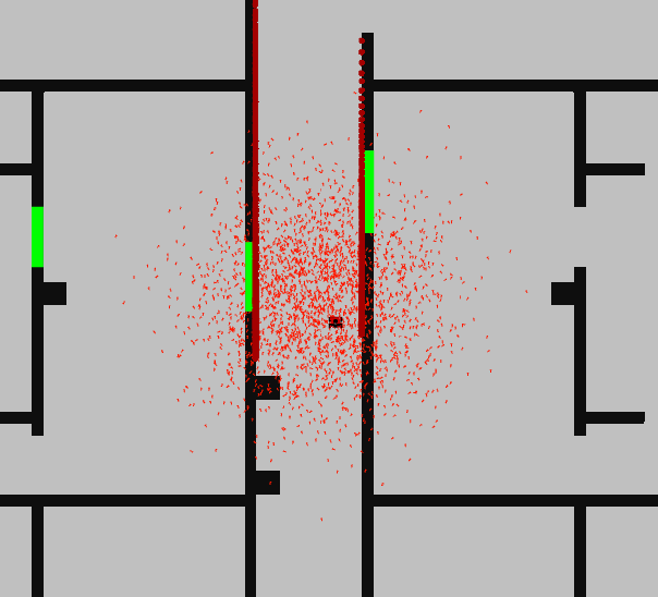
The difference between the two constructors is the fact that the first one creates a ParticleFilter with samples uniformly distributed along the environment. The second creates samples distributed according to a gaussion distribution.
Uniform distribution as shown in Figure 2
The advantageous of the uniformly distibuted constructor are that is easy to implement and most understandable, because it distribute its particles uniformly within a given space. Moreover, this method is less sensitive to extreme outliers. The disadvanteous of this method is that it could take longer to converge, which means that a lot of particles doesn't make sense to what we want to know, since they are uniformly spread over a large area. Also this method could be less precise, because of the equal probability of each particle.
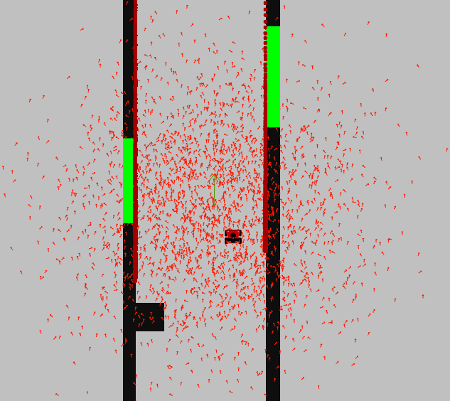
Gaussian distribution as shown in Figure 3
The advantageous of this Gaussian constructor is that this method is probably more precise, because of its underlying probability distribution. Moreover, this method will probably converge faster because it only need to focus on specific areas. The disadvantageous mainly focus on particles around the mean, which could cause that some spots in the area with lower probabilities are not taken into account.
If we for example are only interested in the regions in which we are likely to be, the gaussian (second constructor) will probably be the most efficient. If we do not know in which region we are probably be or we will sample everthing then the uniform (first constructor) will probably better.
Run demo1, open sim-rviz, and explain the results
In the figures the difference between the uniformly distributed particles and Gaussian distributed particles is clearly visible. In the uniform distributed particles the particles are divided over the whole area, while in the Gaussian method the particles are located around the robot. This is because the Gaussian method takes into account the probability of where the robot is likely to be.
Assignment 2: Calculate the filter prediction
As can be seen in Figure 4, it creates an average arrow of all particles spread over the area. This average filter prediction is a good estimation of the robot pose as here there is no noise taken into account.

Assignment 3: Propagation of Particles
Why do we need to inject noise into the propagation when the received odometry infromation already has an unkown noise component.
It is necessary to inject noise into the propagation because injecting noise is necessary to account for uncertainties and inaccuracies. Even if the odometric data already contain some unknown noise, this is often not enough to accurately represent the pose estimation by the particle filter. For example, the extra noise takes into account model inaccuracies of the robot, but it but also sensor noise or external disturbances. This means that implementing additional noise in this step will help to get a more accurate estimate of the robot position.
What happens when we stop here, and do not incorporate a correction step?
If the correction step is not included in the particle filter, the pose estimate is unlikely to be updated based on sensor measurements. If the correction step is skipped, no weights are assigned to particles based on measurements. This weight helps to concentrate particles around the actual pose and get a more reliable pose estimate from the robot. If the correction step is not performed, the robot's estimated pose will deteriorate over time and lead to a more uncertain and less accurate pose estimate.
Assignment 4: Computation of the likelihood of a Particle
The measurement model in the particle filter is used for the relationship between the robot's actual pose and the measurements taken. The likelihood function is needed to calculate how likely a measurement is given a guess about the robot's pose. This probability can later help assign how much weight to give each particle.
One possible problem that can occur is when multiple values between 0 and 1 are multiplied together to calculate the total value of the likelihood. This can lead to the total likelihood value becoming very small and being seen as 0 due to rounding. This is then not representative anymore.
Assignment 5: Resampling our Particles
The result is tested in the simulation. Testing in the map shows that this particle filter is a good approximation of the robot's pose. During testing, different options for particle amount and subsampling are tested to see what fits best. Increasing it a lot shows that it takes too much computing time, so it lags and is not representative. If you decrease it a lot, it does not represent the robot's pose well. The optimum is somewhere in between. What is really important to mention is that you need to have a good estimate of the robot's initial position, especially rotation.