Mobile Robot Control 2020 Group 3: Difference between revisions
No edit summary |
|||
| Line 325: | Line 325: | ||
===Rviz=== | ===Rviz=== | ||
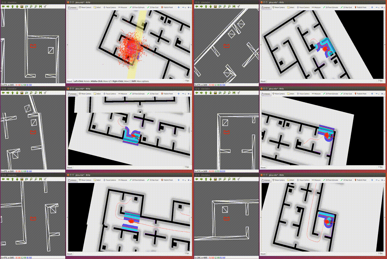
The visualization of the data from ROS is done with the built-in visualization tool Rviz. Rviz supports display of the provided map, cost-maps, laser, path data, transform frames, localization and pretty much any other topic, which can be represented visually. This is a great tool which has proven itself useful when debugging all sorts of issues, including localization errors, path planning issues, consequences of having the local cost-map update frequency set too low and global cost-map issues in logging the observed obstacles. Along side visual data, Rviz provides errors in a manner which is much easier to understand than reading debug logs saved by the terminal, since the errors immediately show up under the related topic. Additionally, it provides a graphic interface for users to input some rudimentary actions, such as localizing the robot and providing navigation goals. | The visualization of the data from ROS is done with the built-in visualization tool Rviz. Rviz supports display of the provided map, cost-maps, laser, path data, transform frames, localization and pretty much any other topic, which can be represented visually. This is a great tool which has proven itself useful when debugging all sorts of issues, including localization errors, path planning issues, consequences of having the local cost-map update frequency set too low and global cost-map issues in logging the observed obstacles. Along side visual data, Rviz provides errors in a manner which is much easier to understand than reading debug logs saved by the terminal, since the errors immediately show up under the related topic. Additionally, it provides a graphic interface for users to input some rudimentary actions, such as localizing the robot and providing navigation goals. | ||
==Hospital Challenge Demo== | |||
Figure 25 contains a GIF which shows the execution of the Hospital Challenge. [https://www.youtube.com/watch?v=YRWRkmJtT4o#file Click here for simulation video] where the robot shows it's ability to navigate through the hospital environment. | |||
[[File:demo.gif|1000px|Figure 25: A GIF of the execution of the Hospital Challenge.]] | |||
==Code snippets== | ==Code snippets== | ||
| Line 358: | Line 363: | ||
(Kalman Filter) http://robotsforroboticists.com/kalman-filtering/ | (Kalman Filter) http://robotsforroboticists.com/kalman-filtering/ | ||
Revision as of 18:39, 24 June 2020
Team members
M.N. de Boer (Martijn)
G.J.L. Creugers (Gijs)
P. Leonavicius (Pijus)
S. Narla (Shashank)
A.L. Nooren (Anna Lisa)
M.K. Salahuddin (Mohamed Kaleemuddin)
Design Document
In the design document the initial design ideas are elaborated for the topics requirements, functions, components, specifications and interfaces. In the next sections these topics are further explained, both the Escape Room and Hospital Challenge are taken into account. The Design Document can be downloaded here: Design Document.
Requirements
The requirements of a system are defined as the things the system should do. The requirements are divided into task performance, safety and software concepts. Where the task performance requirements include the requirements which needs to be resolved to be able to finish the Escape Room and Hospital Challenge. The safety requirements assure a safe execution of the challenges and the software requirements satisfy the an easy use of the software. The following requirements regarding the three topics should be satisfied by the simulated PICO robot:
Task performance
- The robot must be able to recognize target cabinets;
- The robot is capable of planning a path and is able to adapt its planned path to unexpected circumstances, for instance a closed door;
- PICO can rotate in place, in order to re-position when in front of a cabinet;
- Must be able to announce the completion of the current objective;
- The robot should not be inactive for more than 25 seconds;
- The robot has to be able to detect static and dynamic object and present them in the world model.
Safety
- The robot avoids collisions with static and dynamic obstacles;
- PICO must obey the limits on translation and rotation velocity;
- PICO should maintain a 5cm stopping distance from the obstacle.
Software
- The software is started by a single executable;
- The software can be easily updated;
- The User-interaction should be minimal and User-friendly.
Functions
The functions give a rough overview of how a successful execution of the challenges is break down into several sub tasks. The functions are divided into three subareas: input data processing, localization and control. The purpose of the input data processing functions is to process the raw data from the sensors (Laser Range Finder (LRF) and Odometer). After this processing, the raw data is converted to usable data for the other functions. In the localization function, the usable data is further processed towards a belief of the environment and is compared with what should be the actual environment. Also an actual position of the robot in the room is obtained. Finally, the control functions take care of the movement and positioning of the robot. The specific functions for a successful execution of the challenges are described in the next sections.
Input data processing
- Laser range finder interpretation
- The LaserData contains (range_min, range_max), which define what the smallest and largest measurable distances are. Furthermore, (angle_min, angle_max) determine the angle of the first and last beam in the measurement, (angle_increment) is the angle difference between two beams. This data is interpreted in this function and forwarded to the environment mapping functions.
- Odometer interpretation
- The OdometryData contains the displacement (x,y) and rotation (a) of the robot since its start, according to the wheel rotations. This displacement has to be interpreted and converted towards a position value of the robot, which is forwarded to the environment mapping functions.
- Sensor Fusion
- Combining sensory information from the LRF and Odometer sensors can result in a conflicting outcome, for example there can be a conflict about the exact location of the robot. This function can help to have reliable information flow to correlate and deconstruct data.
- Vector map data interpretation
- A function used for structuring data obtained from the provided map of the testing area. To be used as inputs for position estimation and path planning functions.
Localization
- Environment comparison and localization
- This function will make a features based comparison between the expected surroundings based on the vector map and the output of the LRF interpretation function. The function will return the location of the robot (x,y,theta) coordinates on the map. A specific declaration of the to be used coordinate system needs to be further defined.
- Obstacle recognition
- Together with the environment comparison, obstacles has to be recognized. This function determines if a feature obtained from the LRF interpretation function is either a known wall or a unknown obstacle. The comparison will be done in the same manner as the environment comparison, feature based. If an unknown obstacle is determined, it has to be marked as such.
- Position estimation
- Once a location is obtained from the Environment comparison and localization function, the location has to be compared with the OdometryData. After this comparison the robot has the final belief of where it is in the room and the control functions can take care of the movement and positioning of the robot.
Control
- Path planning
- A function based on a Dijkstra’s/ A* / Dynamic programming algorithm. Uses data from the provided vector map and outputs from LRF and Odometry interpretation functions. Constantly recalculates the optimal path based on detected obstacles or changes in the environment such as closed doors. However the interpretation functions return a feature based interpretation of the environment there is chosen to not do a feature based navigation. On the other hand, there is chosen to implement a path planning algorithm to have a more efficient routing through the rooms (in case of the Hospital Challenge). The specific algorithm for path planning has to be considered.
- Movement functions
- This function is used for describing routines to be sent as inputs for the base controller of the robot.
- Final re-positioning
- After the objective position is reached, the rotation of the robot is compared to the required value obtained from the vector map data. Furthermore the function contains a robustness check for the Hospital Challenge, if the robot has the belief it is aligned towards the cabinet there is a check with use of the LRF data if it is actually correctly aligned towards the cabinet. For example, there can be a check if the feature in front of the robot is perpendicular to the front beam of the LRF.
- Signaling function
- The decision making process of completing a objective is printed on the screen. In this way there can be tracked in which phase of decision making the robot is in, which makes ambiguities in the process more visible to the user. Furthermore. a print output marks the completion of an objective: called once the final state of the path planning algorithm is reached and the correct orientation of the robot is achieved.
- Safety function:
- Constantly running in the background (as a separate process/thread) in order to detect anomalous behavior of the mobile robot and interrupt the operation of the robot if necessary.
Specifications
The specifications of a system are defined as the specific things the system really can do. In this case specifications are the things PICO is capable of regarding speed limits and specific functionalities which are imposed by both the Escape Room and Hospital challenge.
- Maximum speed of 0.5m/s translational, 1.2rad/s rotational;
- Maintain a distance of 20cm between walls and PICO to make sure the walls will not be bumped, stop and reroute if distance is less than 20cm;
- Maintain a distance of 80cm from any dynamic object to consider the movement of those objects;
- Move at a maximum speed of 0.3m/s while tracking a dynamic object;
- Move forward slightly, if robot has been standing stationary for 30s;
- Position PICO π rad with respect to the cabinet upon arrival;
- Visit the cabinets in the required order.
Components
The components give a overview of the hardware of PICO, containing the sensors, actuators and computation unit, a global outline is given in this section.
Sensors
- Laser Range Finder
- Provides a set of points in polar coordinates relative to the PICO robot.
- Wheel encoders
- With this distance translated and rotated can be measured, is however highly sensitive to noise and will require filtering.
Actuators
- Holonomic base wheel
- It can realize the required degrees of freedom - translation in x and y and rotate about the z-axis without any position level constraints.
Computation unit
- This contains the software module that drives the robot and lets all other components communicate.
Interfaces
In this section the interface design for the robotic system is displayed. The interface shows the boundary between the components of PICO (Laser Range Finder and Odometer) and the exchange between the software components Localization, Control and Actuation. The interface design is shown in Figure 1.

Escape Room challenge
For the Escape Room Challenge a wall-following algorithm has been implemented. This algorithm consists of multiple phases, these phases are visualized in Figure 2.

Phase 1
Since the robot is not aware of its initial position first a wall has to be found before the actual wall following can happen. This is done by driving in a straight line until a wall is detected in a cone of the LRF facing forward. When a wall has been found the software switches to phase 2.
Phase 2
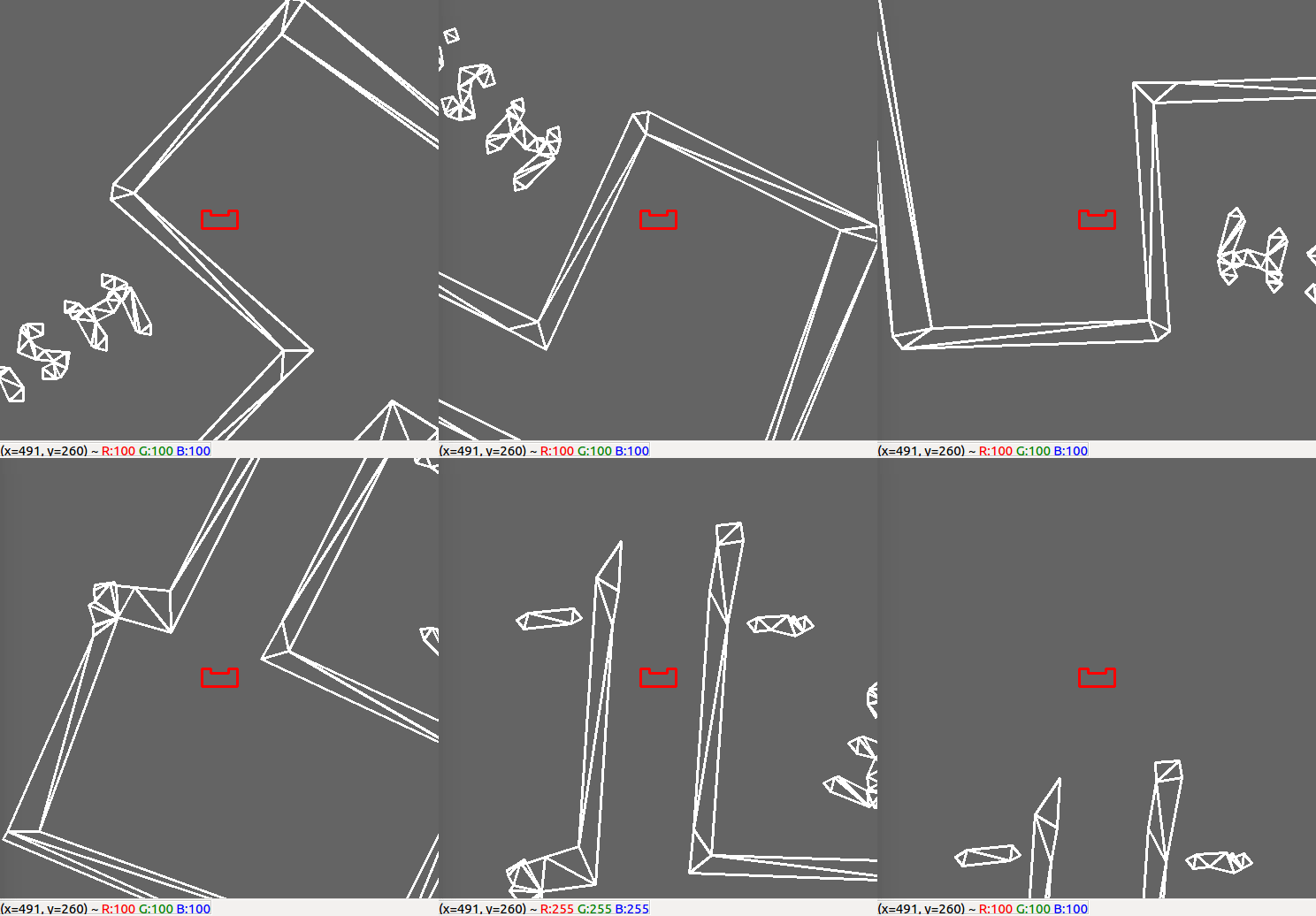
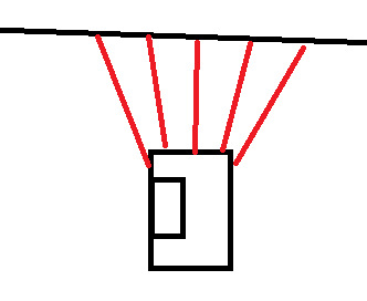
Now that a wall has been localized the next thing is to align the robot parallel to the wall. The estimation of the angular position is done by comparing the values of a number of beams from the Laser Range Finder. In order for the robot to be parallel to the wall, the beam perpendicular to the robot must detect something closer than beams that are ten beams more to the back and to the front. Those beams have to detect some thing closer that beams 10 more beams to the back and front. This condition is illustrated in Figure 3. The robot will rotate until this condition is true, then it will move to phase 3.
Phase 3
In phase 3 the robot will drive along the wall while looking for the exit. In this phase two things can happen. First the robot might sense an obstacle in a cone in front of it and switch back to phase 2. Then it will either align to the current wall if it was driving into it (possibly because of drift) or it will align to the new wall, since a corner has been found. The other option is that a cone to the right of the robot detects no wall, as in Figure 4. This means that the exit has been found and thus the robot switches to phase 4.
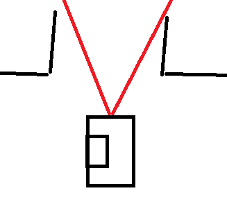
Phase 4
Phase 4 takes care of aligning with the exit of the escape room. This is done by rotating the robot until a determined cone of lasers in front of the Pico does not detect a wall anymore. When this is the case it will move to phase 5.
Phase 5
In this phase the robot will move in a straight line trough the corridor until it reaches the end. It will switch to phase 6 when the outermost laserbeams at either side do not detect any walls anymore.
Phase 6
When the robot reaches the end of the corridor it switches to phase 6 which will stop the movement to make sure it does not keep going to infinity and beyond.
Result Escape Room Challenge
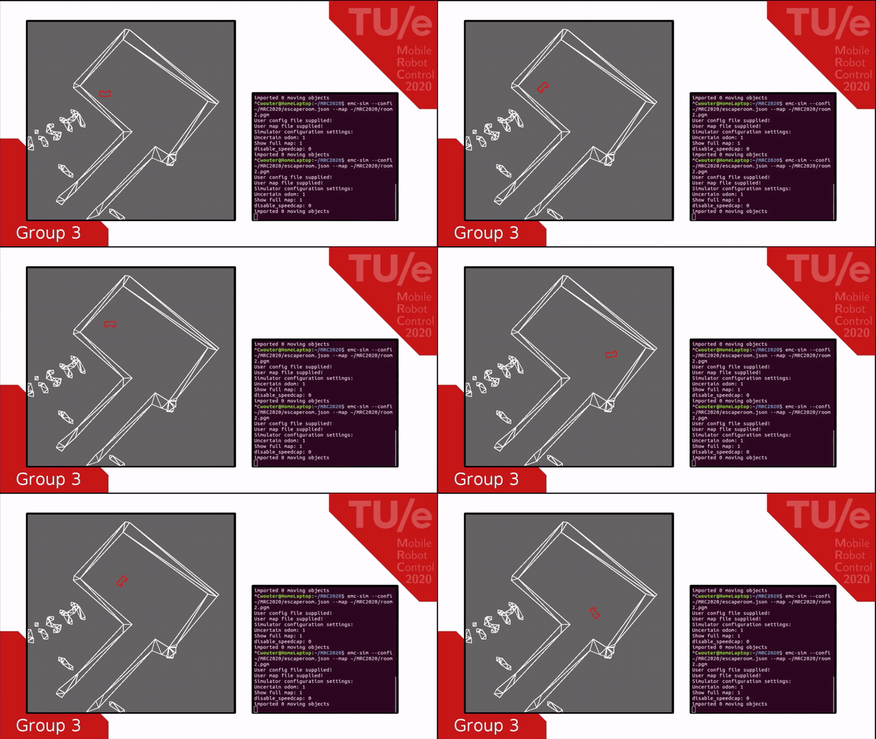
Figure 5 is a GIF of the actual Escape Room Challenge where the robot failed to exit the Escape Room. This was due to a minor bug in the software. In self drawn maps, the corridor outwards was not as long as the one from the actual Escape Room. Therefore PICO did not detect it when it was not close enough to the exit, as the cone would be interrupted by the side of the wall. The roaming nature of the algorithm however made sure it was close enough to the exit. Resulting in this cone being uninterrupted and thus PICO being able to proceed to the next phase. However, in phase 4, the algorithm did also have a too large cone forward where no obstacle should be detected in order to proceed to the next phase, resulting in PICO perpetually rotating. This cone was changed from 160 to 36 lasers wide. This little fix results in PICO being able to leave the room, as showed by the GIF in Figure 6. The snippet with the correct code can be found here Escape room challenge.
-
Figure 5: A GIF of the execution of the actual Escape Room Challenge, broadcasted on YouTube on the 13th of May, 2020.
-
Figure 6: A GIF of the execution of the Escape Room Challenge after the cone size for aligning PICO to the exit was reduced.
Hospital challenge
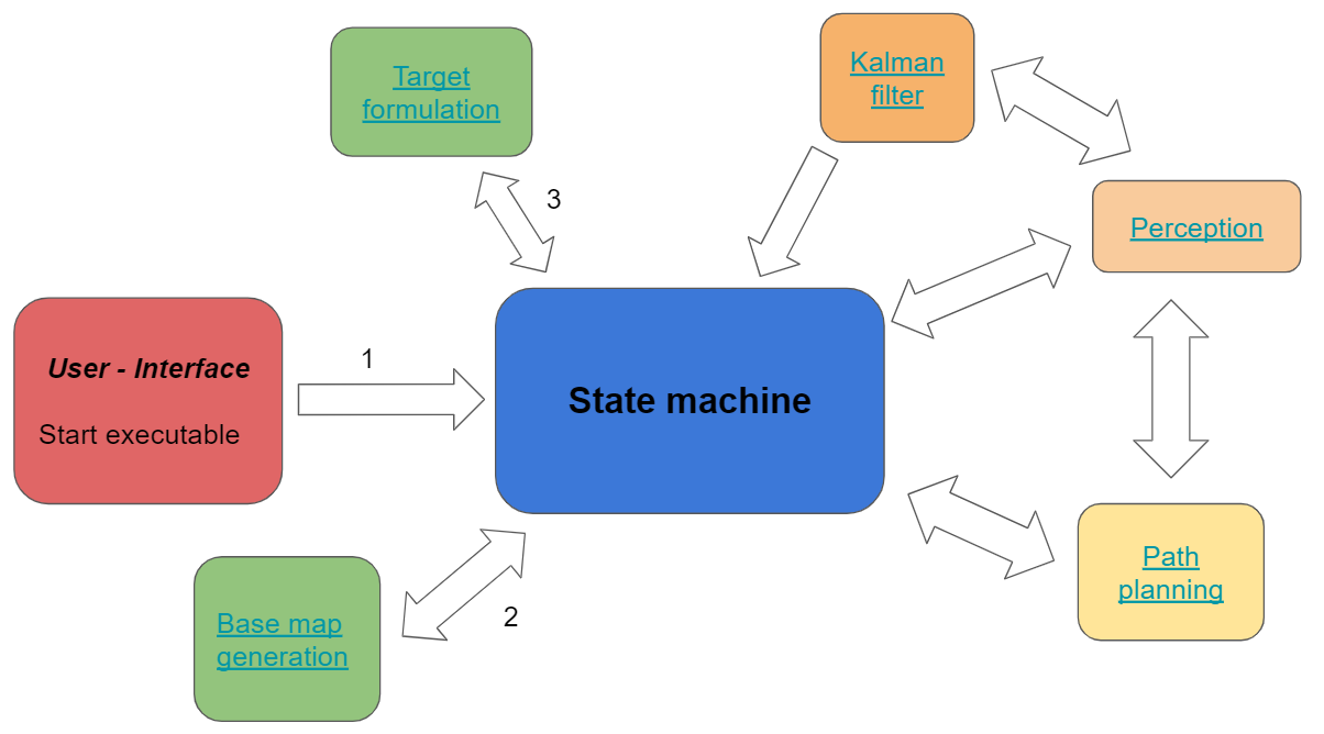
In the Escape Room Challenge the simulation environment has been explored in a relative simple fashion. The Hospital Challenge is obviously more advanced, but some modules can be adjusted and used again. A schematic visualization of the state machine for the Hospital Challenge is shown in Figure 7. The separate modules will be elaborated in the next paragraph.
Base map generation
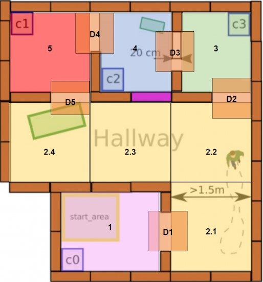
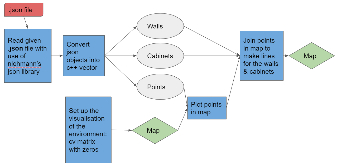
Initially it was the idea to divide the map into multiple areas and follow the robot from start to target in a state machine. This in order for when the robot encountered an obstacle, it can follow the state machine in the physical world for a new path. An example of this division and state machine is given in Figure 8 and 9. Note that areas 2.2 to 2.4 in Figure 8 can be merged into one area, since they do not represent changes in the state machine, also doors can be omitted. However, there is chosen to do a more feature based map generation, since the pre-known layout of the hospital is given to the system in the form of a .json file. From this .json file features like walls, cabinets and points are extracted and converted into arrays. Using the data of the points, the arrays of the walls and cabinets were transformed into global coordinate form. In the section on target formulation it is more elaborated upon how this is done. In Figure 10 it is also shown in a schematic and what the idea was for visualizing the map.
-
Figure 8: A division of a room into multiple areas, splitted into seperate rooms and the hallway (which can be divided into areas of the same size as the other areas).
-
Figure 9: Representation of the state space in which PICO is located.
-
Figure 10: Schematic view of how the .json file is converted to a visualization of the map.
Grid development
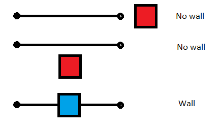
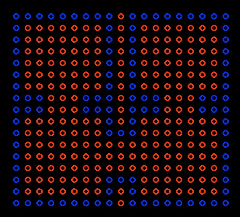
In order to make a grid to feed to the A* pathplanning algorithm, a gridpoint array is made using a discretization factor D (which denotes the size of the individual squares of the grid). This algorithm uses the x and y coordinates of the grid points and the ends of the walls in order to determine whether or not a wall crosses a grid point area. I order for this to be true, the coordinates of the wall must be within the grid square dimensions (a square defined by gridpoint-0.5*D to gridpoint+0.5*D in both directions) in one direction and bigger and smaller in the other direction. If one of the walls meets the condition, the rest of the walls don't need to be checked, in Figure 11 this is elaborated. In Figure 12 an example of a resulting grid map is given, each circle denotes a grid square and blue circles are walls. The code to make this map is given here: Grid map generator. However, making a gridmap ultimately proved unneccesary, as the A* algorithm that it was made for appeared to cause implementation issues and the ROS navigation stack just needed an image file to work. Therefore, since the ROS navigation stack had its own ways of determining a global path, the division into states and generating a state machine idea was also abandoned.
-
Figure 11: Elaboration of when the walls need to be further checked or not.
-
Figure 12: Example of resulting grid map, each circle denotes a grid square and a blue circle denotes a wall.
Perception
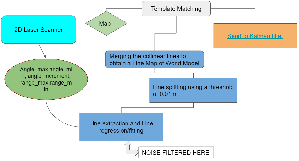
Perception is a process where sensory data is interpreted and used to understand the presented information of the environment. In this case it is used to obtain the specific location in the room from the laser scanner data. The perception process is showed in Figure 13 and contains the implementation of a Split and Merge and Template Matching algorithm. After the Template Matching algorithm, a (x,y, theta) location on the map is send to the Kalman filter to compare the obtained location from the laser scanner data with the location from the odometry data. After this comparison, the output will be a (x,y,theta) location of the robot in the room. In the next sections the to be used Split and Merge and Template Matching algorithm are discussed.
Split and Merge Algorithm
This most important module for the robot is to uniquely identify itself inside the map with a certain position and orientation (x,y,theta). There are multiple ways of doing this:
1. Dead-reckoning — a method that uses odometry data.
2. Landmark positioning — finding the exact position by measuring the distance to obstacles in the environment.
3. Sensor-based navigation — utilising a variety of range scanners to build a map of a visible area. Then it is compared with the global map to find the current position.
Since we did not have access to the map until a week before and we do not have GPS or vision system, there is proposed to use a combination of 1 and 3. The LRF data is used to extract valuable information such as lines and corners. There is planned to use the Split and Merge algorithm in order to generate a local map of what the robot perceives. This map will then be compared with the global map using template matching to get an estimate of the robot's position and orientation. The algorithm that is used for this was found in the Autonomous Mobile Robots course offered in Eth Zurich [1]
Firstly the Polar coordinates are converted to Cartesian coordinates (x,y) = (r*cosa,r*sina), where r is the range of the product and a is the angle that can be obtained by a = angle_min + (array index)*angle_increment. After converting the individual points to Cartesian coordinates, one can now try and represent these points into its line equation: ![]()
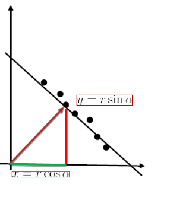
The r and alpha that fits these points into a line needs to be obtained. This particular process is called line fitting which is carried out by the fitline() function from the code snippet. This function is trying to reduce the least square error between the individual points (xi,yi) and the line equation that represent the line passing through this point. Which is denoted below:
Hence by taking the gradient of the least square error with respect to r and alpha, the formula for r and alpha is obtained that best fits a set of points as given below:

This fitline results in many lines that are formed but when there is for example a corner ahead or an intersection then this would lead to multiple lines forming at that place and so in order to split these lines a function called splitlinerecursive() is used to do this operation to distinguish between multiple lines.
After creating multiple lines, the job is not done yet. We need to make sure that there is one unique line representing the points and not a multitude of lines spread across as points. So, we need to merge the collinear neighbours as shown in figure 15 and this is done by the function mergecollinearneighbours().
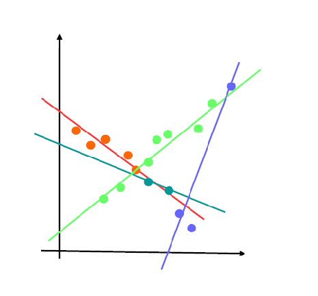
Finally the function extractlines() is called inside the loop of while(io.ok()) to perform the split and merge algorithm over every sampling time and store it in a matrix and send it to the template matching algorithm to give position estimates of pico.
Several issues were faced while trying to implement the split and merge algorithm on C++ because of passing multidimensional arrays to functions that modified the elements inside. We had originally tried using pointers and double pointers to access the elements but we had problems with accessing memory. We tried in all our efforts to make it work using external libraries but still we could not fix it. This made us drift towards implementing ROS packages.
Template Matching
The template matching algorithm is a widely used computer vision technique to find areas of an image that match to a template image. In the perception process the laser scanner data is processed to an image of the near environment, which is with use of the template matching algorithm matched to the known map of the room. For the implementation of the algorithm the OpenCV library is used, this library contains standard functions to perform the Template Matching method. To execute this method, two functions are of main importance: matchTemplate() and minMaxLoc(). The first function slides the template image over the source image and compares the template against overlapped image regions in the source image. There are six comparison methods defined to choose from, these are further defined in [2]. After the comparison is done, the best matches can be found as global maxima or minima, depending on the method. To find this specific maximum/minimum value the minMaxLoc() function is used. The function returns the the minimum and maximum element values and their positons. This position can be used as the top-left corner of the rectangle which represents the template image.
Kalman Filter
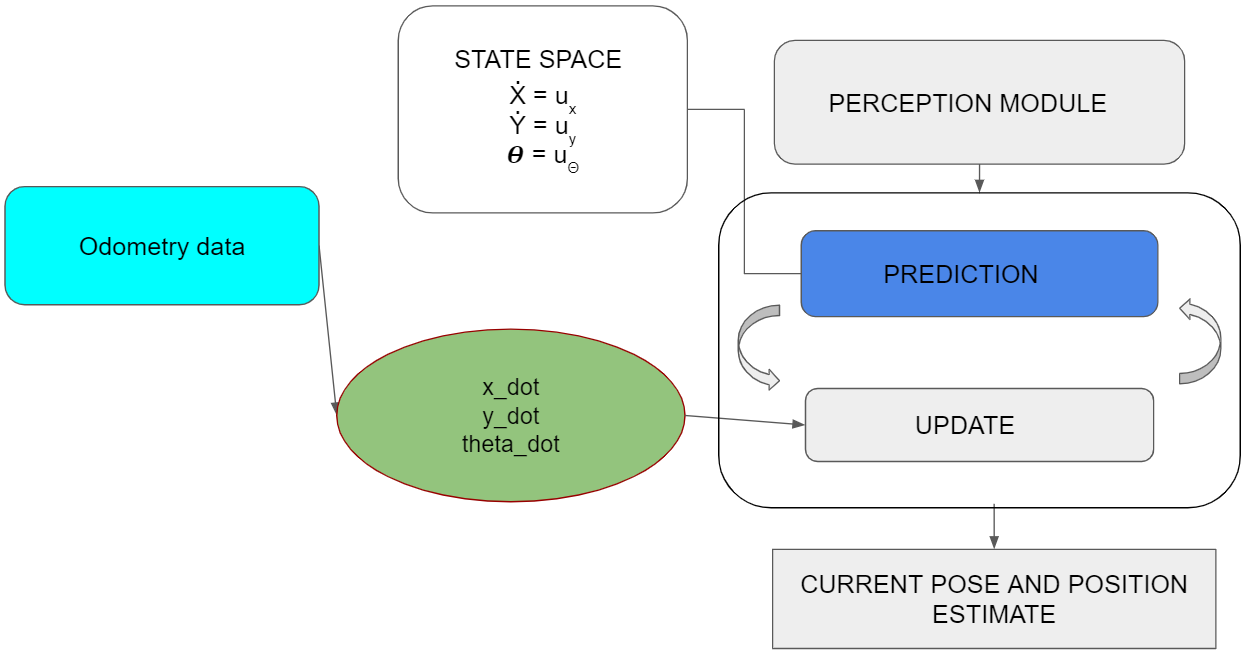
To merge the odometry data into position estimation a Kalman filter is implemented, a schematic representation is showed in Figure 16. The Kalman filter is a usual choice to filter the noisy signal from the odometry data that takes into account the uncertainty and gives close to accurate state measurements along with future predictions. Another benefit of the Kalman filter is that knowledge of a long state history is not necessary since the filter only relies on the immediate last state and a covariance matrix that defines the probability of the state being correct.
The Kalman filter depends extensively on linear algebra with it's prediction and update equations. C++ does not yet have a standard library to handle matrix operations as efficiently as MATLAB. Hence, to make the implementation easier, Armadillo [3] was used.The library can handle matrix operations through it's in-built classes. Since PICO robot is a linear system, the state space equations can be predicted easily. The noise covariance matrix and process covariance matrix are diagonal matrices that can be initially set to a predefined value and later converges to the correct value based on the Kalman gains. The equations are showed as follow:
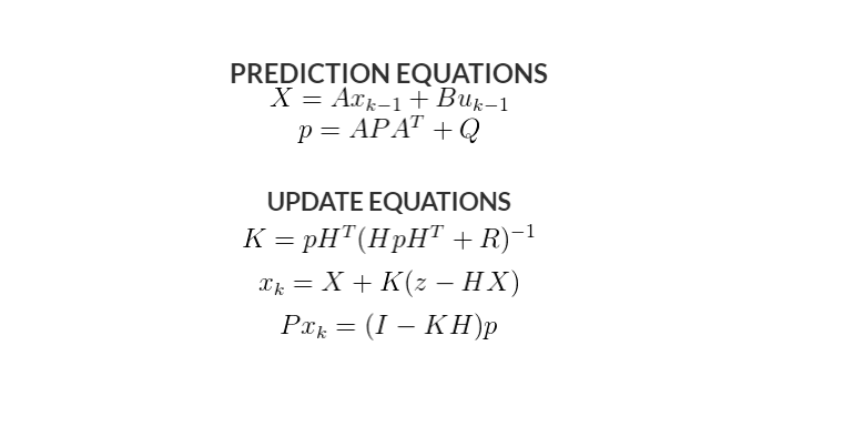
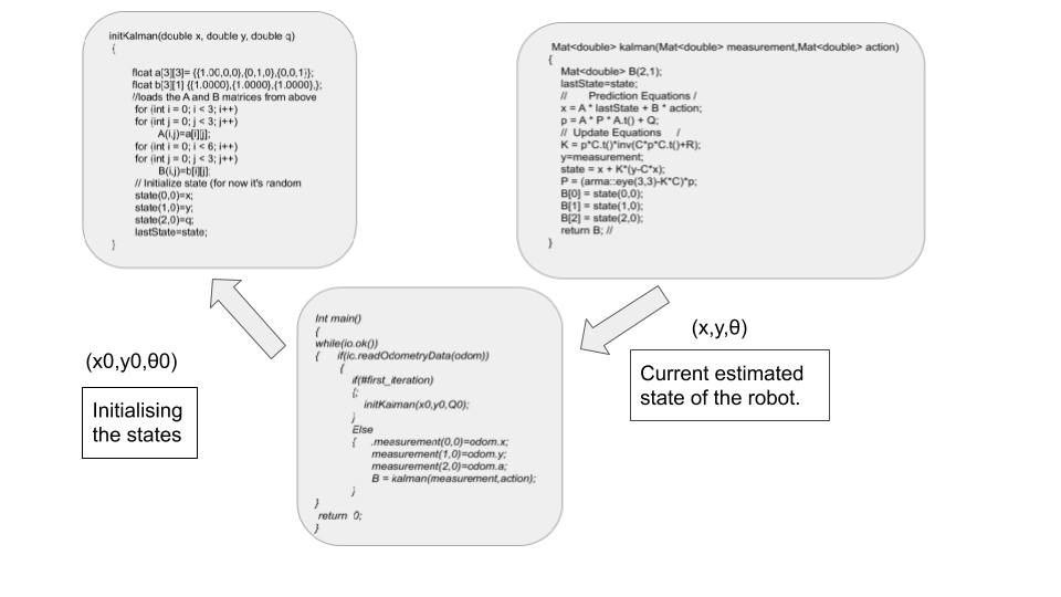
The Kalman filter implementation consist of two functions initKalman() and Kalman(), as showed in Figure 17. The function initKalman()initializes the state vector and also the A and B matrices for the Robotic system. Since the Robotic system is considered linear we have the standard state space equation x(k+1) = Ax(k) + Bu(k), Where A is an identity matrix of 3X3 and B is column vector of one. Note: The Matrices that have been defined here are matrices from an external library called Armadillo.
Target formulation
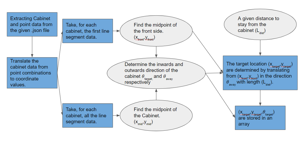
In order to make a good path from the start point to the first cabinet and so on, the pico needs to have a list of target positions it needs to visit. The process of determining this list is discussed in this section and showed in Figure 18. Firstly the point data from the .json file is stored in a 2-by-n array, where n is the amount of points in the .json file. The location in the array notes which point it is. After that the Cabinet data is stored in a three dimensional m-by-4-by-2 array, where m is the amount of cabinets. The first dimension being the cabinet number, the second dimension being the wall number of the respective cabinet and the final dimension being the points of that respective wall. Thus each cabinet is a bundle of 4 combinations of points.
After constructing the cabinet and point arrays, the point values are translated into their global coordinates, creating a m-by-4-by-4 array. Here the third dimension changed from 2 to 4 since each point contains an x and y value.
To determine the midpoint of the whole cabinet, the means are taken from all the x coordinates and y coordinates of the cabinet array respectively.. This then results in a m-by-2 array, containing the x and y coordinates of the cabinet. In order to determine the midpoint of the front of the cabinet, the means of the coordinates are taken from only the first wall of the cabinet, since the first wall is always the front.
To determine the direction outwards of the cabinet, the x and y coordinates of the mid point of the cabinet are subtracted from the coordinates of the midpoint of the front and are then normalized. The inwards direction is simply the inverse of the outwards direction.
The x and y coordinates of each target location is then determined by translating from the front of the cabinet in the outwards direction with a predetermined length. This length is taken to be 0.5 meter, since the pico is about a meter wide and thus it can freely rotate after confirming it has done its objective at the cabinet. The inwards direction is converted to an angle in radians and stored as the third coordinate of the target. Ultimately a m-by-3 array is made containing the x, y and theta coordinates of each of the positions in front of and looking at the cabinet.
When starting the pico an array of cabinet numbers is given. This array is an input of this algorithm. After the final array from the alinea has been made, a new array k-by-3 array (where k is the amount of target cabinets)is generated containing all the position coordinates of the target cabinets in the desired order. This array is then given to the next part of the system. The snippet containing the code is given here: Target formulation.
Path planning
During the course of this project several changes have happened to the way path planning was implemented. Firstly a separate C++ library for an A* algorithm [4] was adapted. Unfortunately implementation issues with C++ and OpenCV have stopped the group from using this algorithm. The choice was made to completely switch to using the ROS Navigation stack for all path planning purposes. The Navigation stack is an extensive collection of ROS packages meant to fully cover all path planning and obstacle avoidance problems, an overview of the path planning structure is given in Figure 19.
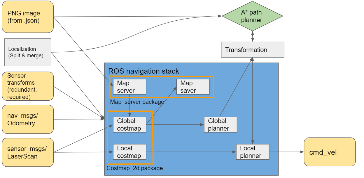
The default algorithms for path planning were used: Dynamic Window Approach (DWA) as the local planner and Dijkstra´s algorithm [6] as the global planner. An overview of these algorithms is provided below.
Local planner algorithm
DWA is an algorithm which works in the velocity space, and optimizes for circular paths only [5]. The algorithm uses known constraints of velocities and accelerations in order to calculate the appropriate path segment which will result in no collisions before the next recalculation is completed. An advantage of this algorithm is that it results in a slow movement when near obstacles or the final navigation goal, but a disadvantage is that only circular arcs are considered and in some cases this results in movements
Global planner algorithm
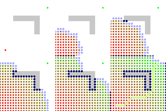
Dijkstra´s algorithm is a classical solution and is easy to understand, it computes the shortest path by evaluating and updating costs to each adjacent grid point on the known global cost-map. A graphical representation of the algorithm is presented in Figure 20. An important thing to note is that the global planner within the Navigation stack consists of two separate parts: the Dijkstra´s or A* algorithm, which computes the shortest path and a ¨potential field¨ calculation, which adjusts the path in order to take into account the known obstacles along with the defined inflation radius. There is a reason why Dijkstra´s algorithm is recommended in maps, which are not too large: due to the way Dijkstra´s algorithm works, a much larger potential field is calculated, when compared to A*, which provides more data for gradient descent optimization of the original path, this in turn results in smoother global trajectories.
ROS
One of the main challenges in this project was learning enough about the inner workings of the Robot Operating System in order to successfully implement the Navigation stack. This task took an immense amount of time even when one group member already had significant experience with using ROS. Due to a wrong conviction about coordinate transforms used by the AMCL package, the simulator was not made to work on time. Luckily the group was granted a special repeated challenge session one week later.
Localization
The original goal was to implement a Scan Matching algorithm paired with an extended Kalman filter to provide localization for Pico. Unfortunately this did not succeed and the choice was made to switch to the Adaptive Monte Carlo Localization package, which is an algorithm based on particle filters [8].
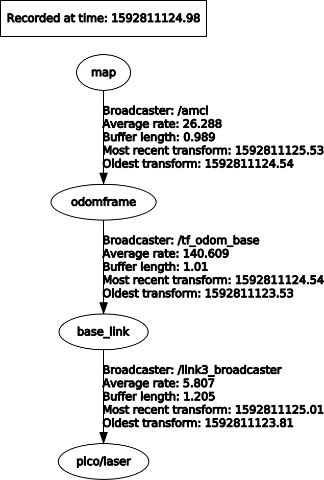
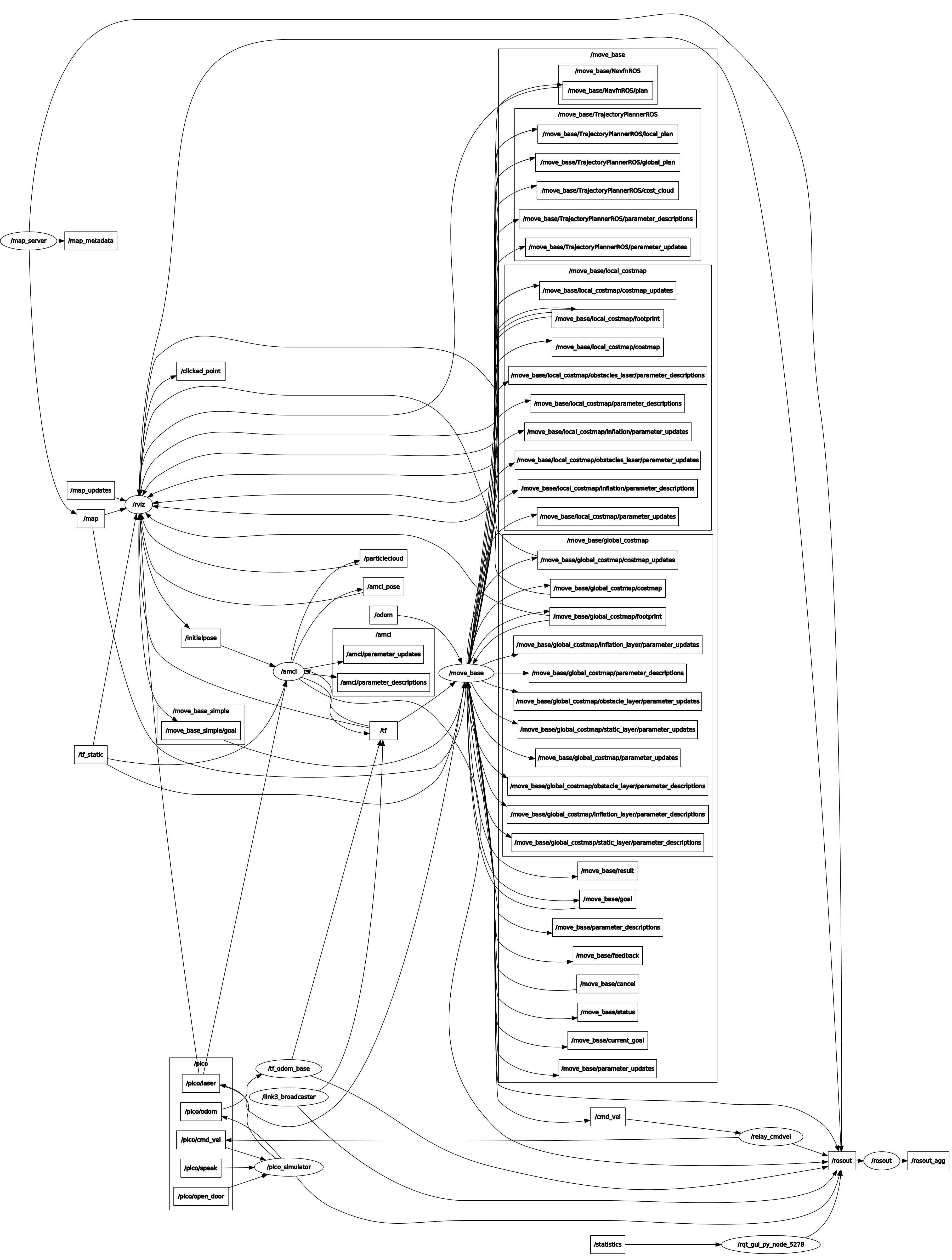
In order for AMCL to work, a few things have to be provided (AMCL Configuration): a laser scan message (sensor_Msgs/LaserScan) containing the laser range finder data, a known static map supplied by the map_server package (nav_Msgs/OccupancyGrid), an initial pose estimate message (geometry_msgs/PoseWithCovarianceStamped) and a correct transform tree message, which contains information on how to tie everything together (tf/tfMessage). The correct transform tree is shown in Figure 22 and the whole computation map showing interactions between all the present ROS nodes and packages is shown in Figure 24.
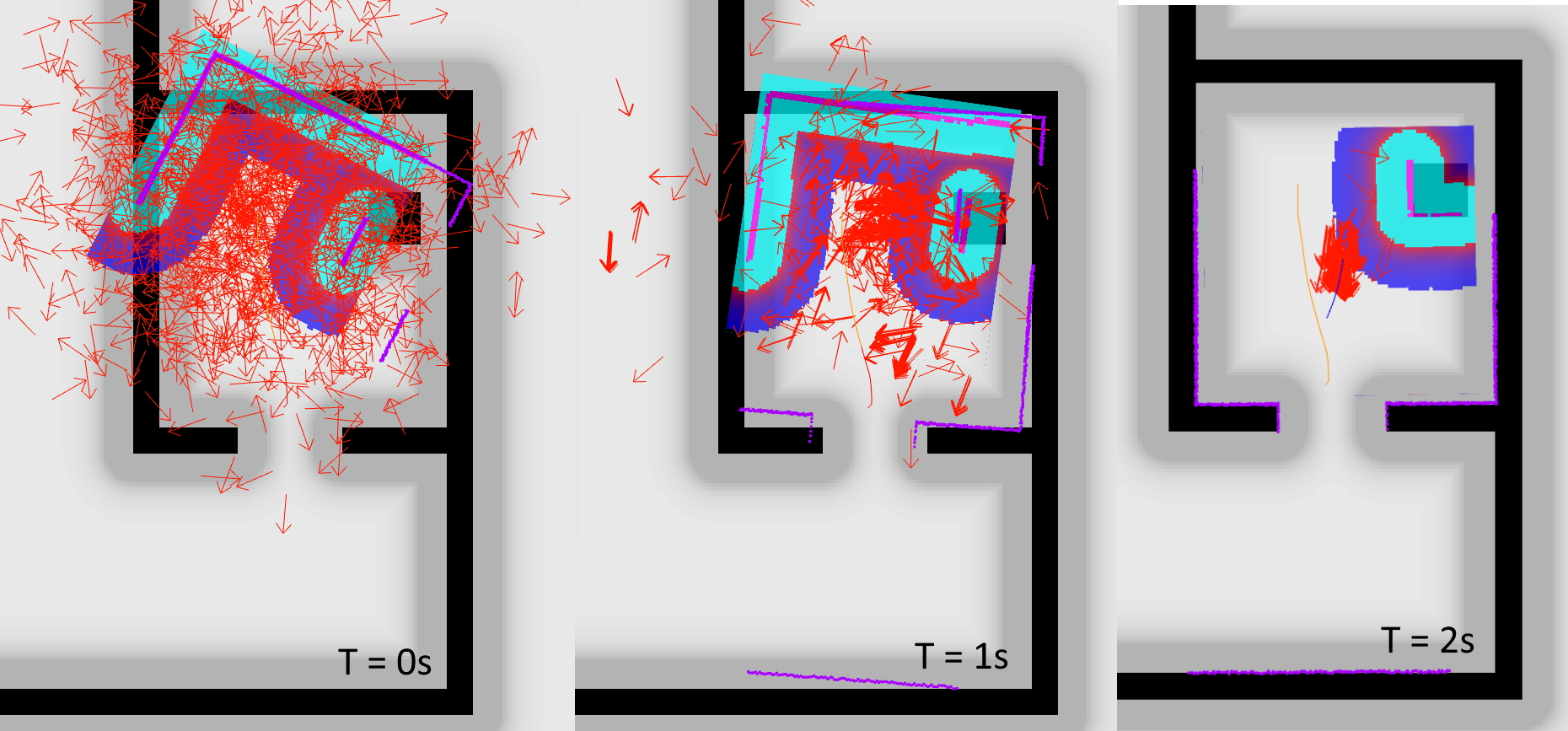
The issue, which was holding back the AMCL package from working is the transform frame between odometry data and the static map. We have successfully convinced ourselves that the odometry frame should be moving with the robot and its drift from the localized position would be provided by the AMCL package. Unfortunately this is a backwards way of thinking about this. The odometry frame should be entirely stationary with respect to the map frame, if odometry data was ideal and without drift and the AMCL package provides the drift between the map frame and the odometry frame. At first we had supplied a static transform between the odomeframe and base_link. The fix was to write a transform publisher, which would subscribe to nav_Msgs/Odometry and publish this data as a transform between the map frame and odomframe.
The starting area was known approximately, thus an initial pose estimate could be provided by choosing center of the start area as the inital coordinates. In order for localization to work suitable covariance values for x, y and theta values had to be provided. This allowed PICO to localize pretty quickly and start moving towards the goal, as showed in Figure 21. There was only one issue with this approach: if the navigation goal was close to the starting area of PICO (for example cabinet number 0), the robot would get lost, as it believed the goal was already reached before completing the localization.
Recovery behaviors
ROS Navigation stack incorporates two recovery behaviors: rotation in place and local cost-map clearing [9]. The initial recovery behavior is to clear the saved global cost-map updates (by default, any obstacle updates further than 3m away are eliminated). Unfortunately this first recovery behavior rarely improves the situation, it would be much more applicable in a real world scenario, where the cost-map gets cluttered with much more data, than in a simulation environment. After clearing the cost-map updates, Pico performs a rotation in place in order to clear out the surrounding space, lastly if this does not succeed, the final behavior is to completely clear the local cost-map and perform another rotation in place, which repopulates the local cost-map and hopefully results in a viable local trajectory being found.
Recovery behaviors are started if one of the following conditions are met: an oscillation is discovered, no global plan is received for a set amount of time or the local planner fails to find a valid velocity command for a set amount of time. In our case, recovery behaviors were started mainly due to the usage of the DWA algorithm for the local planner and sub-optimal settings for the cost map inflation. Pico would attempt to pass too close to the obstacles, which has a chance to result in the DWA algorithm planning a very small trajectory arc, which would be registered as an oscillation. After performing the first rotation in place, an acceptable trajectory was be found, but Pico would again attempt to pass too close to the obstacle thus repeatedly entering the recovery behavior. Unfortunately, during the final Hospital Challenge Pico got stuck in such a loop for more than a minute, thus resulting in a cancellation of the second challenge run. There are two main ways to circumvent this: increasing the inflation radius and adjusting the cost scaling factor parameter, but testing showed that adjustments of the cost scaling factor resulted in very minimal changes in trajectory and at the same time the inflation radius could not be increased, as that resulted in global path planning issues, which are discussed in the following paragraph.
Path planner issues
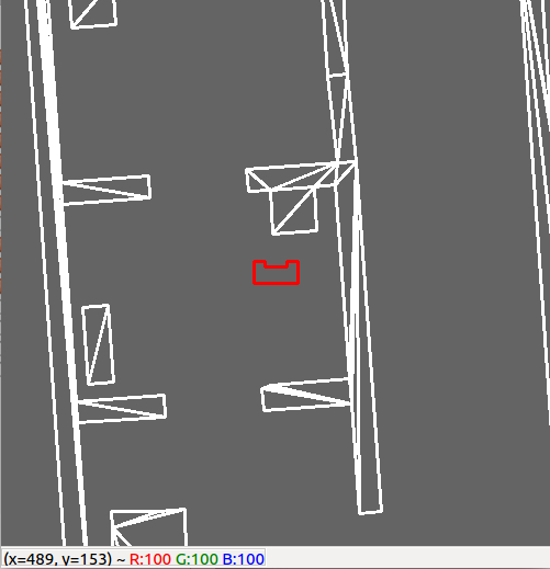
The inflation radius was set to 0.25 (while the Pico radius along the largest diagonal is equal to 0.224). The difference between the two radii is alarmingly small and as mentioned before it resulted in unwanted errors during navigation. The reason why this setting was used is tied to the navigation goals. The coordinates for target positions in many cases were rather close to the wall and if the target was placed within the inflation radius from a wall or cabinet, Pico would refuse to plot a global path and simply abort the whole navigation procedure. An attempt to remedy this error was made by adjusting the tolerance parameter of the global path planner, which seemed to work, but resulted in Pico plotting a path rather far away from the ideal position. A slightly exaggerated example of this is shown in Figure 23.
Cost-map
The costmap_2d package [10] is an integral part of the Navigation stack, which allows the robot to log the obstacles in its environment and update its path accordingly. When used through the navigation stack, the package automatically subscribes to the required transforms, simplifying the setup process greatly. A separate cost-map is used for local and global planning. The global cost-map starts out by applying the specified inflation radius to the provided map (if there is one), this is used as a baseline occupancy grid onto which any obstacles registered by the laser range finder are saved to. The local cost-map is a constant size square centered around the Pico, which is only used by the local planner to plot trajectories which avoid any logged obstacles.
The cost-map that was used for this project contains the following layers.
- Static Map Layer - contains the static map of the environment passed by user.
- Obstacle Map Layer - Contains the obstacles mapped with the help of laser data. This layer performs both operations: locating and saving the obstacles as well as raytracing through the observed area in order to remove previously logged obstacles which are no longer present.
- Inflation Layer - contains the inflation of the obstacles from static and obstacle map layer to provide accessible positions to the robot. This takes into account the specified inflation radius and the provided footprint of the robot. This layer is present by default and does not need to be specified.
The following parameters were used by both cost-maps:
obstacle_range: 10.0
raytrace_range: 11.0
robot_radius: 0.224
inflation_radius: 0.25
static:
   map_topic: /map
   subscribe_to_updates: true
obstacles_laser:
   observation_sources: laser
   laser: {data_type: LaserScan, sensor_frame: /pico/laser, clearing: true, marking: true,
   topic: /pico/laser, inf_is_valid: true}
Global Costmap
The following parameters were used to set up the global cost-map for the challenge:
global_frame: /map
robot_base_frame: /base_link
update_frequency: 2.0
static_map: true
plugins:
    - {name: static_layer,            type: "costmap_2d::StaticLayer"}
    - {name: obstacle_layer,          type: "costmap_2d::ObstacleLayer"}
    - {name: inflation_layer,         type: "costmap_2d::InflationLayer"}
Local Costmap
The following parameters were used to set up the local cost-map for the challenge:
 global_frame: /odomframe
 robot_base_frame: /base_link
 update_frequency: 5.0
 publish_frequency: 5.0
 static_map: false
 rolling_window: true
 width: 2.2
 height: 2.2
 resolution: 0.025
 plugins:
 - {name: obstacles_laser,           type: "costmap_2d::ObstacleLayer"}
 - {name: inflation,                 type: "costmap_2d::InflationLayer"}
Visualization
Rviz
The visualization of the data from ROS is done with the built-in visualization tool Rviz. Rviz supports display of the provided map, cost-maps, laser, path data, transform frames, localization and pretty much any other topic, which can be represented visually. This is a great tool which has proven itself useful when debugging all sorts of issues, including localization errors, path planning issues, consequences of having the local cost-map update frequency set too low and global cost-map issues in logging the observed obstacles. Along side visual data, Rviz provides errors in a manner which is much easier to understand than reading debug logs saved by the terminal, since the errors immediately show up under the related topic. Additionally, it provides a graphic interface for users to input some rudimentary actions, such as localizing the robot and providing navigation goals.
Hospital Challenge Demo
Figure 25 contains a GIF which shows the execution of the Hospital Challenge. Click here for simulation video where the robot shows it's ability to navigate through the hospital environment.
Code snippets
TF Publisher Escape room challenge Grid map generator Target formulation
References
[1] - Autonomous Mobile Robots course offered in Eth Zurich https://asl.ethz.ch/education/lectures/autonomous_mobile_robots/spring-2020.html
[2] - OpenCV documentation https://docs.opencv.org/2.4/modules/imgproc/doc/object_detection.html?highlight=matchtemplate#matchtemplate
[3] - Armadillo, C++ library for linear algebra & scientific computing http://arma.sourceforge.net/
[4] - A* algorithm https://github.com/SumiMakito/A-star
[5] - Fox, D.; Burgard, W.; Thrun, S. (1997). "The dynamic window approach to collision avoidance". IEEE Robotics & Automation Magazine.
[6] - Gass, Saul; Fu, Michael (2013). Gass, Saul I; Fu, Michael C (eds.). "Dijkstra's Algorithm". Encyclopedia of Operations Research and Management Science. Springer. 1. doi:10.1007/978-1-4419-1153-7. ISBN 978-1-4419-1137-7 – via Springer Link.
[7] - Visualization of Dijkstra's algorithm https://en.wikipedia.org/wiki/Dijkstra%27s_algorithm#cite_note-14
[8] - AMCL ROS package http://wiki.ros.org/amcl
[9] - Marder-Eppstein, E.; Berger, E.; Foote, T.; Gerkey, B.; Konolige, K. (2010) "Robust Navigation in an Indoor Office Environment" Willow Garage Inc., USA http://www.willowgarage.com/sites/default/files/icra2010_marder-eppstein.pdf(RECOVERY) http://www.willowgarage.com/sites/default/files/icra2010_marder-eppstein.pdf
[10] Costmap_2d ROS package http://wiki.ros.org/costmap_2d
(Split and Merge) M.Norouzi et al (2009) "Recursive Line Extraction Algorithm from 2D Laser Scanner Applied to Navigation a Mobile Robot".Proceedings of the 2008 IEEE
International Conference on Robotics and Biomimetics
(Kalman Filter) http://robotsforroboticists.com/kalman-filtering/
