Embedded Motion Control 2019 Group 3: Difference between revisions
| (314 intermediate revisions by 6 users not shown) | |||
| Line 22: | Line 22: | ||
|} | |} | ||
= | = Introduction = | ||
[ | This wiki page describes the approach and process of group 3 concerning the Escape room challenge and the Hospital challenge with the PICO robot. The PICO robot is a telepresence robot that is capable of driving around while monitoring its environment. In the Escape Room Competition, the robot is placed somewhere inside a rectangular room with unknown dimensions with one doorway that leads to the finish line. Once the robot crosses the finish line without bumping into walls, the assignment is completed. The Hospital challenge involves a dynamic hospital-like environment, where the robot is assigned to approach a number of cabinets based on a known map, while avoiding obstacles. | ||
The wiki is subdivided in the following parts: Firstly, the approach for the Escape room challenge is explained and evaluated. The second topic is the approach and evaluation of the Hospital challenge. This is followed by a full description of the system architecture used to perform the Hospital challenge. After the system architecture, the most important tests and test results are explained. Lastly, a conclusion and recommendation is provided. | |||
= Escape room challenge = | |||
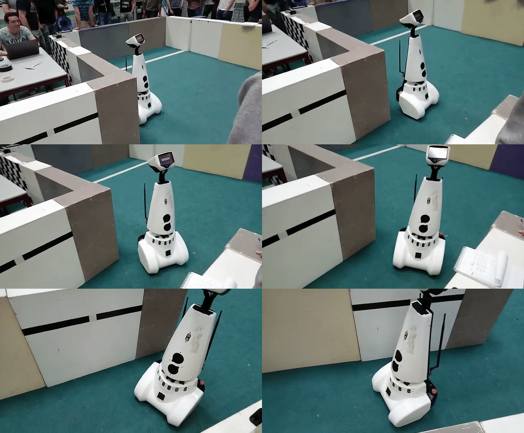
This chapter summarizes the approach for the escape room challenge and offers some reflection on the execution of the challenge. Figure 3.1 shows a small clip of our execution of the robot during the escape room challenge. | |||
[[File:EscapeRoom.gif|center|alt=Clip of group 3 at the escape room challenge|frame|Figure 3.1: clip of group 3 at the escape room challenge]] | |||
== Approach == | |||
The state chart in figure 3.2 depicts the wall following program that the robot is to execute during the escape room challenge. In a nutshell: the robot drives forward until a wall is detected, lines up with said wall to the right, and starts following it by forcing itself to stay between a minimum and a maximum distance to the wall. When something is detected in front, it is assumed that the next wall to follow is found, and thus the robot should rotate 90 degrees counterclockwise so it can start following the next wall. When a gap is detected to the right of the robot, it is assumed that the exit corridor has been found, and thus the robot should turn into the exit. Then the robot keeps following the right wall in the corridor until, once again, a gap is detected to the right of the robot. At this point, the robot should have crossed the finish line. | |||
[[File:EMC_2019_group3_ER_FSM.png|Figure 3.2: state chart Escape room challenge|center|thumb|1000px]] | |||
== Reflection == | |||
Due to a lack of time and more resources being put into the final challenge, the code for the escape room challenge had to be simplified. The original plan was to have the robot scan the environment, identify the exit, and when identified, drive towards the exit and drive to the finish line. In case the robot could not identify the exit, the robot would start following the wall instead, as a robust backup plan. The testing session before the challenge proved to be too short, and only the wall follower could be tested. Therefore, only the wall follower program was executed during the challenge. | |||
As a precaution to not bump into the walls, we reduced the speed of the robot and increased the distance the robot would keep to the wall by modifying the config file in the software. Although our program did succeed the challenge, we were the slowest performing group as a result of the named modifications to the configuration. We felt however that these modifications were worth the slowdown and proved the robustness of the simple approach our software took. | |||
= Hospital Competition = | |||
This chapter summarizes the approach for the hospital challenge and offers some reflection on the execution of the challenge. | |||
== Approach == | |||
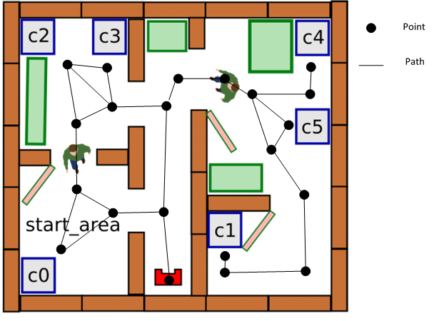
The general approach to the challenge is to create a point map of the map of the hospital. Figure 4.1 shows such a point map: | |||
[[File:Point_map_example.png|frame|center|Figure 4.1: example path point map]] | |||
A point is placed on different locations on the map. These locations are: at cabinets, on junctions, in front of doorways and in rooms. In the placement of these points, it is important that each point can be approached from a different point in a straight line. The goal of these points is that the robot can navigate from one side of the hospital to the other by driving from point to point. The points that the robot can drive to in a straight line from a point are its neighboring points. | |||
The original plan was to define the placement of each point by the distance and direction to its neighboring points and its surrounding spatial features. However, due to a lack of development time, it was decided to simply define absolute coordinates for each point. When the robot is on a point (A) and wants to drive to a different point (B), the robot can use the distance and direction to from A to B to drive to where B approximately is. Then, using the spatial features surrounding point B, the robot can more accurately determine its location compared to B and drive to B. For the path between points, it can be defined whether this path is through a doorway or hallway, or whether it is through a room. This can help in how the robot trajectory should be controlled during the driving from point to point. | |||
If the robots needs to drive from a starting point to an endpoint which is not neighbouring, the software will create a route to that point. This route is a list of points to which the robot needs to drive to get to the endpoint. To make sure the route is as efficient as possible, an algorithm is used which calculates the shortest route. The algorithm that is used is called "Dijkstra'a algorithm". A similar algorithm is also used in car navigation systems to obtain the shortest route. | |||
== Reflection == | |||
All sections of the final PICO program were operational and working in time for the final challenge. These together create a functioning solving plan as we had envisioned. This final program was tested in different simulation environments matching the final challenge. In the first simulation, a copy of the map of the final challenge was used, but without any static or dynamic objects, as wel as no closed doors. In this simulation everything was working very well, however, there was a chance that PICO could lose its position when it was doing its cabinet procedure. At the time of testing, the robot gets very close to the cabinet, and as a result, it sees a lot less of the room, which can cause the position estimation to act up. Other simulation tests used the same maps, but with added static obstacles and closed doors. In these tests it was noticed that the robot seemed to have more problems. The problems mostly arise from the robot losing its position due to matching the corners of static objects with points on the map. Doors also gave the added problem that a closed door may obscure corners that should actually be there. In general, we can determine that if the amount of visible corners gets too low, or there are too many wrong corners, the robot will lose its position. At that moment the position estimation code will try to fix this. This will work most of the time, but sometimes it will not be able to find the correct position again, or it will fix it in a completely wrong way. When that happens, there is no way to fix it anymore. By running these simulation tests a lot of time, we estimated that we had a 40% chance of completing the final challenge. | |||
During the final challenge, the robot had to visit the cabinets in order 0, 1, 3. The door was closed between 0 and 1, so the robot would have to find a alternative route between 0 and 1. Furthermore, there were some static obstacles, especially a big one in the hallway and in room 1, but less than we had anticipated. There was also one dynamic object, with which we had not run any tests beforehand, so we were not sure how the robot would react to that. Each group had two runs it could do. | |||
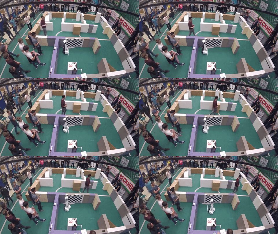
The first leg of the challenge went very well. The robot first had to determine its orientation, which it was able to do excellently during both runs. Figure 4.2 shows how PICO was able to determine its original orientation and how it corrects for this. | |||
[[File:orientation in start.gif|center|frame|Figure 4.2: hospital challenge - Finding initial orientation]] | |||
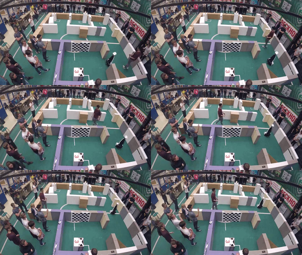
It will then go from the starting area to the hallway, from which it will go to room 2 and then end in room 0, as this route is the shortest route. Indeed, this is exactly what the robot did, as can be seen in figure 4.3. It went from waypoint to waypoint on the map, as we had defined it. It did so in a smooth manner, indicating that there were no issues with localization at this moment. | |||
[[File:from start to room.gif|center|frame|Figure 4.3: hospital challenge - Going from point to point]] | |||
When it arrived in room 0, it drove up to the correct side of cabinet 0, turned in the correct way, and drove up to the cabinet. This is shown in figure 4.4. In the first run, it did this in a correct manner, but in the second run, it did not drive close enough to the cabinet, and the jury was not sure if cabinet was correctly reached. | |||
[[File:cabinet procedure.gif|center|frame|Figure 4.4: hospital challenge - Cabinet sequence]] | |||
Next, the robot had to go to cabinet 1. Normally the fastest route would be going from room 0 to room 1, but the door between them was closed. So the robot had to drive to the door to notice this. At this moment the first problems with localization arose, in both runs. As we had noticed in the tests, the robot had difficulty estimating its position when it is located very closely to the cabinet, and while the robot was moving from the cabinet to the door, it first went the wrong way, towards the wall. It did this in both runs. In run 1, it merely scraped the wall, but in test 2, it bumped quite hard into the wall. The potential field should have stopped the robot from bumping into the wall, even though it lost its position, but this was not able to prevent it. In both runs however, the robot was able to fix its position eventually. | |||
It then drove up to the door, waited for a while, and then correctly determined that this door was closed. It was able to do this correctly in run 1, as displayed in figure 4.5. | |||
[[File:alternative route.gif|center|frame|Figure 4.5: hospital challenge - Finding an alternative route]] | |||
In run 2 the robot again lost its position at this instant, and again drove straight into the wall, knocking the wall completely out of place. This meant the end for the second run. In the first run however, it was able to keep its position, and go to the hallway again. This is shown in figure 4.6. | |||
[[File:going to hallway.gif|center|frame|Figure 4.6: hospital challenge - Going to next cabinet]] | |||
In the hallway it had to go from one end to the other, with one big obstacle in the way, and a person walking around the hallway. This proved to be too much for PICO, as it again seemed to lose its position. It tried to fix this, but it was not able to localize correctly anymore, which meant the end of the first run. This attempt is shown in figure 4.7. | |||
[ | [[File:losing its position.gif|center|frame|Figure 4.7: hospital challenge - Losing postion]] | ||
In both runs, the robot was able to find the first cabinet, complete the procedure there, and was able to determine another route because of a closed door. However, going from cabinet 0 to cabinet 1 proved too difficult for the robot, which mainly has to do with localization issues. This was something that we had anticipated, but we are very happy that PICO was able to show a correct first part in both runs. Localization seemed to be the biggest and most difficult issue to tackle, so more time could have been spent on this aspect of the program. | |||
One detail that was discovered after the challenge though, is that the snapshots that were supposed to be taken during the cabinet procedure were nowhere to be found in the project directory on PICO. That is a problem, as it was a requirement of the challenge to take snapshots of the LRF data during the cabinet procedure. A cause for this could be that the folder that the files were to be written to did not yet exist on the robot. An example snapshot that was taken during simulations can be found in the [[#Visualisation|Visualisation section]]. | |||
[[ | |||
This | = System Design = | ||
This chapter describes the final system design for the hospital challenge. The system design is based on the original Design Document that can be found under Useful Documents. | |||
== Components == | == Components == | ||
| Line 131: | Line 156: | ||
On the operation level it is important for the robot to communicate the status of the software. This is useful for debugging the software, as well as clarifying the behaviour during the competitions. This can be made possible with the loudspeaker, by recording voice lines that explain what the robot currently senses and what the next step is that it will perform. Not only is this functionally important, but it can also add a human touch to the behaviour of the robot. In case that the PICO robot has been altered to not have loudspeakers, it needs to be determined during testing if the WiFi interface can be utilised in order to print messages in a terminal on a computer that is connected to the robot. | On the operation level it is important for the robot to communicate the status of the software. This is useful for debugging the software, as well as clarifying the behaviour during the competitions. This can be made possible with the loudspeaker, by recording voice lines that explain what the robot currently senses and what the next step is that it will perform. Not only is this functionally important, but it can also add a human touch to the behaviour of the robot. In case that the PICO robot has been altered to not have loudspeakers, it needs to be determined during testing if the WiFi interface can be utilised in order to print messages in a terminal on a computer that is connected to the robot. | ||
== | == System architecture == | ||
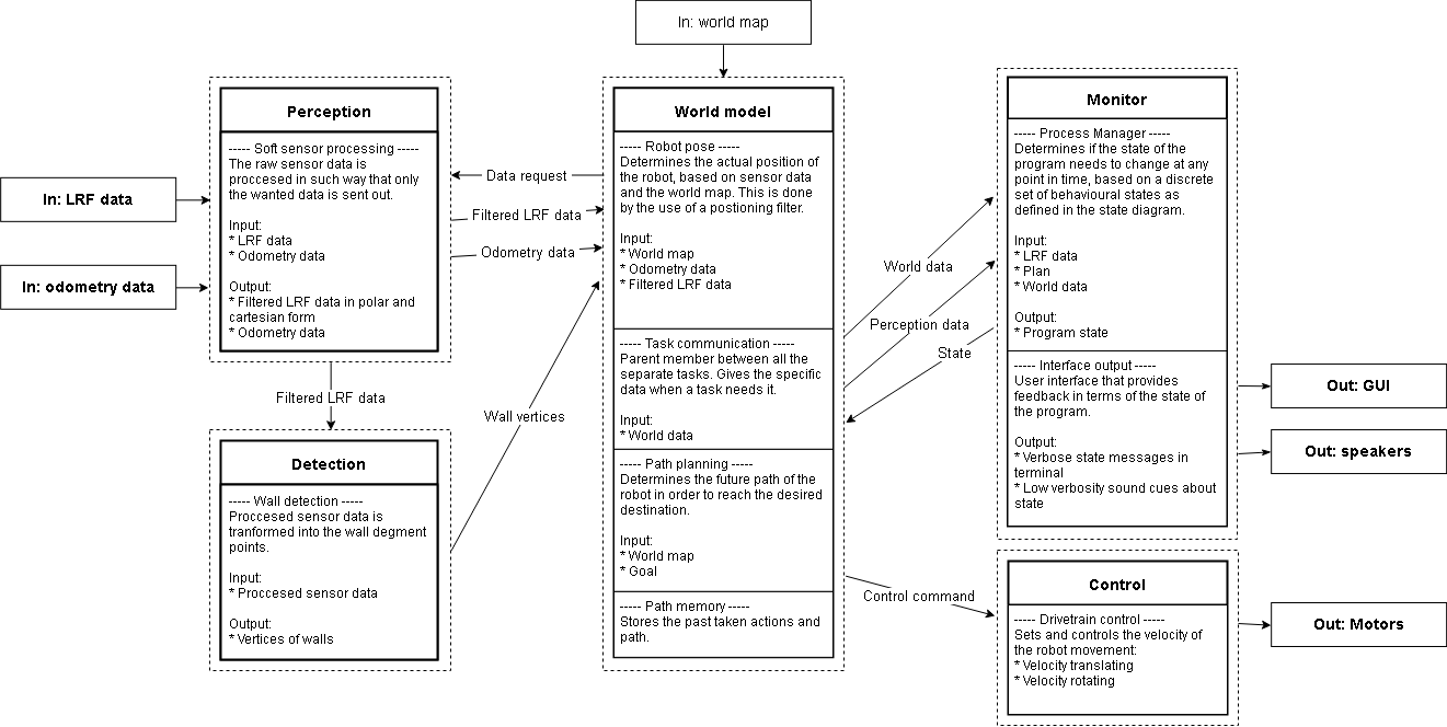
This chapter describes the various objects that the developed software is made up of. The figure below shows the final architecture diagram. This diagram describes in a nutshell what the responsibilities are of each object and how they communicate with one another. Following this diagram, each of these objects is described in detail. | |||
[[File:Concept_RobotArchitecture.png|thumb|1000px|center|Figure 5.1: system architecture of the robot software]] | |||
=== Monitor | === Monitor object === | ||
The purpose of the monitor object is to keep track of the state of the software, as well as command the state changes. This object also processes the interaction between the robot and the outside world. This includes the text-to-speech function and the user input of the cabinet order. | |||
=== | ==== State chart ==== | ||
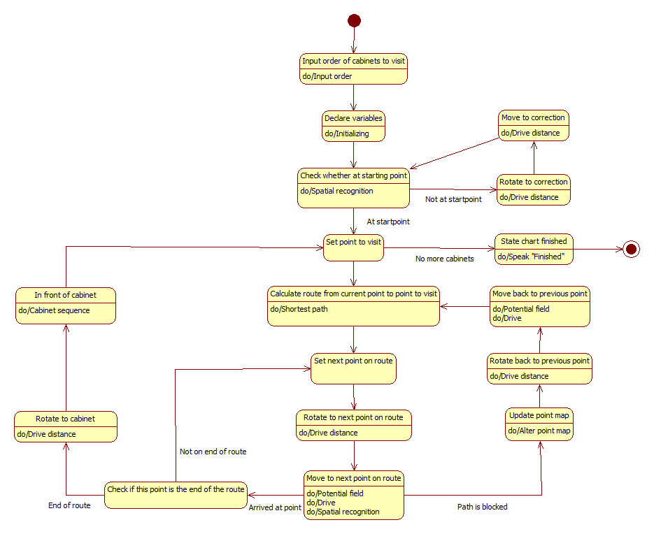
The state chart describes the steps the software needs to take in order to perform the final challenge. Each state describes an action the software needs to perform. Once this action is completed, the software will flow to the next state. At states with multiple output arrows, a decision needs to be made to which state the software will flow. This decision is always an 'if' statement in code. During the action that is performed in a state, the decision of which state the software flows to is made. Figure 5.2 shows the final state chart of the developed software. | |||
[[File:State machine final.png|800px|center|Figure 5.2: state chart|thumb]] | |||
The state chart starts at the red dot at the top. The first state is for inputting the cabinet order. That state was bypassed however, since the method of inputting the cabinet order was defined later in the assignment. The next state is for declaring variables used for the state chart. The state "Check whether at starting point" and the states to its right are for positioning the robot on the start point. These states are for localizing and driving the robot to the correct starting point. | |||
The control | The movement of the robot is split into two states. One is for rotating the robot towards the next point. The second is driving the robot towards the next point. The splitting of movement into two separate states was done to simplify the movement and to reduce the chance of collision with obstacles that are not in sight of the laser rangefinder. During every movement state, the "potential field" is turned on as to avoid collisions. This is explained in further detail in the [[#Drive control|Drive control section]]. | ||
In the "Set point to visit" state, the next cabinet that needs to be visited is selected. If there are no more cabinets left to visit, the state chart goes to the "Finished" state. The software then calculates the shortest route from its current point to the cabinet. The next states are for moving the robot from point to point until it reaches a cabinet. If a path is blocked, the software will update the point map (explained in the [[#Pathpoint route calculation|pathpoint route calculation section]]) by removing that path between the points. The software will then return to the "Set point to visit" state and recalculate the route. | |||
The state chart is implemented in the software with two functions. The first function starts the tasks that need to be performed in the function. The second function checks whether all the tasks of that state are completed. This checking happens once every "tick". A tick is a single cycle of the software. The software runs at 20 ticks per second. Once all the tasks are completed, the software will flow to the next state. Using two functions allows for other parts of the software to continue in parallel with the state chart. | |||
The | |||
=== Perception object === | |||
The purpose of the perception object is to condition the sensor data. This mainly involves filtering invalid points from the LRF measurements, such that these points cannot pollute the information that is fed into the feature detection algorithm. Such invalid points include points that are erroneously measured at the origin of the sensor, probably as a result of dust on the sensor. | |||
= | ==== LRF data conditioning ==== | ||
The | A test measurement with the robot was done to obtain raw LRF data. Analysis of this data concluded that the data contained unwanted points. These point fall into two categories. | ||
The first category is of points which are directly on the robot. These points may be caused by dirt on the LRF sensor. These points were filtered by removing al data points within a certain radius of the robot. The size of this radius was chosen to be 0.25m. | |||
The second category consists of unwanted points which were on the edges of the field of view of the LRF. The LRF measured parts of the exterior of the robot. These points were filtered by removing the first and last 10 points from the LRF data. | |||
After the data is filtered, the data is converted from polar coordinates to cartesian coordinates. This conditioned data is then accessible to the detection and world model objects. | |||
== | ==== Odometry data ==== | ||
The | The odometry data is retrieved from the robot and stored in a variable that is publicly accessible by other objects. This is done because the function that reads the data from the robot will only return the odometry data if the current data has not yet been read. Otherwise, the function returns no data. Storing the data in a publicly accessible variable allows other objects to retrieve the data as many times as they like. | ||
=== Detection object === | |||
In detection, the conditioned data of the perception block is used to create a map of the surroundings of the robot. This is then sent to the world model to localize the robot. This chapter explains how the conditioned LRF data is converted to a map of the walls and corners of the robot's surroundings. | |||
== | ==== Wall finding algorithm ==== | ||
=== | To allow PICO to navigate safely, he must know where he is in the world map and what is around him. As described earlier, PICO is equipped with a laser rangefinder that scans the environment with the help of laser beams. This data is then processed to be able to determine where all walls and objects are. There are many ways in which you can process the data into useful information. A commonly used algorithm for line extraction is the ''split and merge'' algorithm. As for fitting lines on the extracted segments, the ''RANSAC'' algorithm is used. In the case of this design, we do the following processing steps: | ||
== | # Filtering measurement data | ||
# Recognizing and splitting global segments (recognizing multiple walls or objects) | |||
# Apply the split algorithm per segment | |||
## Determine end points of segment | |||
## Determine the linear line between these end points (by = ax + c) | |||
## For each data point between these end points, determine the distance perpendicular to the line (d = abs(a*x+b*y+c)/sqrt(a^2+b^2)) | |||
## Compare the point with the longest distance with the distance limit value | |||
##* If our value falls below the limit value then there are no more segments (parts) in the global segment. | |||
##* If the value falls above the limit value, the segment is split at this point and steps 3.1 to 3.4 are performed again for the left and right parts of this point. | |||
# Lines are fitted from the segment points using the RANSAC algorithm. | |||
In figure 5.3 is a visual representation of the split principle. The original image is used from the EMC course of 2017 group 10 [http://cstwiki.wtb.tue.nl/index.php?title=Embedded_Motion_Control_2017_Group_10#Corner_detection]: | |||
The | |||
= | [[File:Split and merge resized.gif|center|alt=Split and merge procedure|Figure 5.3: split and merge procedure|frame]] | ||
The code snippet of the split and merge function can be found here [https://gitlab.tue.nl/EMC2019/group3/snippets/137]. | |||
== | As mentioned earlier, each segment is fitted to a line using the RANSAC algorithm. RANSAC (RANdom SAmple Consensus) iterates over various random selections of two points and determines the distance of every other point to the line that is constructed by these two points. If the distance of a point falls within a threshold distance, this point is considered an ''inlier''. The distance ''d'' of this inlier to the line is then compared to the threshold value ''t'' to determine how well it fits the current line iteration. This is described by the score for this point, which is calculated as ''(t - d)/t''. The sum of all scores for one line iteration is then divided by the number of points in the segment that is being evaluated. This value is the final score of the current line iteration. By iterating over various random lines among the points in the segment, the line with the highest score can be selected as being the best fit. Figure 5.4 demonstrates the basic principle of an unweighted RANSAC implementation, where only the number of inliers accounts for the score of each line. | ||
[[File:RANSAC_EMC3_2019_.gif|center|alt=Unweighted RANSAC line fitting visualisation|Figure 5.4: unweighted RANSAC line fitting visualisation|frame]] | |||
The reason that the RANSAC algorithm was selected for fitting the lines in the segments over linear fitting methods, such as least squares, is robustness. During initial testing it became clear that when the laser rangefinder scans across a dead angle, it would detect points in this area that are not actually on the map. These points should not be taken into account when fitting the line. As visualised above, these outliers are ignored by RANSAC. If a linear fitting algorithm such as least squares were to be used, these outliers would skew the actual line, resulting in inaccurate line detection. | |||
A final line correction needs to be done because the RANSAC function implementation only returns start and endpoints somewhere between the found vertices. The lines need to be fitted so that the corners and endpoints align to the real wall lines. This is simply done by determining the lines between the points and then equate the lines to each other. The final endpoints are determined by equating the point on the line where the found vertices are perpendicular to this line. | |||
The code snippet of the RANSAC function can be found here [https://gitlab.tue.nl/EMC2019/group3/snippets/136]. | |||
=== World model object === | |||
The world model is the central object in the software architecture. The purpose of the world model is to act on changes in the positioning of PICO, such as sensing where on the map PICO is, determining to which pathpoints to drive, and in which direction to drive in order to reach a pathpoint. An additional responsibility of the world model is to visualise the conditioned LRF data and the pathpoint to which PICO is driving, as well as storing snapshots of the LRF data when commanded to do so. | |||
==== Position estimation ==== | |||
Using the wall finding algorithm as described earlier, it is possible to extract the relative position in cartesian coordinates of all the visible corners. By matching these corners to the known corners from the given json file, it is possible to determine the location of PICO. This is done in one big function containing several steps. This function is constantly running in the background, and determines the absolute position of PICO, with the origin in this frame being determined as the zero point in the json file. | |||
The first step in the localization function is extracting all corner positions from the json file, as well as getting all visible corner positions from the wall finding algorithm function. Of course, these two corner positions will be given in a different frame, and as such, a conversion needs to be made from one frame to another. As such, the coordinates of the corners given from the wall finding algorithm are converted from the relative PICO frame, to the absolute frame, in order to make it similar to the json file coordinates. This may seem as a catch-22 situation, as converting these coordinates from a relative to an absolute frame requires the position and orientation of PICO, which is exactly what the output of this function will be. So the conversion is made using the last correctly found absolute coordinates and orientation of PICO. Since this function is ran with a frequency of 20 Hz, it can be assumed that the last known position and orientation will be close to the new position and orientation. | |||
The rest of the function can be divided into two steps. First, the function will determine the orientation of PICO. Next, the function will determine the position of PICO. For orientation finding, the relative to absolute conversion is made a lot of times using ‘the last known orientation-0.3’ rad to ‘last known orientation+0.3’ rad, with steps of 0.01 rad. This results in a list of sets of corner positions in absolute coordinates found using a lot of different orientations. This list of sets will be compared to corner coordinates from the json file. The next step is to see which set of corners has the least amount of variance in error when compared to the json file. This method is used because the actual absolute position of PICO will be slightly different from the absolute position used in the frame conversion, so there will always be an error. However, it can be assumed that this error should be roughly the same for all corners when the orientation is correct, and as such, the variance should be as low as possible. So all sets of corners are compared to the json file, and the set with the lowest error variance give us the best orientation estimation. | |||
With the correct orientation now known, the correct position can be determined. Two different methods are used in this function, and the average of the results of the two different methods is used as the final solution. The first method used to find the correct position is very similar to the method used for orientation, as this method creates a list of sets of corner position, were the conversion from relative to absolute is made a lot of times using ‘the last known position-1.0’ meter to ‘last known position+1.0’ meter, with steps of 0.1 meter. The steps are followed as with the orientation method, however this time the function will not look at the lowest error variance, but will simply look which set will result in the lowest error. | |||
The second method used to find the correct position goes through all found corners, looks at the found absolute position of these corners, and sees which corner coordinate from the json file is the most similar. This works as the actual absolute position of PICO cannot be too far off from the last known absolute position. When this is done for every found corner, all the errors between the found corners and their best matching json coordinate are compared. It is likely that most of these errors will be roughly the same, with perhaps some errors being totally different. These completely different errors are discarded and only the matching errors are kept. The mean of these errors will be calculated, and the resulting number will be the mismatch between the last known PICO coordinates, and the current real PICO coordinates. The new PICO coordinates can then be saved. The average of the results of this method and the previous method is than taken as the new absolute PICO position. | |||
The function will check if its new position is a realistic result. It does this by comparing it to its previous known position. Since this previous known position cannot be off by too much, it can be assumed that when there is a major difference between the new and old position, something must be wrong. If this is determined, the function will not save the new position, and instead keep the last correct position as its current position. The function will simply rerun with new sensor data to make a new estimation and hopefully, that one will be better. If the function discards the new position several times in a row, it will change some of its control numbers in the function, as to increase the range at which it will search for its correct coordinates. For example, the range of orientation finding will increase from "-0.3 to 0.3" towards "-pi to pi". This wider range numbers are also used when the function is ran for the first time, as during initialization the correct position is only known roughly, and nothing is known about orientation. | |||
The code snippet of the localisation function can be found here: [https://gitlab.tue.nl/EMC2019/group3/snippets/138]. | |||
==== Path planning ==== | |||
The method of determining the path points is done both automatically and by hand. The program will load the JSON map file when the program starts. The code will detect where all the cabinets are and what the front is of a cabinet. Each cabinet path point will exactly be placed in the middle of the virtual square area that is specified in front of the cabinet. The rest of the path points are put in by hand. A path point has three variables: the x and y coordinates and the direction. The direction only applies when the path point is in front of a cabinet. The orientation that PICO needs to have to be in front of the cabinet is specified within the direction variable. The direction will be subtracted from the real orientation of PICO and is corrected afterwards if PICO is not aligned right. Figure 5.5 shows the modified version of the hospital JSON map. | |||
[[File:JsonMapMetPathPoints.png|700px|center|thumb|Figure 5.5: modified Json map with path points]] | |||
{| class="TablePager" style="width: 230px; min-width: 240px; margin-left: 2em; float:left; color: black;" | |||
|+ '''Cabinet positioning points''' | |||
|- | |||
! scope="col" | '''Point''' | |||
! scope="col" | '''X''' | |||
! scope="col" | '''Y''' | |||
|- | |||
| 0 (cabinet 0) || 0.4 || 3.2 | |||
|- | |||
| 1 (cabinet 1) || 0.4 || 0.8 | |||
|- | |||
| 2 (cabinet 2) || 0.4 || 5.6 | |||
|- | |||
| 3 (cabinet 3) || 6.3 || 3.2 | |||
|} | |||
{| class="TablePager" style="width: 230px; min-width: 240px; margin-left: 2em; float:left; color: black;" | |||
|+ '''Path points''' | |||
|- | |||
! scope="col" | '''Point''' | |||
! scope="col" | '''X''' | |||
! scope="col" | '''Y''' | |||
|- | |||
| 4 (Start point) || 5.0 || 2.5 | |||
|- | |||
| 5 || 5.5 || 3.2 | |||
|- | |||
| 6 || 5.5 || 3.9 | |||
|- | |||
| 7 || 5.5 || 5.6 | |||
|- | |||
| 8 || 3.5 || 5.6 | |||
|- | |||
| 9 || 2.0 || 5.6 | |||
|- | |||
| 10 || 0.4 || 4.7 | |||
|- | |||
| 11 || 1.25 || 4.7 | |||
|- | |||
| 12 || 1.25 || 3.5 | |||
|- | |||
| 13 || 0.4 || 2.7 | |||
|- | |||
| 14 || 1.25 || 2.7 | |||
|- | |||
| 15 || 1.25 || 1.5 | |||
|- | |||
| 16 || 1.25 || 0.8 | |||
|- | |||
| 17 || 2.0 || 1.6 | |||
|- | |||
| 18 || 3.5 || 1.6 | |||
|- | |||
| 19 || 3.5 || 3.6 | |||
|} | |||
{| class="TablePager" style="width: 230px; min-width: 240px; margin-left: 2em; float:left; color: black;" | |||
|+ '''Path lengths (1/2)''' | |||
|- | |||
! scope="col" | '''Path''' | |||
! scope="col" | '''Length''' | |||
|- | |||
| 4->5 || 0.86 | |||
|- | |||
| 4->6 || 1.49 | |||
|- | |||
| 5->3 || 0.8 | |||
|- | |||
| 5->6 || 0.7 | |||
|- | |||
| 3->6 || 1.06 | |||
|- | |||
| 6->7 || 1.7 | |||
|- | |||
| 7->8 || 2.0 | |||
|- | |||
| 8->9 || 1.5 | |||
|- | |||
| 9->2 || 1.6 | |||
|- | |||
| 9->10 || 1.84 | |||
|- | |||
| 9->11 || 1.17 | |||
|- | |||
| 2->10 || 0.9 | |||
|- | |||
| 10->11 || 0.85 | |||
|- | |||
| 11->12 || 1.2 | |||
|} | |||
{| class="TablePager" style="width: 230px; min-width: 240px; margin-left: 2em; float:left; color: black;" | |||
|+ '''Path lengths (2/2)''' | |||
|- | |||
! scope="col" | '''Path''' | |||
! scope="col" | '''Length''' | |||
|- | |||
| 12->13 || 1.17 | |||
|- | |||
| 12->14 || 0.8 | |||
|- | |||
| 13->0 || 0.5 | |||
|- | |||
| 13->14 || 0.85 | |||
|- | |||
| 14->15 || 1.2 | |||
|- | |||
| 15->1 || 1.1 | |||
|- | |||
| 15->16 || 0.7 | |||
|- | |||
| 15->17 || 0.76 | |||
|- | |||
| 1->16 || 0.85 | |||
|- | |||
| 16->17 || 1.1 | |||
|- | |||
| 17->18 || 1.5 | |||
|- | |||
| 18->19 || 2.0 | |||
|- | |||
| 19->8 || 2.0 | |||
|} | |||
<div style="clear:both"></div> | |||
<br> | |||
In the current design of the point map, there is a possibility that some points cannot be reached because of an obstacle that is on that point. For example, if there is a obstacle on point 8, the path movement from point 7 to point 8 would be impossible to complete. This would mean that the whole left side of the map can not be accessed by the robot, since driving from point 7 to point 8 is required to get there. To solve this problem, a nunber of backup paths were added to the point map. These are paths between points that were not initially connected. These paths are defined such that the robot will only choose it if there are no other options to go to a certain point. The backup paths added are: | |||
{| class="TablePager" style="width: 100px; min-width: 110px; margin-left: 2em; float:left; color: black;" | |||
|- | |||
! scope="col" | '''Backup paths''' | |||
|- | |||
| 5->7 | |||
|- | |||
| 7->9 | |||
|- | |||
| 8->18 | |||
|} | |||
<div style="clear:both"></div> | |||
<br> | |||
==== Pathpoint route calculation ==== | |||
In the [[#Path planning|path planning section]], the method the robot uses to navigate through the hospital was explained. The robot will use a point map, where each point is connected to a different neighboring point. To get from a point to a non-neighboring point, the robot needs to travel from point to point to get there. This list of points is called the route the robots needs to travel. The pathway between points is referred to as the path. Usually, there are multiple routes from a point to another point. In this case, the shortest route is preferred, since the chance of the robot losing its position on the map is the smallest. | |||
In order to obtain the shortest route, the Dijkstra algorithm is used. This algorithm can be used to obtain the shortest path from a point to another point, given a point map and the weight of the paths between the points. This weight can be based on the distance between the points or the difficulty of the path. Dijkstra's algorithm works by creating a list of the distance from a start point to every other point. The algorithm then checks the distance to each other point, whilst updating the list of shortest distances. The algorithm also remembers the previous point from which the shortest route came. So once the shortest distance list is completed, the algorithm can backtrack the route from the end point to the starting point. | |||
Figure 5.6 illustrates how the algorithm works. Inside the points the current shortest path to the point is indicated, while the number near the path is the weight of that path. | |||
[[File:Dijkstra_EMC3_2019.gif|center|Figure 5.6: visualization Dijkstra algorithm (source: steemit.com [https://steemit.com/popularscience/@krishtopa/dijkstra-s-algorithm-of-finding-optimal-paths])|frame]] | |||
== | In the software, the point map is represented as a matrix. This matrix contains the distance from each point to every other point. Such an example matrix is shown below. In this matrix, point d[1,n] is the weight from point 1 to point n. Value d[n,1] will be the same, as this is the distance from point n to point 1. If, for example, point 1 and point two would not be connected, the value in the matrix would be d[1,2] = d[2,1] = 0. | ||
The weight of the path is represented by a number greater than 0. The greater the number, the more difficult the path. The diagonal of the matrix contains the distances from each point to itself. Therefore, this value should always be zero (d[n,n] = 0). | |||
[[File:Pointmap_matrix.PNG|200px|center|Point map matrix]] | |||
= | Based on the mentioned properties of the point matrix, it can be concluded that this matrix should always be symmetric and always have only zeroes in the diagonal. These properties can be used when to check whether the inputted map is free of errors. Furthermore, editing the point matrix is simple. If a path between point n and point m needs to be added or removed, all that needs to be done is change the values such that d[m,n] = d[n,m] = w, where w is the new weight of that path. If a path needs to be removed, w should be equal to 0. | ||
== | ==== Drive target calculation ==== | ||
Now that both the absolute position of PICO and that of the next pathpoint are known on the map, the robot needs to know in which direction to drive. That means that the location of the pathpoint that PICO should drive to, needs to be transformed to the coordinate space of PICO. This way it can be figured out in which relative direction PICO should drive and how much PICO should rotate before driving. The results of the calculations is visualised in figure 5.7. | |||
[[File: | [[File:Coordinate_transform_EMC3_2019.png|center|Figure 5.7: diagram of coordinate space transformation parameters|500px|thumb]] | ||
The first step is to determine the difference vector [[File:V_delta_EMC3_2019.png|frameless|upright=0.1]] between the position of the pathpoint [[File:V_point_EMC3_2019.png|frameless|upright=0.2]] and the position of PICO [[File:V_pico_EMC3_2019.png|frameless|upright=0.2]]. This is done by a simple subtraction: | |||
[[File:V_delta_calc_EMC3_2019.png|center|frameless|upright=0.75]] | |||
== | Then the coordinate space matrix of PICO [[File:S_pico_EMC3_2019.png|frameless|upright=0.2]] needs to be determined in order to create the transition matrix. This is done by using the absolute rotation of PICO [[File:Th_pico_EMC3_2019.png|frameless|upright=0.2]] in order to calculate the unit vector components of the x- and y-axes of the PICO coordinate space within the absolute coordinate space. | ||
[[File: | [[File:S_pico_calc_EMC3_2019.png|center|frameless|upright=1.5]] | ||
Then the relative position vector of the pathpoint in PICO's coordinate space [[File:V_point_pico_EMC3_2019.png|frameless|upright=0.2]] can be calculated by multiplying the inverse of the PICO space matrix with the difference vector: | |||
[[File:V_point_pico_calc_EMC3_2019.png|center|frameless|upright=0.75]] | |||
With the relative coordinates known of the next pathpoint, PICO knows how far to turn in a certain direction before driving and where to aim for when avoiding obstacles. This requires the relative position of the targeted pathpoint to be recalculated every tick, so the driving code can correct for changes in direction in real time. | |||
==== Visualisation ==== | |||
Several visualisation functions were made for the sake of debugging the trajectory of PICO. These functions are built upon the OpenCV framework and are meant to streamline the process of drawing the LRF data, the detected walls, targeted pathpoints, and PICO itself. These functions require a Mat object as an input (pass by reference) and then they draw their shapes on there. This way, all the data can be passed into these functions using world units without the need for converting everything to pixel positions within the image. | |||
By stacking all the mentioned functions on a single Mat object, the main visualiser of the program was created. A gif of the visualiser in a simulated environment is displayed in figure 5.8. The blue point represents the active target of PICO at any given time. The walls are drawn in white on top of the green LRF data. | |||
[[File:Visualisation_EMC3_2019.gif|center|Figure 5.8: visualisation of the final software|frame]] | |||
Lastly, a function was made to take snapshots of the LRF data when PICO arrives at a cabinet. These snapshots are written to the "Snapshots" folder in the project directory, and contain information in the filename of the snapshot number and the cabinet number. This function makes use of the function that scatters the LRF data on a Mat object, that was mentioned earlier. The function to draw PICO on the image is also used. The resulting Mat object is then written to a .png file using the OpenCV function "imwrite." An example snapshot that was made in the simulation environment is shown in figure 5.9. | |||
[[File:Snapshot_simulation_EMC3_2019.png|center|Figure 5.9: snapshot of cabinet 0 taken during simulation: "Snapshot 2 cabinet 0.png"|frame]] | |||
=== Control object === | |||
The control object contains the actuator control, called drive control. This object provides output to the actuators based on inputs from the world model. | |||
==== Drive control ==== | |||
The actuators are controlled such that the movement of the robot is fluent. This is achieved by implementing an S-curve for any velocity change. The S-curve implementation was chosen to limit jerk in the robot's movement and thus preventing slip. The reduction of slip in the motion of PICO increases the accuracy of its movement on top of the fluency. The S-curve is implemented in two different functions; the function 'Drive' accelerates and decelerates smoothly to a certain speed or rotation in any direction. The second function 'Drive distance' accurately accelerates and decelerates over a fixed distance or rotation. General information on S-curves can be found via the link under [[Useful information|useful information]]. | |||
Drive control has been further incorporated in a function that uses a potential field. This function prevents the robot from bumping into objects in a fluent manner. See figure 5.10 for a visual representation of an example potential field. The leftmost image shows the attraction field to the goal, the middle image shows the repulsion from obstacles and the rightmost image shows the combination of the two. Any wall or object is taken into account for this function. | |||
[[File:Potential_field.png|1000px|center|thumb|Figure 5.10: potential field principle (source: [https://www.ais.uni-bonn.de/papers/ISPRS_nieuw_schad_beh.pdf])]] | |||
However, the implementation used for PICO does not use an attraction field, only repulsion from obstacles. The potential field vector is calculated in real-time, as the robot is expected to run into dynamic obstacles in the final challenge. This also takes the imperfections in the physical environment into account. The way the potential field is obtained is visualised in figure 5.11. | |||
[[File:PotentialFieldCalculationSchematic_EMC3_2019.png|1000px|center|thumb|Figure 5.11: practical examples of the behaviour of the potential field vector]] | |||
The first image shows how the robot is far away enough from any walls or obstacles, and thus the potential field vector is zero, causing the robot to keep its (straight) trajectory. In the second image, the robot is driving through a narrow corridor. As a result of the symmetry of the environment, the potential field component vectors cancel each other out, causing the potential field sum vector to be zero. Once again, the robot keeps its trajectory. In the third image however, the robot is closer to the left wall, causing the left potential field component vectors to outweigh the right ones. As such, the potential field sum vector points to the right, causing the robot to drive towards the middle of the corridor, until the sum vector reaches its steady state value when the robot is in the middle again. The fourth image depicts a situation where an obstacle, such a random box or a walking person, enters the avoidance region around the robot. Once again, the potential field sum vector points away from the obstacle, causing the robot to drive around the obstacle as depicted by the dotted line. | |||
The | |||
Although the potential field prevents collision with obstacles, it also pushes PICO off course. To make sure that PICO still reaches its goal, an orientation correction was implemented. This function uses the position data to calculate PICO's orientation relative to its current goal. If this orientation differs from the desired orientation, namely that PICO looks directly at its goal, the difference in angle is corrected. | |||
= Testing = | |||
This chapter describes the most important tests and test results during this project. | |||
==Test Goals== | |||
Several tests were executed during the course of the project, each with a different goal. The most important goals are summarised below: | |||
* Test the laser rangefinder and the encoders. | |||
* Determine the static friction in the actuators for the x- and y-direction, and the rotation. | |||
* Collect laser data for the spatial recognition functions. | |||
* Test the drive control functionality, consisting of the S-curve implementation and the potential field. | |||
* Test the full system on the example map. | |||
==Results== | |||
The results from each test are described in separate parts. | |||
=== | ===Laser rangefinder & motor encoders=== | ||
The range of the laser range finder according to the simulation is 10cm to 10m, the angle is +114.6 to -114.6 degrees as measured from the front of the robot. This angle is measured in 1000 parts, per an amount of time that can be determined by the user. However, the actual range is much larger. During the test, laserdata appeared within the 10cm radius of the robot. This data produced false positives and had to be filtered out. The maximum range of the range finder was actually larger than 10 meters, but this does not limit the functionality of the robot. The other properties of the laser range finder were accurate. | |||
The values supplied by the encoders are automatically converted to distance in the ''x''- and ''y''-direction in meters and a rotation ''a'' in radians. Due to the three wheel base orientation of the actuators, the ''x''- and ''y''-direction movement estimation are less accurate than that of the the rotation. | |||
=== | ===Static friction=== | ||
The | The actuators have a significant amount of static friction. The exact amount of friction in both translational and the rotational direction was difficult to determine. An attempt was made by slightly increasing the input velocity for a certain direction until the robot began to move. This differed for each test, so the average was taken as a final value for the drive control code. It is important to note that the friction was significantly less for the rotational direction than the translational directions. The ''y''-direction had the most friction and also had the urge to rotate instead of moving in a straight line, especially at low velocities. | ||
=== | ===Laser data=== | ||
Due to the limited testing moments, some laserdata was recorded in different situations. This data could be used to test the spatial recognition functions outside the testing moments. Data was recorded in different orientations and also during movement of the robot. | |||
=== | ===Drive control=== | ||
This test was executed to determine if the smoothness and accuracy of the drive control functions were sufficient or if the acceleration would have to be reduced. Both the smoothness and the accuracy were satisfactory, especially for the rotational movement. | |||
The potential field was also tested by walking towards the robot when it was driving forward. It successfully evaded the person in all directions while continuously driving forward. | |||
The | ===Full system test=== | ||
The full system test was executed on the provided example map. However, during this test, no dynamic or static obstacles were present that were not on the map. PICO was able to find the cabinets in the correct order from different starting positions and orientations, but the limited space between the two cabinets provided some difficulties. Since PICO is supposed to return to its previous navigation point if the orientation in front of a cabinet failed, and this point was in between the two cabinets, this caused some issues. However, in the Hospital challenge map, no two navigation points were placed as close together as in the example map, which should circumvent this issue. | |||
= Conclusion & Recommendations = | |||
In conclusion, the software implementation of the design described in this Wiki is capable of fulfilling the basic functionality of the hospital challenge. That is, if the hospital environment only contains the necessary wall geometry and the cabinets. The addition of static and dynamic obstacles proved difficult to handle by the position estimation code, and ultimately led to the robot miscalculating the orientation at the end of the hospital challenge. | |||
It is recommended to dedicate the last week before the challenge to testing all the integrated code. This is because the software described in this Wiki was only ever fully implemented during the challenge itself, and the execution proved that the robot was still susceptible to disturbances in the environment in the form of dynamic obstacles. This could have been prevented by fine-tuning several variables in the code. Secondly, it is recommended to dedicate the most time and resources to the position estimation, as this is a crucial element that is relied upon for decision-making in the state machine and calculating the movement trajectory. The potential field implementation, however, proved very robust and simple to implement. It is therefore recommended to other groups to implement this to avoid collision with static and dynamic obstacles. | |||
As a group, we take pride in the fact that we were the only group that managed to land in the top 3 of best performing challenge executions at the end of both the escape room challenge and the hospital challenge. | |||
= | [[File:Pico3th.png|thumb|center|400px|alt=Pico3th|Proud to be in 3rd place (source: [http://cstwiki.wtb.tue.nl/index.php?title=Embedded_Motion_Control_2017_Group_10#The_day_of_the_challenge])]] | ||
= | = Appendices = | ||
This chapter contains some documents that are of minor importance to the project. | |||
== | == Useful information == | ||
[https://www.robotshop.com/media/files/pdf/gostai-jazz-information-sheet.pdf Robot specs document] | |||
[http://www.et.byu.edu/~ered/ME537/Notes/Ch5.pdf S-curve equations] | |||
[[:Media:4SC020_Design_Document_2019_Group_3.pdf|PDF of initial Design Document]] | |||
== Minutes == | |||
This document contains the minutes of all meetings: | |||
[[:Media:Minutes_Group_3.pdf|Minutes]] | |||
Latest revision as of 16:22, 21 June 2019
Group members
| Collin Bouwens | 1392794 | |
| Yves Elmensdorp | 1393944 | |
| Kevin Jebbink | 0817997 | |
| Mike Mostard | 1387332 | |
| Job van der Velde | 0855969 |
Introduction
This wiki page describes the approach and process of group 3 concerning the Escape room challenge and the Hospital challenge with the PICO robot. The PICO robot is a telepresence robot that is capable of driving around while monitoring its environment. In the Escape Room Competition, the robot is placed somewhere inside a rectangular room with unknown dimensions with one doorway that leads to the finish line. Once the robot crosses the finish line without bumping into walls, the assignment is completed. The Hospital challenge involves a dynamic hospital-like environment, where the robot is assigned to approach a number of cabinets based on a known map, while avoiding obstacles.
The wiki is subdivided in the following parts: Firstly, the approach for the Escape room challenge is explained and evaluated. The second topic is the approach and evaluation of the Hospital challenge. This is followed by a full description of the system architecture used to perform the Hospital challenge. After the system architecture, the most important tests and test results are explained. Lastly, a conclusion and recommendation is provided.
Escape room challenge
This chapter summarizes the approach for the escape room challenge and offers some reflection on the execution of the challenge. Figure 3.1 shows a small clip of our execution of the robot during the escape room challenge.
Approach
The state chart in figure 3.2 depicts the wall following program that the robot is to execute during the escape room challenge. In a nutshell: the robot drives forward until a wall is detected, lines up with said wall to the right, and starts following it by forcing itself to stay between a minimum and a maximum distance to the wall. When something is detected in front, it is assumed that the next wall to follow is found, and thus the robot should rotate 90 degrees counterclockwise so it can start following the next wall. When a gap is detected to the right of the robot, it is assumed that the exit corridor has been found, and thus the robot should turn into the exit. Then the robot keeps following the right wall in the corridor until, once again, a gap is detected to the right of the robot. At this point, the robot should have crossed the finish line.

Reflection
Due to a lack of time and more resources being put into the final challenge, the code for the escape room challenge had to be simplified. The original plan was to have the robot scan the environment, identify the exit, and when identified, drive towards the exit and drive to the finish line. In case the robot could not identify the exit, the robot would start following the wall instead, as a robust backup plan. The testing session before the challenge proved to be too short, and only the wall follower could be tested. Therefore, only the wall follower program was executed during the challenge.
As a precaution to not bump into the walls, we reduced the speed of the robot and increased the distance the robot would keep to the wall by modifying the config file in the software. Although our program did succeed the challenge, we were the slowest performing group as a result of the named modifications to the configuration. We felt however that these modifications were worth the slowdown and proved the robustness of the simple approach our software took.
Hospital Competition
This chapter summarizes the approach for the hospital challenge and offers some reflection on the execution of the challenge.
Approach
The general approach to the challenge is to create a point map of the map of the hospital. Figure 4.1 shows such a point map:
A point is placed on different locations on the map. These locations are: at cabinets, on junctions, in front of doorways and in rooms. In the placement of these points, it is important that each point can be approached from a different point in a straight line. The goal of these points is that the robot can navigate from one side of the hospital to the other by driving from point to point. The points that the robot can drive to in a straight line from a point are its neighboring points.
The original plan was to define the placement of each point by the distance and direction to its neighboring points and its surrounding spatial features. However, due to a lack of development time, it was decided to simply define absolute coordinates for each point. When the robot is on a point (A) and wants to drive to a different point (B), the robot can use the distance and direction to from A to B to drive to where B approximately is. Then, using the spatial features surrounding point B, the robot can more accurately determine its location compared to B and drive to B. For the path between points, it can be defined whether this path is through a doorway or hallway, or whether it is through a room. This can help in how the robot trajectory should be controlled during the driving from point to point.
If the robots needs to drive from a starting point to an endpoint which is not neighbouring, the software will create a route to that point. This route is a list of points to which the robot needs to drive to get to the endpoint. To make sure the route is as efficient as possible, an algorithm is used which calculates the shortest route. The algorithm that is used is called "Dijkstra'a algorithm". A similar algorithm is also used in car navigation systems to obtain the shortest route.
Reflection
All sections of the final PICO program were operational and working in time for the final challenge. These together create a functioning solving plan as we had envisioned. This final program was tested in different simulation environments matching the final challenge. In the first simulation, a copy of the map of the final challenge was used, but without any static or dynamic objects, as wel as no closed doors. In this simulation everything was working very well, however, there was a chance that PICO could lose its position when it was doing its cabinet procedure. At the time of testing, the robot gets very close to the cabinet, and as a result, it sees a lot less of the room, which can cause the position estimation to act up. Other simulation tests used the same maps, but with added static obstacles and closed doors. In these tests it was noticed that the robot seemed to have more problems. The problems mostly arise from the robot losing its position due to matching the corners of static objects with points on the map. Doors also gave the added problem that a closed door may obscure corners that should actually be there. In general, we can determine that if the amount of visible corners gets too low, or there are too many wrong corners, the robot will lose its position. At that moment the position estimation code will try to fix this. This will work most of the time, but sometimes it will not be able to find the correct position again, or it will fix it in a completely wrong way. When that happens, there is no way to fix it anymore. By running these simulation tests a lot of time, we estimated that we had a 40% chance of completing the final challenge.
During the final challenge, the robot had to visit the cabinets in order 0, 1, 3. The door was closed between 0 and 1, so the robot would have to find a alternative route between 0 and 1. Furthermore, there were some static obstacles, especially a big one in the hallway and in room 1, but less than we had anticipated. There was also one dynamic object, with which we had not run any tests beforehand, so we were not sure how the robot would react to that. Each group had two runs it could do.
The first leg of the challenge went very well. The robot first had to determine its orientation, which it was able to do excellently during both runs. Figure 4.2 shows how PICO was able to determine its original orientation and how it corrects for this.
It will then go from the starting area to the hallway, from which it will go to room 2 and then end in room 0, as this route is the shortest route. Indeed, this is exactly what the robot did, as can be seen in figure 4.3. It went from waypoint to waypoint on the map, as we had defined it. It did so in a smooth manner, indicating that there were no issues with localization at this moment.
When it arrived in room 0, it drove up to the correct side of cabinet 0, turned in the correct way, and drove up to the cabinet. This is shown in figure 4.4. In the first run, it did this in a correct manner, but in the second run, it did not drive close enough to the cabinet, and the jury was not sure if cabinet was correctly reached.
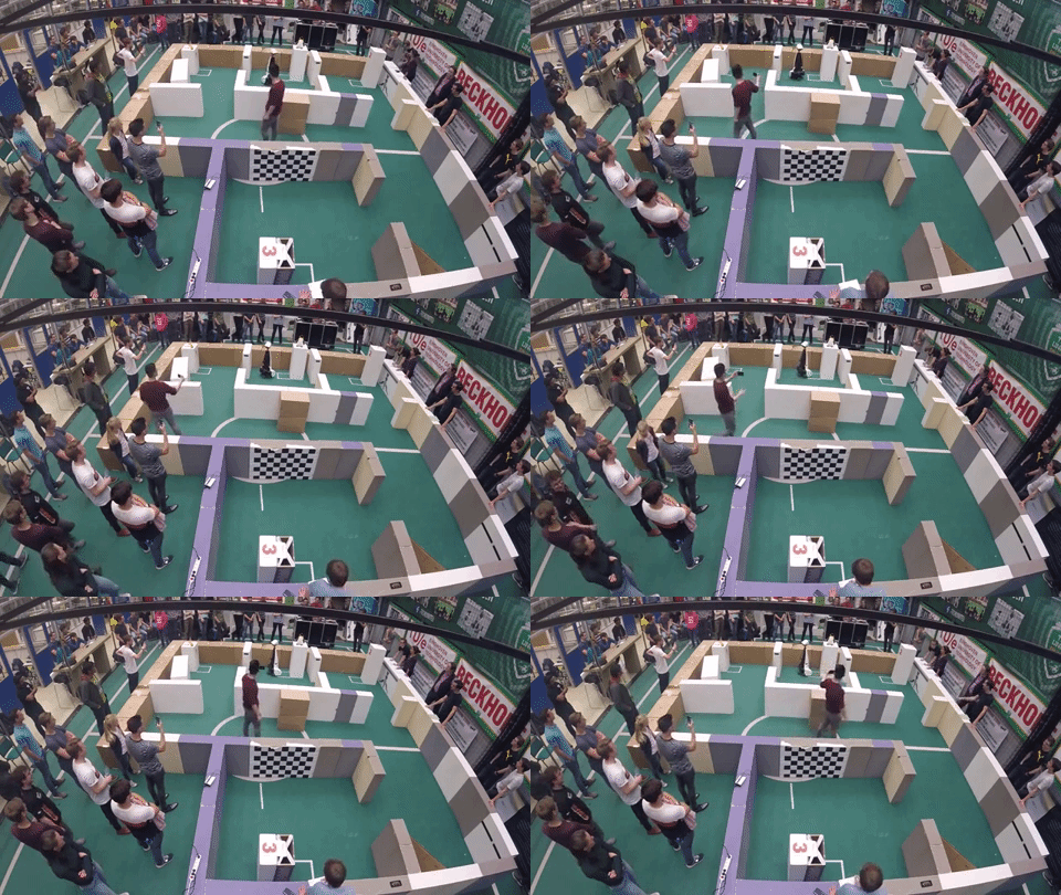
Next, the robot had to go to cabinet 1. Normally the fastest route would be going from room 0 to room 1, but the door between them was closed. So the robot had to drive to the door to notice this. At this moment the first problems with localization arose, in both runs. As we had noticed in the tests, the robot had difficulty estimating its position when it is located very closely to the cabinet, and while the robot was moving from the cabinet to the door, it first went the wrong way, towards the wall. It did this in both runs. In run 1, it merely scraped the wall, but in test 2, it bumped quite hard into the wall. The potential field should have stopped the robot from bumping into the wall, even though it lost its position, but this was not able to prevent it. In both runs however, the robot was able to fix its position eventually.
It then drove up to the door, waited for a while, and then correctly determined that this door was closed. It was able to do this correctly in run 1, as displayed in figure 4.5.
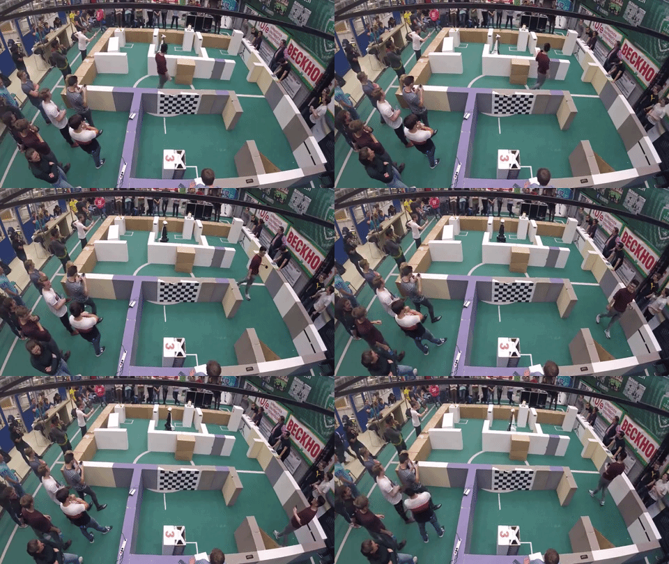
In run 2 the robot again lost its position at this instant, and again drove straight into the wall, knocking the wall completely out of place. This meant the end for the second run. In the first run however, it was able to keep its position, and go to the hallway again. This is shown in figure 4.6.
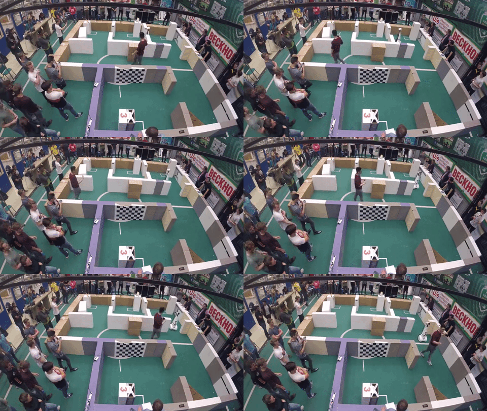
In the hallway it had to go from one end to the other, with one big obstacle in the way, and a person walking around the hallway. This proved to be too much for PICO, as it again seemed to lose its position. It tried to fix this, but it was not able to localize correctly anymore, which meant the end of the first run. This attempt is shown in figure 4.7.
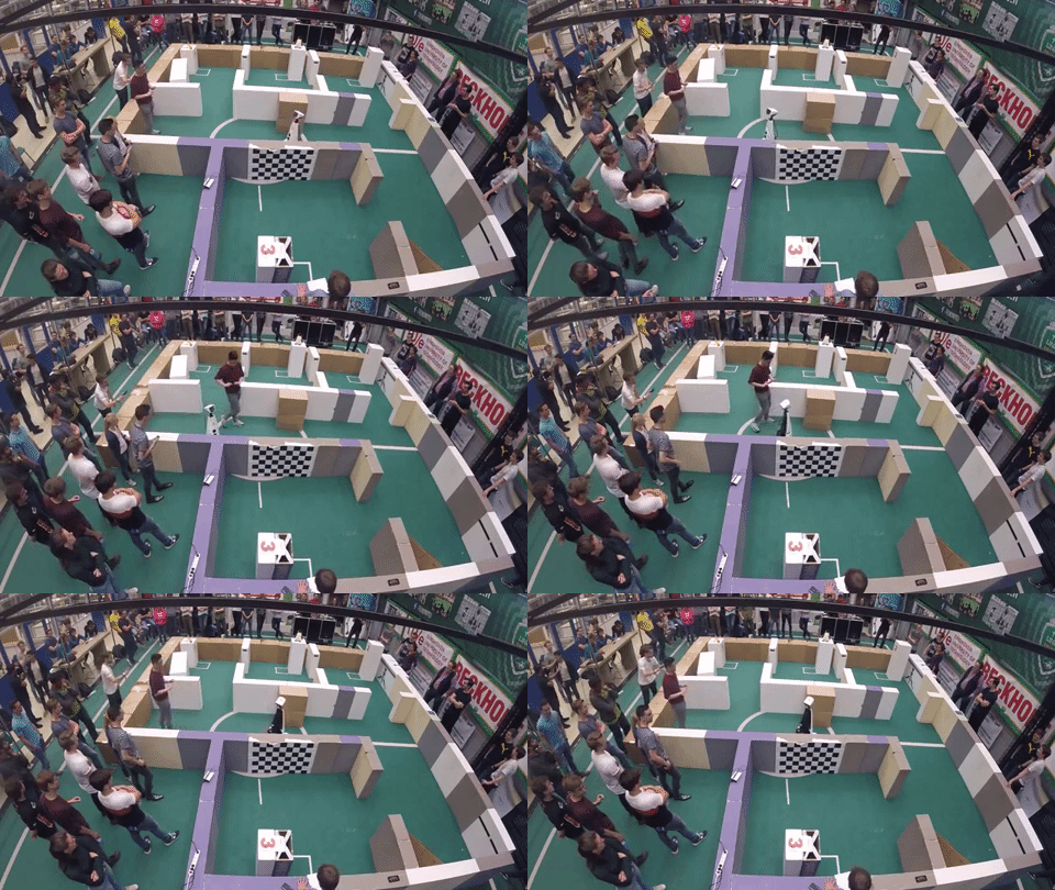
In both runs, the robot was able to find the first cabinet, complete the procedure there, and was able to determine another route because of a closed door. However, going from cabinet 0 to cabinet 1 proved too difficult for the robot, which mainly has to do with localization issues. This was something that we had anticipated, but we are very happy that PICO was able to show a correct first part in both runs. Localization seemed to be the biggest and most difficult issue to tackle, so more time could have been spent on this aspect of the program.
One detail that was discovered after the challenge though, is that the snapshots that were supposed to be taken during the cabinet procedure were nowhere to be found in the project directory on PICO. That is a problem, as it was a requirement of the challenge to take snapshots of the LRF data during the cabinet procedure. A cause for this could be that the folder that the files were to be written to did not yet exist on the robot. An example snapshot that was taken during simulations can be found in the Visualisation section.
System Design
This chapter describes the final system design for the hospital challenge. The system design is based on the original Design Document that can be found under Useful Documents.
Components
The PICO robot is a modified version of the Jazz robot, which is originally developed by Gostai, now part of Aldebaran. The key components of the robot that are relevant to this project are the drivetrain and the laser rangefinder. The drivetrain is holonomic, as it consists of three omni-wheels that allow the robot to translate in any direction without necessarily rotating. This adds the benefit of scanning the environment in a fixed orientation, while moving in any direction. The software framework allows the forward and sideways velocity to be set, as well as the horizontal angular velocity. The framework also approximates the relative position and angle from the starting position.
The laser rangefinder is a spatial measurement device that is capable of measuring the horizontal distance to any object within a fixed field of view. The software framework measures a finite number of equally distributed angles within the field of view and notifies when new measurement data is available. Using this data, walls and obstacles in the environment of the robot can be detected.
Lastly, the robot is fitted with loudspeakers and a WiFi connection according to the data sheet of the Jazz robot. This can be useful for interfacing during operation, as described in the 'Interfaces' section. Whether the PICO robot actually has these speakers and the WiFi connectivity remains to be determined.
Requirements
Different requirement sets have been made for the Escape Room Competition and the Final Competition. The requirements are based on the course descriptions of the competitions and the personal ambitions of the project members. The final software is finished once all the requirements are met.
The requirements for the Escape Room Competition are as follows:
- The entire software runs on one executable on the robot.
- The robot is to autonomously drive itself out of the escape room.
- The robot may not 'bump' into walls, where 'bumping' is judged by the tutors during the competition.
- The robot may not stand still for more than 30 seconds.
- The robot has five minutes to get out of the escape room.
- The software will communicate when it changes its state, why it changes its state and to what state it changes.
The requirements for the Final Competition are as follows:
- The entire software runs on one executable on the robot.
- The robot is to autonomously drive itself around in the dynamic hospital.
- The robot may not 'bump' into objects, where 'bumping' is judged by the tutors during the competition.
- The robot may not stand still for more than 30 seconds.
- The robot can visit a variable number of cabinets in the hospital.
- The software will communicate when it changes its state, why it changes its state and to what state it changes.
- The robot navigates based on a provided map of the hospital and data obtained by the laser rangefinder and the odometry data.
Functions
A list of functions the robot needs to fulfil has been made. Some of these functions are for both competitions, while some are for either the Escape Room or Final Competition. These functions are:
- In general:
- Recognising spatial features;
- Preventing collision;
- Conditioning the odometry data;
- Conditioning the rangefinder data;
- Communicating the state of the software.
- For the Escape Room Competition:
- Following walls;
- Detecting the end of the finish corridor.
- For the Final Competition:
- Moving to points on the map;
- Calculating current position on the map;
- Planning the trajectory to a point on the map;
- Approaching a cabinet based on its location on the map.
The key function in this project is recognising spatial features. The point of this function is to analyse the rangefinder data in order to detect walls, convex or concave corners, dead spots in the field of view, and gaps in the wall that could be a doorway. This plays a key role during the Escape Room Competition in order to detect the corridor with the finish line in it, and therefore has a priority during the realisation of the software. For this function to work reliably, it is essential that the rangefinder data is analysed for noise during the initial tests. If there is a significant amount of noise, the rangefinder data needs to be conditioned before it is fed into the spatial feature recognition function. As a safety measure, it is important to constantly monitor the spatial features in order to prevent collisions with unexpected obstacles.
Lastly, the trajectory planning function plays a major role during the Final Competition, as this determines the route that the robot needs to follow in order to get to a specified cabinet. This function needs to take obstacles into account, in case the preferred route is obstructed. This is possible, as the documentation about the Final Competition show a map in which multiple routes lead to a certain cabinet. One of these routes can be blocked, in which case the robot needs to calculate a different route.
Specifications
The specifications describe important dimensions and limitations of the hardware components of the robot that will be used during the competitions. For each component, the specifications of that components will be given, with a source of where this specification comes from.
The drivetrain of the robot can move the robot in the x and y directions and rotate the robot in the z direction. The maximum speed of the robot is limited to ±0.5 m/s translation and ±1.2 rad/s rotation. These values are from the Embedded Motion Control Wiki page. The centre of rotation of the drivetrain needs to be known in order to predict the translation of the robot after a rotation. This will be determined with a measurement.
The dimensions of the footprint of the robot need to be known in order to move the robot through corridors and doorways without collision. The footprint is 41 cm wide and 35 cm deep, according to the Jazz robot datasheet. A measurement will be made to check these dimensions.
The laser rangefinder will be used to detect and measure the distance to objects in the vicinity of the robot. The measurement distance range of the sensor is from 0.1 m to 10.0 m with a field of view of 229.2°. The range of the sensor is divided into 1000 parts. These values are determined with the PICO simulator and need to be verified with measurements on the real robot.
Interfaces
The interfacing of the robot determines how the project members interact with the robot in order to set it up for the competitions. It also plays a role during operation, in the way that it interacts with the spectators of the competitions. On the development level there is an Ethernet connection available to the robot. This allows a computer to be hooked up to the robot in order to download the latest version of the software using git, by connecting to the Gitlab repository of the project group. This involves using the git pull command, which downloads all the content from the repository, including the executable that contains the robot software.
On the operation level it is important for the robot to communicate the status of the software. This is useful for debugging the software, as well as clarifying the behaviour during the competitions. This can be made possible with the loudspeaker, by recording voice lines that explain what the robot currently senses and what the next step is that it will perform. Not only is this functionally important, but it can also add a human touch to the behaviour of the robot. In case that the PICO robot has been altered to not have loudspeakers, it needs to be determined during testing if the WiFi interface can be utilised in order to print messages in a terminal on a computer that is connected to the robot.
System architecture
This chapter describes the various objects that the developed software is made up of. The figure below shows the final architecture diagram. This diagram describes in a nutshell what the responsibilities are of each object and how they communicate with one another. Following this diagram, each of these objects is described in detail.
Monitor object
The purpose of the monitor object is to keep track of the state of the software, as well as command the state changes. This object also processes the interaction between the robot and the outside world. This includes the text-to-speech function and the user input of the cabinet order.
State chart
The state chart describes the steps the software needs to take in order to perform the final challenge. Each state describes an action the software needs to perform. Once this action is completed, the software will flow to the next state. At states with multiple output arrows, a decision needs to be made to which state the software will flow. This decision is always an 'if' statement in code. During the action that is performed in a state, the decision of which state the software flows to is made. Figure 5.2 shows the final state chart of the developed software.
The state chart starts at the red dot at the top. The first state is for inputting the cabinet order. That state was bypassed however, since the method of inputting the cabinet order was defined later in the assignment. The next state is for declaring variables used for the state chart. The state "Check whether at starting point" and the states to its right are for positioning the robot on the start point. These states are for localizing and driving the robot to the correct starting point. The movement of the robot is split into two states. One is for rotating the robot towards the next point. The second is driving the robot towards the next point. The splitting of movement into two separate states was done to simplify the movement and to reduce the chance of collision with obstacles that are not in sight of the laser rangefinder. During every movement state, the "potential field" is turned on as to avoid collisions. This is explained in further detail in the Drive control section. In the "Set point to visit" state, the next cabinet that needs to be visited is selected. If there are no more cabinets left to visit, the state chart goes to the "Finished" state. The software then calculates the shortest route from its current point to the cabinet. The next states are for moving the robot from point to point until it reaches a cabinet. If a path is blocked, the software will update the point map (explained in the pathpoint route calculation section) by removing that path between the points. The software will then return to the "Set point to visit" state and recalculate the route.
The state chart is implemented in the software with two functions. The first function starts the tasks that need to be performed in the function. The second function checks whether all the tasks of that state are completed. This checking happens once every "tick". A tick is a single cycle of the software. The software runs at 20 ticks per second. Once all the tasks are completed, the software will flow to the next state. Using two functions allows for other parts of the software to continue in parallel with the state chart.
Perception object
The purpose of the perception object is to condition the sensor data. This mainly involves filtering invalid points from the LRF measurements, such that these points cannot pollute the information that is fed into the feature detection algorithm. Such invalid points include points that are erroneously measured at the origin of the sensor, probably as a result of dust on the sensor.
LRF data conditioning
A test measurement with the robot was done to obtain raw LRF data. Analysis of this data concluded that the data contained unwanted points. These point fall into two categories. The first category is of points which are directly on the robot. These points may be caused by dirt on the LRF sensor. These points were filtered by removing al data points within a certain radius of the robot. The size of this radius was chosen to be 0.25m. The second category consists of unwanted points which were on the edges of the field of view of the LRF. The LRF measured parts of the exterior of the robot. These points were filtered by removing the first and last 10 points from the LRF data. After the data is filtered, the data is converted from polar coordinates to cartesian coordinates. This conditioned data is then accessible to the detection and world model objects.
Odometry data
The odometry data is retrieved from the robot and stored in a variable that is publicly accessible by other objects. This is done because the function that reads the data from the robot will only return the odometry data if the current data has not yet been read. Otherwise, the function returns no data. Storing the data in a publicly accessible variable allows other objects to retrieve the data as many times as they like.
Detection object
In detection, the conditioned data of the perception block is used to create a map of the surroundings of the robot. This is then sent to the world model to localize the robot. This chapter explains how the conditioned LRF data is converted to a map of the walls and corners of the robot's surroundings.
Wall finding algorithm
To allow PICO to navigate safely, he must know where he is in the world map and what is around him. As described earlier, PICO is equipped with a laser rangefinder that scans the environment with the help of laser beams. This data is then processed to be able to determine where all walls and objects are. There are many ways in which you can process the data into useful information. A commonly used algorithm for line extraction is the split and merge algorithm. As for fitting lines on the extracted segments, the RANSAC algorithm is used. In the case of this design, we do the following processing steps:
- Filtering measurement data
- Recognizing and splitting global segments (recognizing multiple walls or objects)
- Apply the split algorithm per segment
- Determine end points of segment
- Determine the linear line between these end points (by = ax + c)
- For each data point between these end points, determine the distance perpendicular to the line (d = abs(a*x+b*y+c)/sqrt(a^2+b^2))
- Compare the point with the longest distance with the distance limit value
- If our value falls below the limit value then there are no more segments (parts) in the global segment.
- If the value falls above the limit value, the segment is split at this point and steps 3.1 to 3.4 are performed again for the left and right parts of this point.
- Lines are fitted from the segment points using the RANSAC algorithm.
In figure 5.3 is a visual representation of the split principle. The original image is used from the EMC course of 2017 group 10 [4]:
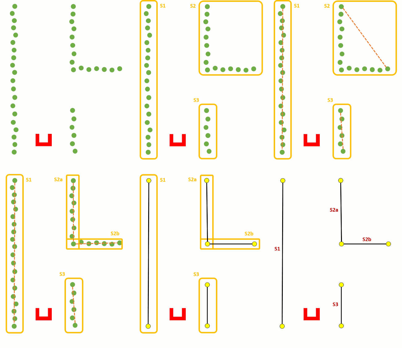
The code snippet of the split and merge function can be found here [5].
As mentioned earlier, each segment is fitted to a line using the RANSAC algorithm. RANSAC (RANdom SAmple Consensus) iterates over various random selections of two points and determines the distance of every other point to the line that is constructed by these two points. If the distance of a point falls within a threshold distance, this point is considered an inlier. The distance d of this inlier to the line is then compared to the threshold value t to determine how well it fits the current line iteration. This is described by the score for this point, which is calculated as (t - d)/t. The sum of all scores for one line iteration is then divided by the number of points in the segment that is being evaluated. This value is the final score of the current line iteration. By iterating over various random lines among the points in the segment, the line with the highest score can be selected as being the best fit. Figure 5.4 demonstrates the basic principle of an unweighted RANSAC implementation, where only the number of inliers accounts for the score of each line.
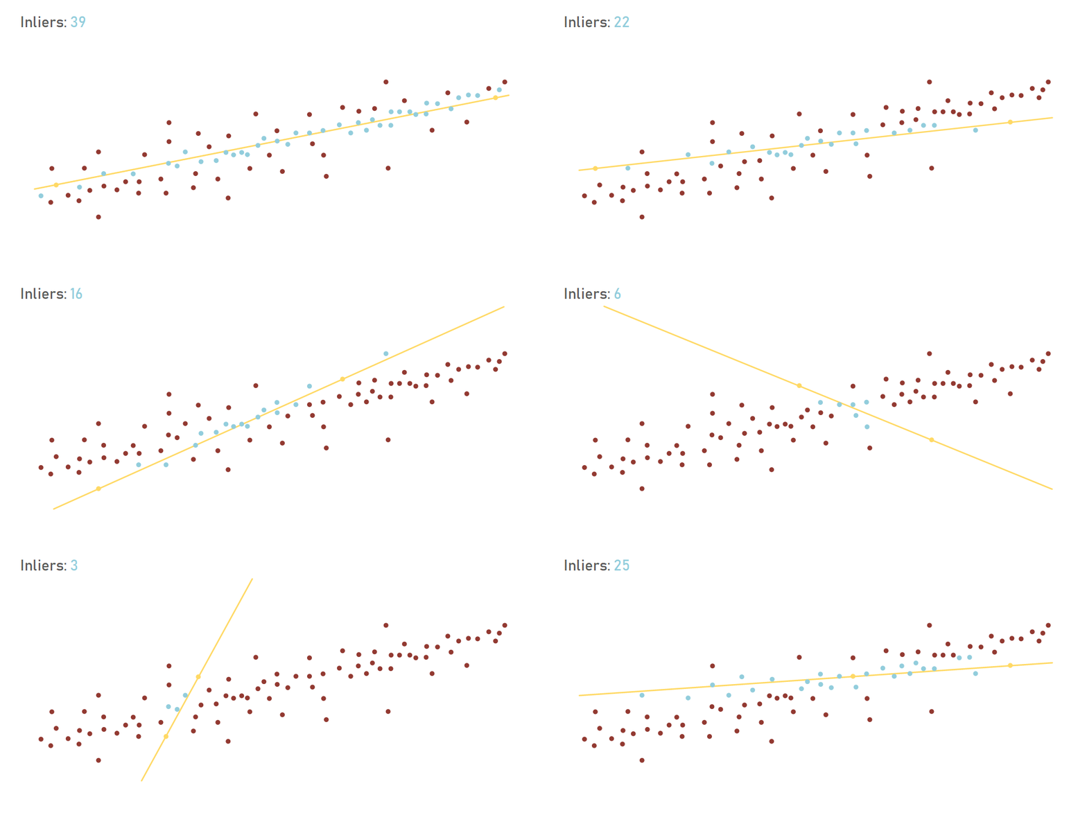
The reason that the RANSAC algorithm was selected for fitting the lines in the segments over linear fitting methods, such as least squares, is robustness. During initial testing it became clear that when the laser rangefinder scans across a dead angle, it would detect points in this area that are not actually on the map. These points should not be taken into account when fitting the line. As visualised above, these outliers are ignored by RANSAC. If a linear fitting algorithm such as least squares were to be used, these outliers would skew the actual line, resulting in inaccurate line detection.
A final line correction needs to be done because the RANSAC function implementation only returns start and endpoints somewhere between the found vertices. The lines need to be fitted so that the corners and endpoints align to the real wall lines. This is simply done by determining the lines between the points and then equate the lines to each other. The final endpoints are determined by equating the point on the line where the found vertices are perpendicular to this line.
The code snippet of the RANSAC function can be found here [6].
World model object
The world model is the central object in the software architecture. The purpose of the world model is to act on changes in the positioning of PICO, such as sensing where on the map PICO is, determining to which pathpoints to drive, and in which direction to drive in order to reach a pathpoint. An additional responsibility of the world model is to visualise the conditioned LRF data and the pathpoint to which PICO is driving, as well as storing snapshots of the LRF data when commanded to do so.
Position estimation
Using the wall finding algorithm as described earlier, it is possible to extract the relative position in cartesian coordinates of all the visible corners. By matching these corners to the known corners from the given json file, it is possible to determine the location of PICO. This is done in one big function containing several steps. This function is constantly running in the background, and determines the absolute position of PICO, with the origin in this frame being determined as the zero point in the json file.
The first step in the localization function is extracting all corner positions from the json file, as well as getting all visible corner positions from the wall finding algorithm function. Of course, these two corner positions will be given in a different frame, and as such, a conversion needs to be made from one frame to another. As such, the coordinates of the corners given from the wall finding algorithm are converted from the relative PICO frame, to the absolute frame, in order to make it similar to the json file coordinates. This may seem as a catch-22 situation, as converting these coordinates from a relative to an absolute frame requires the position and orientation of PICO, which is exactly what the output of this function will be. So the conversion is made using the last correctly found absolute coordinates and orientation of PICO. Since this function is ran with a frequency of 20 Hz, it can be assumed that the last known position and orientation will be close to the new position and orientation.
The rest of the function can be divided into two steps. First, the function will determine the orientation of PICO. Next, the function will determine the position of PICO. For orientation finding, the relative to absolute conversion is made a lot of times using ‘the last known orientation-0.3’ rad to ‘last known orientation+0.3’ rad, with steps of 0.01 rad. This results in a list of sets of corner positions in absolute coordinates found using a lot of different orientations. This list of sets will be compared to corner coordinates from the json file. The next step is to see which set of corners has the least amount of variance in error when compared to the json file. This method is used because the actual absolute position of PICO will be slightly different from the absolute position used in the frame conversion, so there will always be an error. However, it can be assumed that this error should be roughly the same for all corners when the orientation is correct, and as such, the variance should be as low as possible. So all sets of corners are compared to the json file, and the set with the lowest error variance give us the best orientation estimation.
With the correct orientation now known, the correct position can be determined. Two different methods are used in this function, and the average of the results of the two different methods is used as the final solution. The first method used to find the correct position is very similar to the method used for orientation, as this method creates a list of sets of corner position, were the conversion from relative to absolute is made a lot of times using ‘the last known position-1.0’ meter to ‘last known position+1.0’ meter, with steps of 0.1 meter. The steps are followed as with the orientation method, however this time the function will not look at the lowest error variance, but will simply look which set will result in the lowest error.
The second method used to find the correct position goes through all found corners, looks at the found absolute position of these corners, and sees which corner coordinate from the json file is the most similar. This works as the actual absolute position of PICO cannot be too far off from the last known absolute position. When this is done for every found corner, all the errors between the found corners and their best matching json coordinate are compared. It is likely that most of these errors will be roughly the same, with perhaps some errors being totally different. These completely different errors are discarded and only the matching errors are kept. The mean of these errors will be calculated, and the resulting number will be the mismatch between the last known PICO coordinates, and the current real PICO coordinates. The new PICO coordinates can then be saved. The average of the results of this method and the previous method is than taken as the new absolute PICO position.
The function will check if its new position is a realistic result. It does this by comparing it to its previous known position. Since this previous known position cannot be off by too much, it can be assumed that when there is a major difference between the new and old position, something must be wrong. If this is determined, the function will not save the new position, and instead keep the last correct position as its current position. The function will simply rerun with new sensor data to make a new estimation and hopefully, that one will be better. If the function discards the new position several times in a row, it will change some of its control numbers in the function, as to increase the range at which it will search for its correct coordinates. For example, the range of orientation finding will increase from "-0.3 to 0.3" towards "-pi to pi". This wider range numbers are also used when the function is ran for the first time, as during initialization the correct position is only known roughly, and nothing is known about orientation.
The code snippet of the localisation function can be found here: [7].
Path planning
The method of determining the path points is done both automatically and by hand. The program will load the JSON map file when the program starts. The code will detect where all the cabinets are and what the front is of a cabinet. Each cabinet path point will exactly be placed in the middle of the virtual square area that is specified in front of the cabinet. The rest of the path points are put in by hand. A path point has three variables: the x and y coordinates and the direction. The direction only applies when the path point is in front of a cabinet. The orientation that PICO needs to have to be in front of the cabinet is specified within the direction variable. The direction will be subtracted from the real orientation of PICO and is corrected afterwards if PICO is not aligned right. Figure 5.5 shows the modified version of the hospital JSON map.
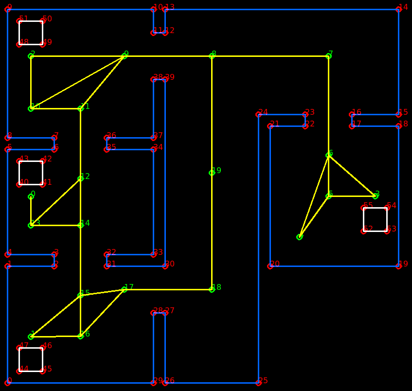
| Point | X | Y |
|---|---|---|
| 0 (cabinet 0) | 0.4 | 3.2 |
| 1 (cabinet 1) | 0.4 | 0.8 |
| 2 (cabinet 2) | 0.4 | 5.6 |
| 3 (cabinet 3) | 6.3 | 3.2 |
| Point | X | Y |
|---|---|---|
| 4 (Start point) | 5.0 | 2.5 |
| 5 | 5.5 | 3.2 |
| 6 | 5.5 | 3.9 |
| 7 | 5.5 | 5.6 |
| 8 | 3.5 | 5.6 |
| 9 | 2.0 | 5.6 |
| 10 | 0.4 | 4.7 |
| 11 | 1.25 | 4.7 |
| 12 | 1.25 | 3.5 |
| 13 | 0.4 | 2.7 |
| 14 | 1.25 | 2.7 |
| 15 | 1.25 | 1.5 |
| 16 | 1.25 | 0.8 |
| 17 | 2.0 | 1.6 |
| 18 | 3.5 | 1.6 |
| 19 | 3.5 | 3.6 |
| Path | Length |
|---|---|
| 4->5 | 0.86 |
| 4->6 | 1.49 |
| 5->3 | 0.8 |
| 5->6 | 0.7 |
| 3->6 | 1.06 |
| 6->7 | 1.7 |
| 7->8 | 2.0 |
| 8->9 | 1.5 |
| 9->2 | 1.6 |
| 9->10 | 1.84 |
| 9->11 | 1.17 |
| 2->10 | 0.9 |
| 10->11 | 0.85 |
| 11->12 | 1.2 |
| Path | Length |
|---|---|
| 12->13 | 1.17 |
| 12->14 | 0.8 |
| 13->0 | 0.5 |
| 13->14 | 0.85 |
| 14->15 | 1.2 |
| 15->1 | 1.1 |
| 15->16 | 0.7 |
| 15->17 | 0.76 |
| 1->16 | 0.85 |
| 16->17 | 1.1 |
| 17->18 | 1.5 |
| 18->19 | 2.0 |
| 19->8 | 2.0 |
In the current design of the point map, there is a possibility that some points cannot be reached because of an obstacle that is on that point. For example, if there is a obstacle on point 8, the path movement from point 7 to point 8 would be impossible to complete. This would mean that the whole left side of the map can not be accessed by the robot, since driving from point 7 to point 8 is required to get there. To solve this problem, a nunber of backup paths were added to the point map. These are paths between points that were not initially connected. These paths are defined such that the robot will only choose it if there are no other options to go to a certain point. The backup paths added are:
| Backup paths |
|---|
| 5->7 |
| 7->9 |
| 8->18 |
Pathpoint route calculation
In the path planning section, the method the robot uses to navigate through the hospital was explained. The robot will use a point map, where each point is connected to a different neighboring point. To get from a point to a non-neighboring point, the robot needs to travel from point to point to get there. This list of points is called the route the robots needs to travel. The pathway between points is referred to as the path. Usually, there are multiple routes from a point to another point. In this case, the shortest route is preferred, since the chance of the robot losing its position on the map is the smallest.
In order to obtain the shortest route, the Dijkstra algorithm is used. This algorithm can be used to obtain the shortest path from a point to another point, given a point map and the weight of the paths between the points. This weight can be based on the distance between the points or the difficulty of the path. Dijkstra's algorithm works by creating a list of the distance from a start point to every other point. The algorithm then checks the distance to each other point, whilst updating the list of shortest distances. The algorithm also remembers the previous point from which the shortest route came. So once the shortest distance list is completed, the algorithm can backtrack the route from the end point to the starting point.
Figure 5.6 illustrates how the algorithm works. Inside the points the current shortest path to the point is indicated, while the number near the path is the weight of that path.
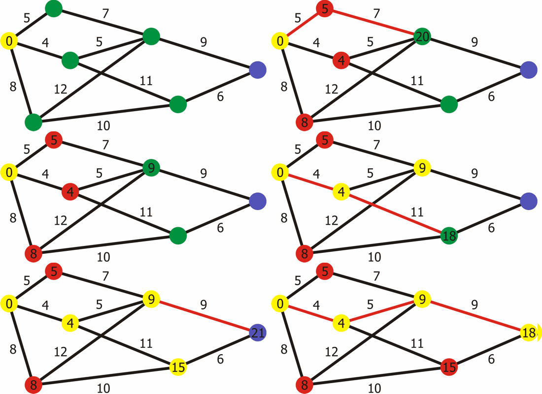
In the software, the point map is represented as a matrix. This matrix contains the distance from each point to every other point. Such an example matrix is shown below. In this matrix, point d[1,n] is the weight from point 1 to point n. Value d[n,1] will be the same, as this is the distance from point n to point 1. If, for example, point 1 and point two would not be connected, the value in the matrix would be d[1,2] = d[2,1] = 0. The weight of the path is represented by a number greater than 0. The greater the number, the more difficult the path. The diagonal of the matrix contains the distances from each point to itself. Therefore, this value should always be zero (d[n,n] = 0).
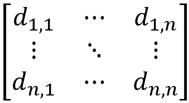
Based on the mentioned properties of the point matrix, it can be concluded that this matrix should always be symmetric and always have only zeroes in the diagonal. These properties can be used when to check whether the inputted map is free of errors. Furthermore, editing the point matrix is simple. If a path between point n and point m needs to be added or removed, all that needs to be done is change the values such that d[m,n] = d[n,m] = w, where w is the new weight of that path. If a path needs to be removed, w should be equal to 0.
Drive target calculation
Now that both the absolute position of PICO and that of the next pathpoint are known on the map, the robot needs to know in which direction to drive. That means that the location of the pathpoint that PICO should drive to, needs to be transformed to the coordinate space of PICO. This way it can be figured out in which relative direction PICO should drive and how much PICO should rotate before driving. The results of the calculations is visualised in figure 5.7.
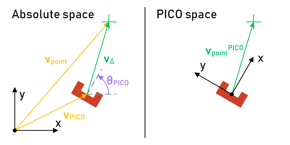
The first step is to determine the difference vector ![]() between the position of the pathpoint
between the position of the pathpoint ![]() and the position of PICO
and the position of PICO ![]() . This is done by a simple subtraction:
. This is done by a simple subtraction:

Then the coordinate space matrix of PICO ![]() needs to be determined in order to create the transition matrix. This is done by using the absolute rotation of PICO
needs to be determined in order to create the transition matrix. This is done by using the absolute rotation of PICO ![]() in order to calculate the unit vector components of the x- and y-axes of the PICO coordinate space within the absolute coordinate space.
in order to calculate the unit vector components of the x- and y-axes of the PICO coordinate space within the absolute coordinate space.

Then the relative position vector of the pathpoint in PICO's coordinate space ![]() can be calculated by multiplying the inverse of the PICO space matrix with the difference vector:
can be calculated by multiplying the inverse of the PICO space matrix with the difference vector:

With the relative coordinates known of the next pathpoint, PICO knows how far to turn in a certain direction before driving and where to aim for when avoiding obstacles. This requires the relative position of the targeted pathpoint to be recalculated every tick, so the driving code can correct for changes in direction in real time.
Visualisation
Several visualisation functions were made for the sake of debugging the trajectory of PICO. These functions are built upon the OpenCV framework and are meant to streamline the process of drawing the LRF data, the detected walls, targeted pathpoints, and PICO itself. These functions require a Mat object as an input (pass by reference) and then they draw their shapes on there. This way, all the data can be passed into these functions using world units without the need for converting everything to pixel positions within the image.
By stacking all the mentioned functions on a single Mat object, the main visualiser of the program was created. A gif of the visualiser in a simulated environment is displayed in figure 5.8. The blue point represents the active target of PICO at any given time. The walls are drawn in white on top of the green LRF data.
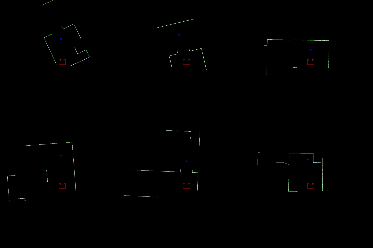
Lastly, a function was made to take snapshots of the LRF data when PICO arrives at a cabinet. These snapshots are written to the "Snapshots" folder in the project directory, and contain information in the filename of the snapshot number and the cabinet number. This function makes use of the function that scatters the LRF data on a Mat object, that was mentioned earlier. The function to draw PICO on the image is also used. The resulting Mat object is then written to a .png file using the OpenCV function "imwrite." An example snapshot that was made in the simulation environment is shown in figure 5.9.
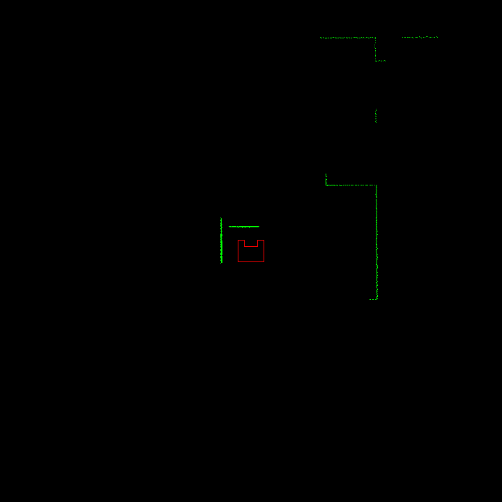
Control object
The control object contains the actuator control, called drive control. This object provides output to the actuators based on inputs from the world model.
Drive control
The actuators are controlled such that the movement of the robot is fluent. This is achieved by implementing an S-curve for any velocity change. The S-curve implementation was chosen to limit jerk in the robot's movement and thus preventing slip. The reduction of slip in the motion of PICO increases the accuracy of its movement on top of the fluency. The S-curve is implemented in two different functions; the function 'Drive' accelerates and decelerates smoothly to a certain speed or rotation in any direction. The second function 'Drive distance' accurately accelerates and decelerates over a fixed distance or rotation. General information on S-curves can be found via the link under useful information.
Drive control has been further incorporated in a function that uses a potential field. This function prevents the robot from bumping into objects in a fluent manner. See figure 5.10 for a visual representation of an example potential field. The leftmost image shows the attraction field to the goal, the middle image shows the repulsion from obstacles and the rightmost image shows the combination of the two. Any wall or object is taken into account for this function.

However, the implementation used for PICO does not use an attraction field, only repulsion from obstacles. The potential field vector is calculated in real-time, as the robot is expected to run into dynamic obstacles in the final challenge. This also takes the imperfections in the physical environment into account. The way the potential field is obtained is visualised in figure 5.11.
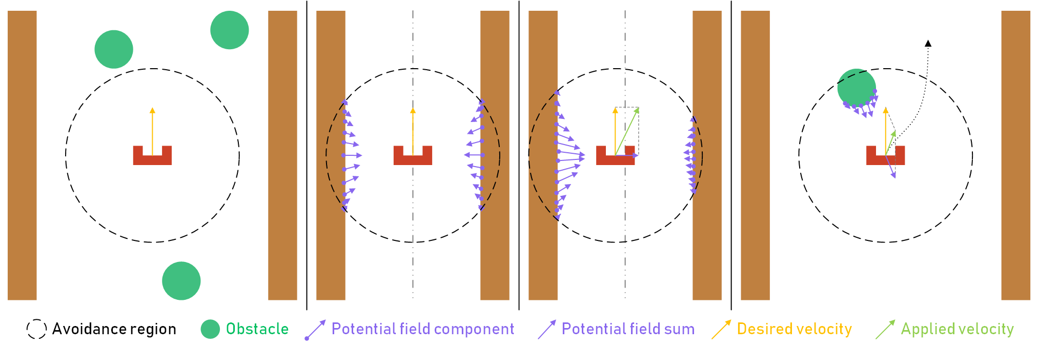
The first image shows how the robot is far away enough from any walls or obstacles, and thus the potential field vector is zero, causing the robot to keep its (straight) trajectory. In the second image, the robot is driving through a narrow corridor. As a result of the symmetry of the environment, the potential field component vectors cancel each other out, causing the potential field sum vector to be zero. Once again, the robot keeps its trajectory. In the third image however, the robot is closer to the left wall, causing the left potential field component vectors to outweigh the right ones. As such, the potential field sum vector points to the right, causing the robot to drive towards the middle of the corridor, until the sum vector reaches its steady state value when the robot is in the middle again. The fourth image depicts a situation where an obstacle, such a random box or a walking person, enters the avoidance region around the robot. Once again, the potential field sum vector points away from the obstacle, causing the robot to drive around the obstacle as depicted by the dotted line.
Although the potential field prevents collision with obstacles, it also pushes PICO off course. To make sure that PICO still reaches its goal, an orientation correction was implemented. This function uses the position data to calculate PICO's orientation relative to its current goal. If this orientation differs from the desired orientation, namely that PICO looks directly at its goal, the difference in angle is corrected.
Testing
This chapter describes the most important tests and test results during this project.
Test Goals
Several tests were executed during the course of the project, each with a different goal. The most important goals are summarised below:
- Test the laser rangefinder and the encoders.
- Determine the static friction in the actuators for the x- and y-direction, and the rotation.
- Collect laser data for the spatial recognition functions.
- Test the drive control functionality, consisting of the S-curve implementation and the potential field.
- Test the full system on the example map.
Results
The results from each test are described in separate parts.
Laser rangefinder & motor encoders
The range of the laser range finder according to the simulation is 10cm to 10m, the angle is +114.6 to -114.6 degrees as measured from the front of the robot. This angle is measured in 1000 parts, per an amount of time that can be determined by the user. However, the actual range is much larger. During the test, laserdata appeared within the 10cm radius of the robot. This data produced false positives and had to be filtered out. The maximum range of the range finder was actually larger than 10 meters, but this does not limit the functionality of the robot. The other properties of the laser range finder were accurate.
The values supplied by the encoders are automatically converted to distance in the x- and y-direction in meters and a rotation a in radians. Due to the three wheel base orientation of the actuators, the x- and y-direction movement estimation are less accurate than that of the the rotation.
Static friction
The actuators have a significant amount of static friction. The exact amount of friction in both translational and the rotational direction was difficult to determine. An attempt was made by slightly increasing the input velocity for a certain direction until the robot began to move. This differed for each test, so the average was taken as a final value for the drive control code. It is important to note that the friction was significantly less for the rotational direction than the translational directions. The y-direction had the most friction and also had the urge to rotate instead of moving in a straight line, especially at low velocities.
Laser data
Due to the limited testing moments, some laserdata was recorded in different situations. This data could be used to test the spatial recognition functions outside the testing moments. Data was recorded in different orientations and also during movement of the robot.
Drive control
This test was executed to determine if the smoothness and accuracy of the drive control functions were sufficient or if the acceleration would have to be reduced. Both the smoothness and the accuracy were satisfactory, especially for the rotational movement.
The potential field was also tested by walking towards the robot when it was driving forward. It successfully evaded the person in all directions while continuously driving forward.
Full system test
The full system test was executed on the provided example map. However, during this test, no dynamic or static obstacles were present that were not on the map. PICO was able to find the cabinets in the correct order from different starting positions and orientations, but the limited space between the two cabinets provided some difficulties. Since PICO is supposed to return to its previous navigation point if the orientation in front of a cabinet failed, and this point was in between the two cabinets, this caused some issues. However, in the Hospital challenge map, no two navigation points were placed as close together as in the example map, which should circumvent this issue.
Conclusion & Recommendations
In conclusion, the software implementation of the design described in this Wiki is capable of fulfilling the basic functionality of the hospital challenge. That is, if the hospital environment only contains the necessary wall geometry and the cabinets. The addition of static and dynamic obstacles proved difficult to handle by the position estimation code, and ultimately led to the robot miscalculating the orientation at the end of the hospital challenge.
It is recommended to dedicate the last week before the challenge to testing all the integrated code. This is because the software described in this Wiki was only ever fully implemented during the challenge itself, and the execution proved that the robot was still susceptible to disturbances in the environment in the form of dynamic obstacles. This could have been prevented by fine-tuning several variables in the code. Secondly, it is recommended to dedicate the most time and resources to the position estimation, as this is a crucial element that is relied upon for decision-making in the state machine and calculating the movement trajectory. The potential field implementation, however, proved very robust and simple to implement. It is therefore recommended to other groups to implement this to avoid collision with static and dynamic obstacles.
As a group, we take pride in the fact that we were the only group that managed to land in the top 3 of best performing challenge executions at the end of both the escape room challenge and the hospital challenge.
Appendices
This chapter contains some documents that are of minor importance to the project.
Useful information
PDF of initial Design Document
Minutes
This document contains the minutes of all meetings: Minutes