Embedded Motion Control 2013 Group 11: Difference between revisions
| (138 intermediate revisions by 5 users not shown) | |||
| Line 24: | Line 24: | ||
<td>Talha Ali Arslan</td> | <td>Talha Ali Arslan</td> | ||
<td>0867550</td> | <td>0867550</td> | ||
<td>[mailto: | <td>[mailto:t.a.arslan@student.tue.nl t.a.arslan@student.tue.nl]</td> | ||
</tr> | </tr> | ||
<tr> | <tr> | ||
| Line 33: | Line 33: | ||
</table> | </table> | ||
= Maze challenge evaluation = | |||
The program used to successfully find the exit of a maze was insufficient. The robot entered the first crossing where it encountered a small pocket left and right of the path. Since the pockets left and right where very small, it should go straight since the program neglects pockets which are not useful to explore. Thus the robot continued and wanted to exit the first crossing but it stopped moving when it wanted to exit the crossing. Normally this should not happen. For driving out of the crossing there are three different states where it can be in. Somehow, at first it entered the first state where it follows the right minimum to position itself into the path, after that it changed state (which should not be possible) and this resulted in the fact that it lost its current state and the robot just stopped. Of course in the second trial the same problem should occur, and it did. The day before the maze challenge we added another if() statement which caused this problem and we knew it before the second trial, but we thought that we could not change the code between the two trials. | |||
When the challenge was finished, we did a third trial, of the records, were we erased that extra if() statement. After that, the robot was able to continue, detected both the arrows but at the end it did not go to the exit unfortunately.... | |||
== | = Discussion and Possible Solutions = | ||
= | [[File:video.jpg|left|link=http://www.youtube.com/watch?v=MNNZ6KVImGg]] | ||
'''* http://www.youtube.com/watch?v=MNNZ6KVImGg''' | |||
| Line 72: | Line 61: | ||
== Program Structure == | |||
Already before the corridor challenge we divided the program into nodes. We did this because the code we wrote for the corridor challenge became very large and it was hard to keep the overview of the code. Furthermore we realized that if we divide the code into parts we can split responsibilities easier. In the end the total program was divided into the nodes as shown below. | |||
The division of the program into these nodes helped us a lot because everyone had the overview of the function of each block and it was easier to debug the entire code. We documented the message types of the topics between the nodes and we described the function of each node. | |||
The whole ´pipeline´ is updated on a rate of 40Hz, every time a new laserdata frame is received all the callback functions are called and the processed data or decisions are published. It is of no use to update the pipeline with a higher rate than 40Hz because the data is not refreshed with a higher rate. With the pipeline all nodes are meant except for the camera node. The camera node works with a refresh rate of 30Hz, the update rate of the camera on the jazz robot. | |||
Because the refresh rate of the pipeline is 40Hz the calculation time of each node is limited. Each node has a maximum of 1/40th of a second to publish the processed data and read the new data from the buffer. If the nodes would use more time the buffers in ROS would overflow and data will be lost resulting in inaccuracy and errors. Because the CPU used is so powerful the most expensive calculation in the pipeline is (only) processing a 1080 byte vector the limited time is not a problem. Furthermore, the splitting of the program in nodes assures the time limit will not be reached. | |||
The only time crucial node would be the Camera node. But because the camera refreshes on another rate and so the Camera node is not a link in the pipeline this is no problem either. | |||
In the beginning there was some doubt whether the structure would not introduce too much delay. The delay introduced by the whole pipeline proved to be negligible. All nodes introduce a delay of one frame, except for the Averaging node, this one introduces 3 frames of delay because it takes the average of three laserdata frames. The total delay is 8 frames which corresponds to .2 seconds and an approximate distance of 4cm at a velocity of .2m/s. | |||
All nodes have a specific function which is described below. As is depicted in the program structure there is a node called Mapper. The mapper is implemented as a function in the node Decision Making but can be seen as a node. Implementing the Mapper as a function proved to be more convenient and gave us more freedom considering the data generated in this node is needed in the algorithm of Decision Making. | |||
[[File:ProgramStructure.png|thumb|center|300px|]] | |||
The nodes and topics are described in the following document: | |||
[[File:EMC_Main.pdf]] | |||
== Smoothing Node == | |||
Here, the raw laser data is smoothened using a moving average. This is done by averaging each value from the laserscanner with its neighbours, which leads to data with less noise in it, which is sent to the Averaging node. | |||
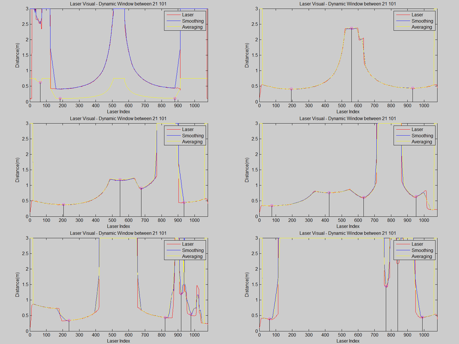
[[File:laser_phenomena.gif|right|]][[File:mov_size21.gif|left|]] [[File:mov_size101.gif|center|]] | |||
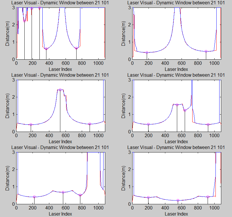
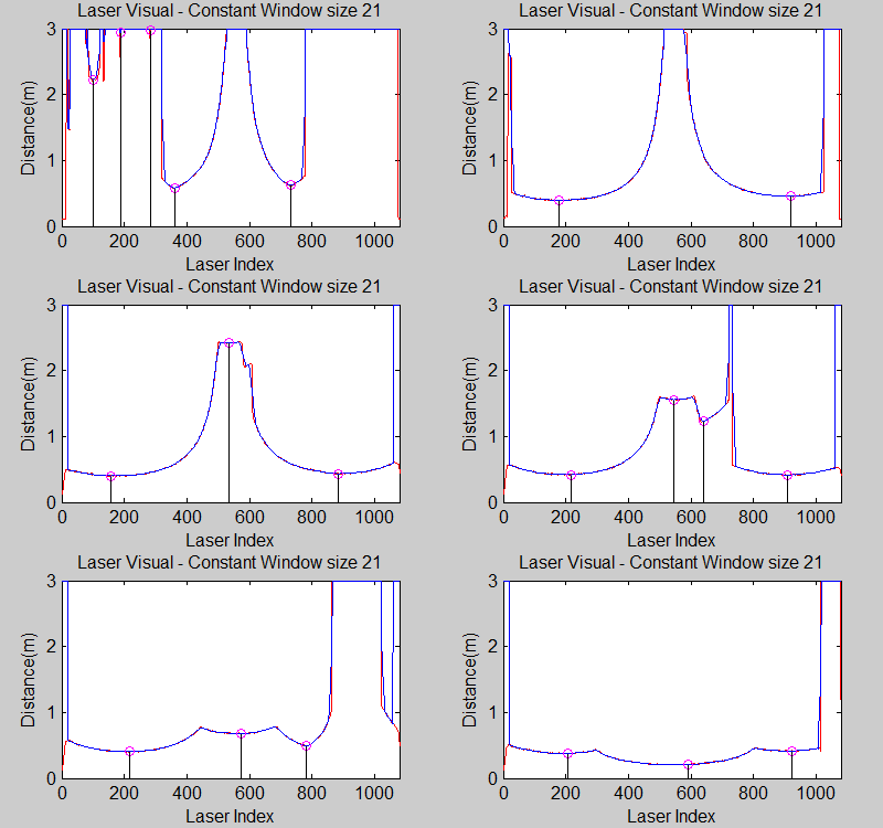
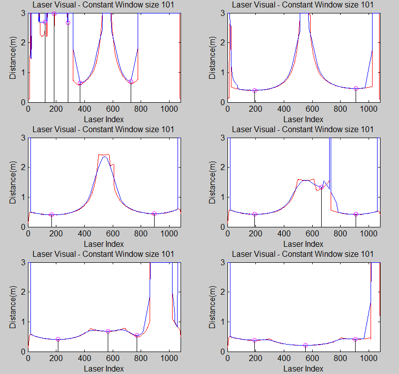
The smoothing is done by applying the moving average method in a variable window size. In this method, moving average at every index is calculated by taking the sum of 'window size' number of elements to the left and right (combined) of that point and dividing it by the window size (i.e. if the window size is 21, 10 points to the back, 10 points to the front and the current point is taken into account). We first started with a constant window size, but there were problems. Because the resolution of laser readings is high over small portions at close distances and low over large portions at large distances, we had to adjust the moving average window size accordingly. In these gifs on the upper left and center, you will see what happens if we use a small and large window size at close distances (Look at with small window size how the minima index changes rapidly and how smoothened the data is, and at large window size, look at how the data is smoothened and there not that much rapid change in minima location as with smaller window size, but there is still movement and this will be overcome in the next node 'Averaging Node'). | |||
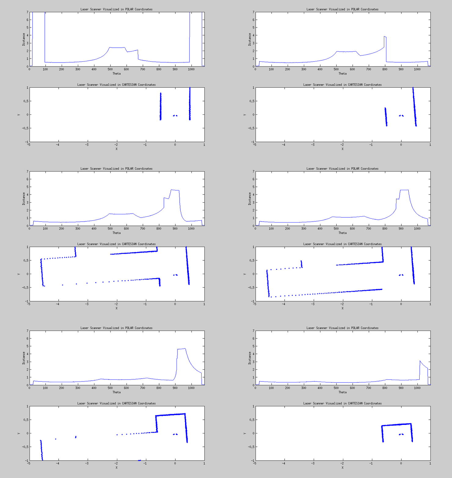
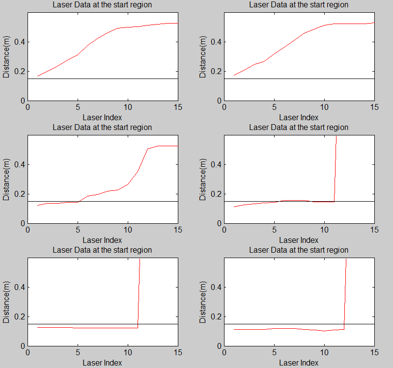
One of the first assumptions was that the laser data below a magnitude of 0.15 m is due to the body of the robot. This is only correct for large distances. In the simulation this holds everywhere but in the real world, we discovered that at close distances first indices of the laser read distances 'between' the actual distance and 0; they look like an interpolation between 0 and those distances and we do not know why this happens; we guess that it may be due to the white shiny surface of the robot case that beams can reflect and be effective at close distances or it may just be a bug of the laser. So; because we depend our smoothing of laser data and determination of local minimum and maximum distances based on these start and finish indices, we should no longer use a dynamic start index and based on real world testing, we should constantly avoid first and last (~approximately) 20 indices which are around 18 in the simulation. We can increase these values based on readings (if a reading below 0.15m still comes after 20th index, we may shift starting index to that value but it should never be below 20). This gif file on the upper right shows the phenomena; where at first the distance to the wall is close, and when the distance increases the problematic readings goes below the line of 0.15 m (black) which was our previous assumption. | |||
The gif pictures below show the whole data and the effect of window size on smoothing. Basically it is seen that with small window size, the smoothened data resembles the original more (not oversmoothened) but at close distances location changes too rapidly and even multiple maximas are found close to each other in some instances. Using a larger window size gives advantage at close distances and flat surfaces, but you can see in the middle gif that data is over smoothened and some corners to the sides are dislocated too much. Below right show a dynamical window result, at distances above a certain distance constand window size is used but between a preferred distance region, window size is proportionally changed between 21 and 101 in this case. Using a very large window size is also not preferable because it increases computation time. Because we use dynamical window, we cannot use a moving array which would solve that problem actually. | |||
How the local minimum values are found is explained in the 'DeterminePosition Node' part. | |||
[[File:all_dyn_21_101_test2.gif|right|]][[File:all_const_21_test2.gif|left|]][[File:all_const_101_test2.gif|center|]] | |||
== Averaging Node == | |||
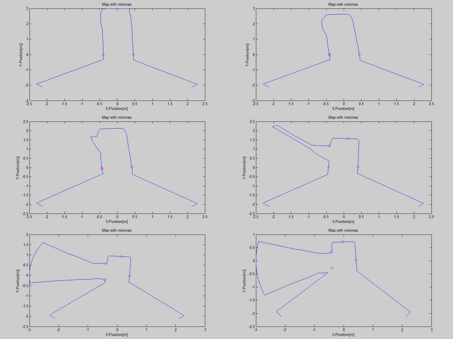
[[File:all_dyn_21_101_test3_with_smooth2.gif|upright=0.3||center|]] [[File:all_dyn_21_101_test3_with_average.gif|upright=0.3||center|]] [[File:Test1.gif|upright=0.3||center|]] | |||
In contrary to the Smoothing node, which averages over all the laser data from a single time instance, this node averages the already smoothened data over several time steps. This is necessary because if there is a disturbance in a single timestep (a large dust particle in front of the laser for instance), we don't want the program to detect things that aren't there. The Averaging reduces the effect of such disturbances. The smoothened, averaged data is then sent to the Determine Position node. | |||
In the visuals above, one can see that averaging helps reduce the oscillation of the minimas. | |||
== Determine Position Node == | |||
Here, the smoothened and averaged data is analysed. The minima and maxima of the laser data are determined, as well as their corresponding indices. This data is sent to the Detect Crossing node. | |||
In this node, every data point from the Averaging node is checked according to its distance and index, relative to the other points within a constant window, where the current point is in the center. Also local maximas or minimas next to each other who have same distances are avoided and only one is taken into account, because from the smoothened and averaged data, there can be points next to or close to each other with same distance value. | |||
Result of this node can be seen in the gif pictures in 'Smoothing Node' and 'Averaging Node' where local minimas are plotted with a circle and a vertical line. | |||
== Detect Crossing Node == | |||
As is presented in the program structure above there is a node which detects the crossings/intersections in the maze. This node detects at which moment PICO is at the middle of a intersection and if there is a side-path on its left and/or right and/or a path in front. | |||
=== Detection of an intersection === | |||
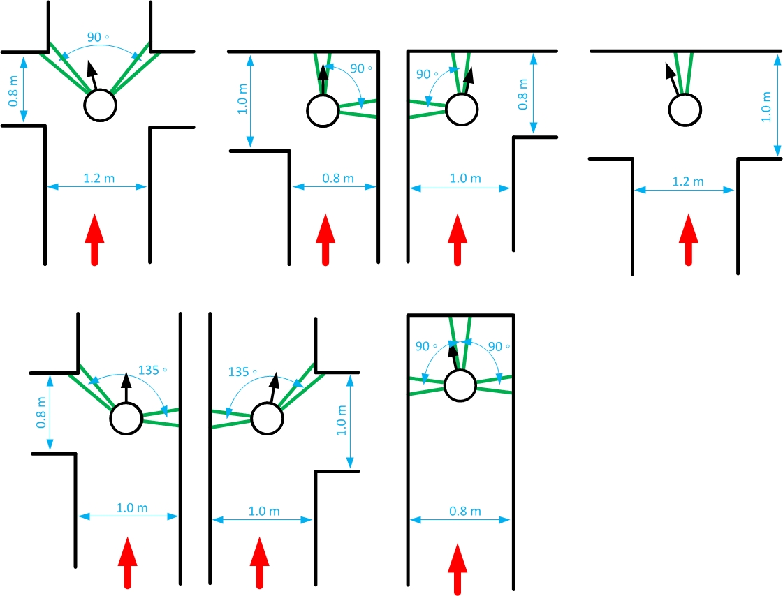
The different types of intersections are detected using a search algorithm. It will look for certain combinations of minima at certain angles. The positions of these local minima are found in the 'Determine Position' node and send via a topic to this 'Detect Crossing' node. The local minima which are found by the 'Determine Position' node will be filtered using a certain treshold. Only the minima which are relatively close to the robot are of interest for detection of the intersections. This treshold depends on the pathwidth which is determined using the laserdata. | |||
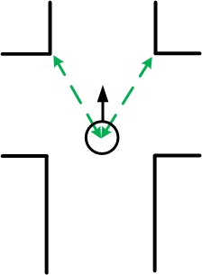
For example, the four-way-intersection which is the first intersection displayed in the figure below is detected using the two minima of the corners in front. The angle between these minima should be approximately 90 degrees and both minima should be at an angle of approximately 45 degrees with the centerline of the path in which the robot is driving. If the robots pointing direction is not parallel with the centerline of the path the angles at which the detection node searches for the minima is adapted accordingly. Since the minima cannot be detected perfectly and since the angular position of the robot cannot be estimated perfectly a detection region is used for detecting these minima. This detection region is illustrated by the green lines in the figures and the width of this detection region is two times delta. With delta being a tuned parameter which was set on 15 laserscanner data increments. | |||
Since there are multiple types of intersections, the node searches for different combination of minima at certain angles at the same time when it is driving through a corridor. The types of intersection which can be detected and the according combination of minima are displayed in the figure below. | |||
[[File:DetectCrossing_start_turn_distances.jpg|center|750x750px]] | |||
Above is explained how the different types of intersections are detected when PICO is driving through a corridor. The Detection node communicates to the DecisionMaking node, which is decribed later on, that it is at the approximate middle of an intersection and which options there are to take; go left, go right, go straight and/or turn around. | |||
=== Detect when a turn is made === | |||
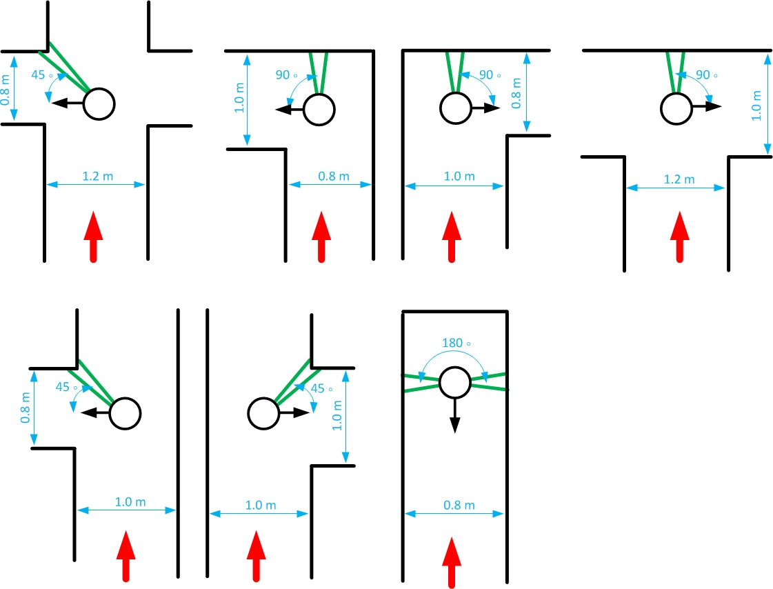
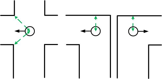
When the Decision Making node decides to go straight on it is not necessary to make a turn and the Drive Safe node, which will be elaborated further on, will be activated directly and PICO continues its way in the same direction. If the Decision Making node decides to make a turn, the Make Turn node is activated and PICO starts to turn. The Detect Crossing node looks if there is a single minimum at a certain detection region while PICO is turning (see images in the figure below). Note that for the dead-end "intersection" the algorithm will look for two opposite minima instead of only one minima at a certain angle. The detection algorithm will search for this single minimum at any time however this information will only be used in the Decision Making node when the robot is making a turn. Let's continue with the example described above, PICO is at the approximate middle of a four-way-crossing and the DecisionMaking node decides to make a left turn. Then the robot will start to turn left untill another minimum is at an angle of 45 degrees in clockwise direction w.r.t. the robots pointing direction. This situation is illustrated in the most upper left image of the figure below. The other images illustrate the detection of a (different) single minimum which indicate that the particular turn is made. Note that the detection of when to stop turning is always done using one minimum which is also used to detect the intersection itself. In this way varying pathwidths will not cause any problems during turning, which is described more elaborately in the last section of this chapter. | |||
[[File:DetectCrossing_end_turn_distances.jpg|center|750x750px]] | |||
=== Early dead-end detection === | |||
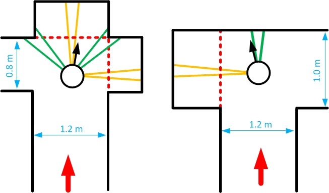
When the detection algorithm detects a certain type of intersection it will also look for possible (short) dead-end corridors. Suppose the robot is at the approximate middle of the intersection displayed in the left image of the figure below. Without the early dead-end detection the Detect Crossing node would detect the intersection as a four-way-crossing using the two minima within the green detection regions. However, an early dead-end detection algorithm is included in the detection node. When PICO is at an approximate center of an intersection, the early dead-end detection checks if there are minima within a certain distance in possible side/front paths. These regions of detection are illustrated by the orange lines. If a minimum within a close distance is detected in a possible side or front corridor, PICO will not see this short dead-end as a possible way to go. Thus the detection algorithm will see the intersection depicted in the left image in the figure below as an intersection with only a path to the left (this is illustrated using the dashed red lines). Thus the only option which the Decision Making node will have is to turn left. The right image in the picture below shows another example of early dead-end detection. | |||
[[File:DetectCrossing_earlydeadend_distances2.jpg|center|500x500px]] | |||
=== Robustness for variable pathwidth within a maze === | |||
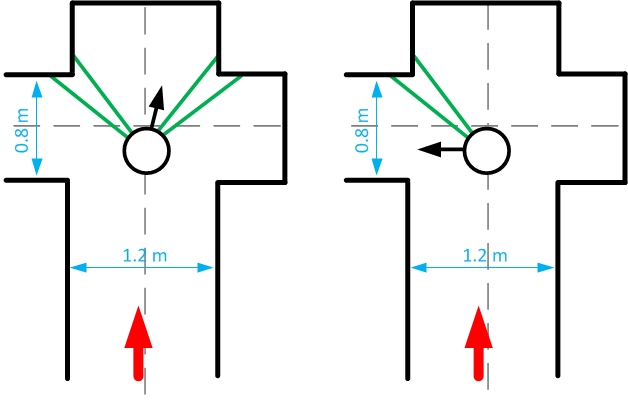
Since the pathwidth within the maze was not known beforehand it was necessary to implement some adaptation into the program. We tried to design our program in a way such that it can handle various pathwidths. It was communicated to us that the pathwidth within the maze could vary with +/- 15 centimeter, therefore we also thought about how to cope with these pathwidth differences. In the figures shown above is shown that the detection still works even if the pathwidths of the corridors within the maze differ for 20 centimeter or even more. This is also shown using the figure below. The dashed grey lines indicate the centerline of a corridor . If the robot is driving through a corridor it will approximately follow the centerline of this particular corridor . When the intersection is detected and a turn is made, using the method described earlier on in this chapter, the robot is not at the centerline of the corridor which it will enter. However this is no problem since the Drive Safe node will correct for this while driving into this corridor, which is described in the chapter about the Drive Safe node. | |||
[[File:DetectCrossing_robust_distances.jpg|center|500x500px]] | |||
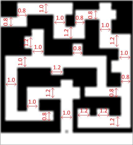
To see the crossing detection in action see the link below. The different pathwidths are illustrated in the figure below. | |||
* http://www.youtube.com/watch?v=wn6UfZ8Y5io | |||
[[File:VariablePathwidth.jpg|center]] | |||
== Decision Making Node (UNDER CONSTRUCTION) == | |||
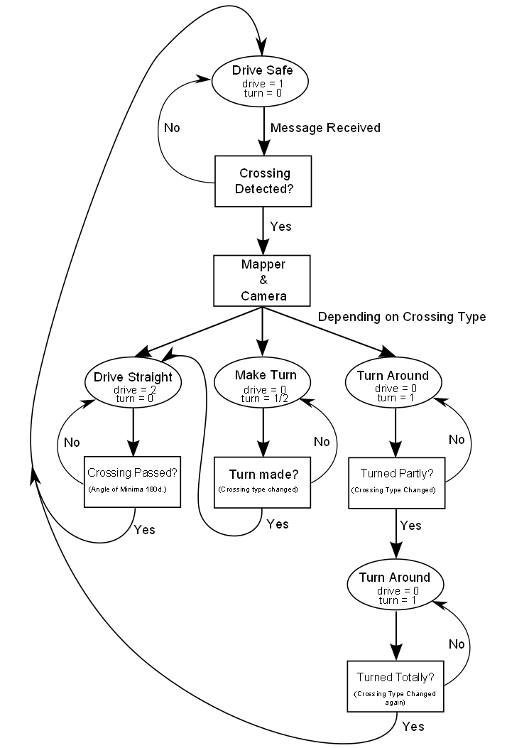
The Decision Making node is the connecting node of the whole structure, in other programs called the 'brains' or 'master' node. This node contains the strategy to solve the maze and uses the Camera arrow detection and info stored in the Mapper to find the fastest way out of the maze. As depicted the program is state-based. There are four main states; Drive Safe, Drive Straight, Make Turn and Turn Around. | |||
When the Decision Making is in the states Drive Safe or Drive Straight the Drive Safe node is activated. In the state Drive Safe the robot is driving in between two walls. The Decision Making sends a '1' to the Drive Safe node and a '0' to the Make Turn node. The Decision Making leaves this state when a crossing (including dead-end) is detected. In this state the Drive Safe node orientates on the minima on the sides of the robot. | |||
In the state Drive Straight the Decision Making node sends a '2' to the Drive Safe node and a '0' to the Make Turn node. By sending a '2' to the Drive Safe node the node orientates using the correct minima for each crossing. | |||
In both Drive-states the robot has mostly linear velocity and all angular velocity is controlled by the Drive Safe node. When the Drive Safe node receives a '0' it will stop publishing on the base control topic. | |||
When the Decision Making is in the states Making Turn or Turning Around the node sends a '1' or '2' to the Making Turn and a '0' to Drive Safe. The value sent determines the direction the robot will turn. This means that the robot has only angular velocity and turns on it's base. The Decision Making node leaves the Making Turn state when Detect Crossing detects the correct crossing. | |||
The state Turning Around is developed especially for when the robot encounters a dead-end. The robot needs to turn 180 degrees and during turning two particular situations must occur subsequently before the robot is turned completely. The crossing type published by the Detect Crossing should change twice, first to 'Right' and then to 'Straight'. | |||
[[File:NodeStructure.png|thumb|center|500px|]] | [[File:NodeStructure.png|thumb|center|500px|]] | ||
===Mapper=== | |||
To see the mapper node in action: | |||
* http://www.youtube.com/watch?v=h5qNmMapMB4 | |||
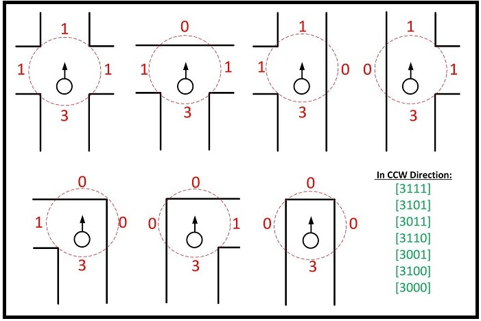
It is easy to remember which turns robot has made over time and to manipulate its choices by always making a specific turn or balancing them. However the task of remembering where it has come from and what choices remain is rather complex. For this we tried to simplify the problem as much as possible. At every new node, a term is added to the map which is kept as an [some constant][node count] size array. When the robot crosses a node, map is updated on that node, so that when the robot comes back, it knows which direction it has come from, where it can go and cannot go. When a dead end is reached, it reflects back on previous nodes too and as robot makes its way back to the last node where there is an option to go to, nodes are erased from the array. So, in the end, if the robot makes it out of the maze, we have an array with smallest amounts of nodes in it, and with 'dead end' information in them. | |||
Every node is defined as 4 term vector: | |||
[current , right of the current , ahead of the current , left of the current] | |||
[[File:Mapper2.jpg|Left|]][[File:Mapper.jpg|Right|]] | |||
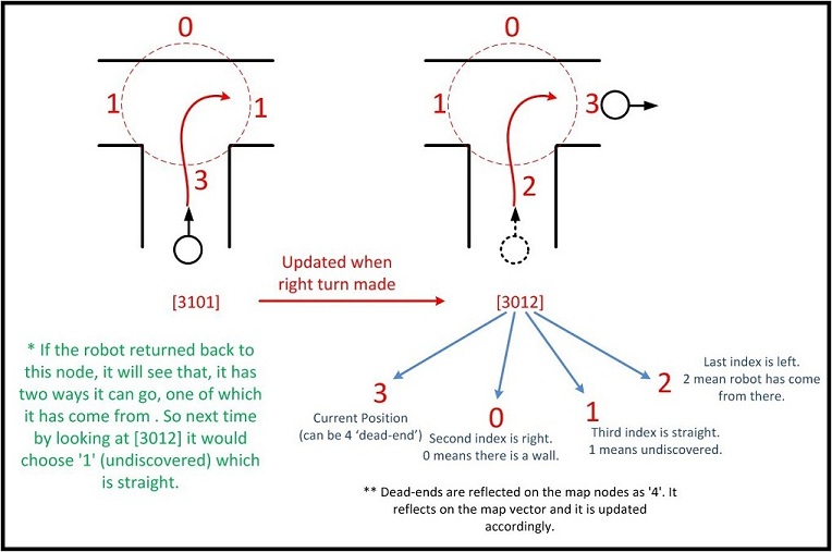
It is simply a record of ways in counterclockwise directions. The term current 'Current' is where the robot is and it can either be 3 or 4 (4 means that there is a dead end behind the robot and it is returning). Other terms can be 0,1,2,4. 0 means there is no opening (wall). 1 means it is an option that is not discovered yet. 2 means robot has come from there before. 4 means there is an opening but it has dead end(s). | |||
As an example 'T crossing' is defined as [3101]. Current direction is 3, the one to the right is 1 (there is an opening), ahead is 0 (wall), left is 1 (there is an opening too). As another example, a right corner is defined as [3100] or a left corner [3001] or when the robot drives between walls [3010] (but this is not added to the map other than the start). If there is a 4-way crossing it is [3111]. | |||
If the robot crossed a new right corner, it first detects it as [3100] and when it makes the turn and passes it, map updates that term to be [3002]; because now it has become a left turn. Same with if the robot makes a left turn at a 4-way crossing [3111] after the node is passed, that node will be updated as (it turned left so now it is as if it has come from the right), [3211]. Take for instance the node type of [3110] where the robot can continue straight or right and there is no opening on its left. If it makes the right turn, (if it comes back to that node) the wall will be at its front, the option that it did not go before will be on its right and its previous choice will be on its left; [3102]. When the robot gets to dead ends, it updates current 3 as 4 and this effects previous nodes too. As an example at an 4 way crossing in the maze at the very start, we assume for the maze competition that on of them can be the correct one. Initially it will be [3111] and if we are not so lucky, we are going to eliminate all the dead ends and the node will become for example [4241]. 2 is where the start of the maze is (on the right) and this means that if we chose the option straight ahead at first it could have saved us time. | |||
So discovering the maze requires a strategy of choosing between the undiscovered options, but returning from dead ends requires only remembering the nodes and making our way back to a desired node correctly. | |||
== Drive Safe Node == | |||
The Drive Safe node makes sure that PICO drives safely throughout the whole maze. This means that PICO drives safely between walls so that it does not hit a wall and drives optimally through the pathway, it detects when it is entering a crossing and drives safely and straight to the middle of the crossing, and after PICO made the correct turn it exits the crossing safely and straight. After it exits the crossing, it continues to drive safely between walls. | The Drive Safe node makes sure that PICO drives safely throughout the whole maze. This means that PICO drives safely between walls so that it does not hit a wall and drives optimally through the pathway, it detects when it is entering a crossing and drives safely and straight to the middle of the crossing, and after PICO made the correct turn it exits the crossing safely and straight. After it exits the crossing, it continues to drive safely between walls. | ||
| Line 137: | Line 191: | ||
Note that all thresholds are tuned during the real-time experiments | Note that all thresholds are tuned during the real-time experiments | ||
=== Normal Driving === | |||
PICO is in the `Normal Driving' mode if PICO is located between walls. In order for PICO to take the turns correctly, PICO should remain approximately in the middle of the path with its forward position parallel to the walls before it will be in the `Enter Crossing' mode. To determine when PICO is located between walls, we know that there are at least two minima which are approximately 180 degrees apart (approximately since the noise disturbs the Determine Position node). If those two minima are indeed approximately 180 degrees apart PICO is between walls, and if this is not the case (the angle between the two minima differs to much with a certain threshold) PICO enters a crossing. Also if one of the minima becomes to small, PICO goes into the Safety Driving node. | PICO is in the `Normal Driving' mode if PICO is located between walls. In order for PICO to take the turns correctly, PICO should remain approximately in the middle of the path with its forward position parallel to the walls before it will be in the `Enter Crossing' mode. To determine when PICO is located between walls, we know that there are at least two minima which are approximately 180 degrees apart (approximately since the noise disturbs the Determine Position node). If those two minima are indeed approximately 180 degrees apart PICO is between walls, and if this is not the case (the angle between the two minima differs to much with a certain threshold) PICO enters a crossing. Also if one of the minima becomes to small, PICO goes into the Safety Driving node. | ||
The two minima (index and distance, indicated by the red lines) are used to determine the width of the path (orange line), the position from the middle of the path (difference between the green and blue line, left from the blue line is negative) and the angle between the forward position and the right wall and the left wall (purple lines). Those are depicted in the figure below. | The two minima (index and distance, indicated by the red lines) are used to determine the width of the path (orange line), the position from the middle of the path (difference between the green and blue line, left from the blue line is negative) and the angle between the forward position and the right wall and the left wall (purple lines). Those are depicted in the figure below. | ||
[[File:DriveSafe.jpg|left]][[File:straight.jpg|right]][[File:exponent.jpg|center]] | [[File:DriveSafe.jpg|left|300x300px]][[File:straight.jpg|right|300x300px]][[File:exponent.jpg|center|300x300px]] | ||
| Line 177: | Line 231: | ||
Of course <math>\beta</math> can be chosen very high so that PICO returns quickly to the middle of the path, however from real-time experiments was observed that PICO has an overshoot due to a certain delay. Therefore <math>\beta</math> and the constant are tuned so that PICO moves to the middle of the path without oscillating around the middle. | Of course <math>\beta</math> can be chosen very high so that PICO returns quickly to the middle of the path, however from real-time experiments was observed that PICO has an overshoot due to a certain delay. Therefore <math>\beta</math> and the constant are tuned so that PICO moves to the middle of the path without oscillating around the middle. | ||
=== Entering Crossing === | |||
When the two minima do not make an angle of approximately 180 degrees and PICO was in the Normal Driving state before, PICO enters a crossing. From the location of the different minima that are observed can be determined what type of crossing it enters. | When the two minima do not make an angle of approximately 180 degrees and PICO was in the Normal Driving state before, PICO enters a crossing. From the location of the different minima that are observed can be determined what type of crossing it enters. | ||
==== T-crossing, left turn or right turn ==== | |||
If there is one minimum detected approximately at index 540 (within the threshold of course), we know that there is a wall in front of PICO. The only thing we want is that PICO drives towards this minimum so that drives straight into the crossing and can detect a crossing accurately using the DetectCrossing node. So the angular velocity is adapted so that the minimum will be detected around index 540 the whole time. The figures below show the different crossing when it should go to the minimum at index 540. So we correct the angle of PICO, for instance if the minima is at index 580, we know that PICO is oriented to the left, and we give it an angular velocity to the right. | If there is one minimum detected approximately at index 540 (within the threshold of course), we know that there is a wall in front of PICO. The only thing we want is that PICO drives towards this minimum so that drives straight into the crossing and can detect a crossing accurately using the DetectCrossing node. So the angular velocity is adapted so that the minimum will be detected around index 540 the whole time. The figures below show the different crossing when it should go to the minimum at index 540. So we correct the angle of PICO, for instance if the minima is at index 580, we know that PICO is oriented to the left, and we give it an angular velocity to the right. | ||
[[File:frontminimum.jpg|center]] | [[File:frontminimum.jpg|center]] | ||
==== Left turn or right turn with a straight path ==== | |||
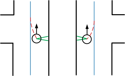
If there is no minimum approximately at index 540, and if there is one minimum detected approximately at index 180 (right), or one minimum detected approximately at index 900 (left) and not both at the same time of course otherwise we are between walls, then we know that PICO enters a crossing where you can turn right or straight and respectively left or straight. Since the width of the path can not be measured in the crossing, the old width of the path is remembered and the same strategy is used as in the Normal Driving state to drive to the middle of the path and to drive straight with respect to the wall (right or left). | If there is no minimum approximately at index 540, and if there is one minimum detected approximately at index 180 (right), or one minimum detected approximately at index 900 (left) and not both at the same time of course otherwise we are between walls, then we know that PICO enters a crossing where you can turn right or straight and respectively left or straight. Since the width of the path can not be measured in the crossing, the old width of the path is remembered and the same strategy is used as in the Normal Driving state to drive to the middle of the path and to drive straight with respect to the wall (right or left). | ||
[[File:leftright.jpg|center]] | [[File:leftright.jpg|center]] | ||
==== Three-way crossing ==== | |||
If the T-crossing, left turn, right turn, left turn or right turn with a straight path do not occur, then PICO enters a three-way crossing. Now we need to use the two minima which are in front of PICO but the number of minima can vary between 2, 3 or 4 minima in the threshold. Also the index of two minima in front of PICO will change when PICO enters the crossing. Therefore, depending on the number of minima in the threshold, the right minima are selected and the angular velocity is changed such that the distances to these minima become equal. So if the left minima of the two is further away than the right minima, then PICO should be oriented to the left and should drive forward. | If the T-crossing, left turn, right turn, left turn or right turn with a straight path do not occur, then PICO enters a three-way crossing. Now we need to use the two minima which are in front of PICO but the number of minima can vary between 2, 3 or 4 minima in the threshold. Also the index of two minima in front of PICO will change when PICO enters the crossing. Therefore, depending on the number of minima in the threshold, the right minima are selected and the angular velocity is changed such that the distances to these minima become equal. So if the left minima of the two is further away than the right minima, then PICO should be oriented to the left and should drive forward. | ||
[[File:threeway.jpg|center]] | [[File:threeway.jpg|center]] | ||
=== Exiting Crossing === | |||
When PICO is entering a crossing, a Drive message of 1 is published by the Decision Making node. At a certain point, the Detect Crossing node detects a crossing and the Decision Making node publishes a Drive message of 0 and PICO is will make a turn accordingly. During the Drive message of 0, PICO does not drive, and only turns. When the turn is finished, a new Drive message of 2 is published by the Decision Node and PICO is in the Exit Crossing state. | When PICO is entering a crossing, a Drive message of 1 is published by the Decision Making node. At a certain point, the Detect Crossing node detects a crossing and the Decision Making node publishes a Drive message of 0 and PICO is will make a turn accordingly. During the Drive message of 0, PICO does not drive, and only turns. When the turn is finished, a new Drive message of 2 is published by the Decision Node and PICO is in the Exit Crossing state. | ||
| Line 208: | Line 262: | ||
[[File:exitcrossing.jpg|center]] | [[File:exitcrossing.jpg|center]] | ||
=== Safety Driving === | |||
When PICO is too close to a wall, PICO should stop driving forward to prevent collision. Thus if the minimum distance is closer then 30 cm, then PICO stops driving forward and backs up till the minimum distance is 45 cm. After that, PICO can continue to drive safe; in drive safe the orientation of PICO will be corrected and therefore PICO will not come close to a wall. | |||
== Camera Node == | |||
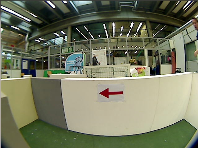
In order to reduce the time required to finish the maze, we use the arrows that are placed around the maze to guide us towards the exit. To recognize the arrows we use the camera mounted on Pico, but the raw footage (displayed below) needs to be processed in order for Pico to detect arrows. | |||
[[File:Camera_Original.jpg|center|The original camera image in RGB values]] | |||
=== Initial Cropping === | |||
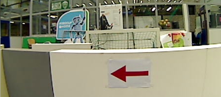
We start of by cropping the initial RGB image, because we do not need to detect an arrow in the whole image, only in the center. This reduces the calculation time as well as the disturbances from the environment. The cropped image is showed below. | |||
[[File:Initial_Crop.jpg|center|The first crop of the original image]] | |||
=== Template Matching === | |||
Then we use Template Matching to give a good first estimate of where the arrow is. We use both a right and left arrow template to run over the image, where the following formula returns a value for the similarity between the template and the actual image at every pixel: | |||
<math>R(x,y) = \sum_{x',y'} (T(x',y')-I(x+x',y+y'))^2 </math> | |||
The pixel with the lowest value gives us the best estimate of where the arrow is. We then crop the image even further, it is now the size of the template. We also already have an idea if the arrow is towards the right or left, since the template matching function of the correct arrow will have returned the lowest value. The cropped image is displayed below. | |||
[[File:Template_Crop.jpg|center|The second crop of the original image, using the template match]] | |||
=== Thresholding === | |||
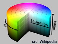
Next, the small image (which still has RGB values), is converted to the HSV color space. We then perform thresholding for the following values (HSV(165-179,240-255,100-175) and HSV(0-20,240-255,100-175)), in order to seperate the red in the (RGB) image from everything else. The resulting binary image is white where the original RGB image was red and black for any other color. Note: we use two seperate thresholds to create two binary image, which we subsequently combine, because red is exactly at the end of the spectrum in the HSV values in OpenCV. This means that red can have the value of H = 0, as well as H = 179, which can be seen in the picture to the right of the HSV Cylinder. The seperate binary images as well as the combined one are displayed below (we use a right arrow because this one demonstrates the use of two thresholds the best). | |||
[[File:hsvColorCylinder.jpg|thumb|right|HSV Cylinder]] | |||
[[File:Binary1.jpg|center|HSV(165-179,240-255,100-175)]][[File:Binary2.jpg|center|HSV(0-20,240-255,100-175)]][[File:Binary.jpg|center|Combined (final) binary image]] | |||
=== Dilating and Eroding (Closing) === | |||
Because this binary image is still very noisy and the arrow is not completely filled, we use two iterations of dilating followed by two iterations of eroding the image. Dilation consists of convoluting an image with a certain kernel of any shape or size. The kernel has an anchor point, which usually is in its center. As the kernel is run over the image, the maximum pixel value overlapped by the kernel is determined, and the pixel of the image in the anchor position of the kernel gets that maximum value. This makes the bright areas in the image become larger, which in our case is the arrow. Erosion is very similar, only that instead of the maximum pixel value, we take the minimal pixal value above. This makes the dark areas bigger, thus reducing the size of the arrow. We use a rectangular kernel of size 4 for the dilation as well as the eroding. The process of dilation followed by eroding is also called closing an image. The result is an arrow with its gaps filled and the rough edges smoothened out, as displayed below. | |||
[[File:Dilated_and_Eroded.jpg|center|Closed Image]] | |||
=== Edge Detection === | |||
Now that we have a clear binary image of the arrow we are driving towards, we first calculate its center by checking the pixel that is on the far left and the pixel that is on the far right which are both still white. We will use this later on. | |||
Then we use the binary image to detect the edges of the arrow. This is done by using the 'Canny Edge Detector', which detect the lines by checking the gradient of the pixels. The result is in the picture below. | |||
[[File:Edges.jpg|center|Edges]] | |||
=== Hough Transform === | |||
Now that we have detect the edges of the arrow, we want to define the lines where the edge consists of. For this we use the Hough Transform. This algorithm calculates for every pixel in the image all the lines that can pass through this point, in polar coordinates. We take a resolution of 1 pixel and 1 degree for the distance and angle respectively. If two (or more) pixels have the same value for the distance and angle, this means they belong to the same line. We use a threshold of 50 pixels that should have the same polar values before we consider it to be a line. We us the probabilistic Hough Transform, which is a more efficient algorithm than the standard Hough Transform. Then we check if two of the detected lines are in the correct angle to form the point of the arrow, and on which side of the center (calculated before) they are. If they are to the right of the center, we expect it to be a right arrow. The result of the line detection is below, together with the center line in blue. | |||
[[File:HoughLines.jpg|center|Lines]] | |||
=== Corner Detection === | |||
The final image process step is to determine corners in the image. For this, we use the OpenCV function 'goodFeaturesToTrack'. It uses the minimal eigenvalues of gradient matrices to detect corners and removes corners which have an eigenvalue lower than the quality level specified. Also, it compares the remaining corners to the other corners detected, and if there are corners at a distance smaller than the max distance specified, it chooses the corner with the strongest quality measure. Then we check if where the most corners are detected (left or right of the center) and the side which has the most corners is most likely to be where the arrow is pointing. The detected corners together with the center line are shown in the picture below. | |||
[[File:Corners.jpg|center|Corners]] | |||
=== Summary Arrow Detection === | |||
In conclusion, we use three checks to determine if there is an arrow and which way it is pointing: | |||
1. By using the template matching and checking if the left or right has the best score | |||
2. By checking the lines and to see if there are two lines at about plus and minus 30 degree angles and at which side of the center they are | |||
3. By detecting the corners and checking on which side of the center the most are located. | |||
Finally we also iterate over three correct detections in a row to make absolutely sure an arrow is correctly detected. This process is shown in action in the video below, | |||
[[File:cameraVideo.jpg|left|link=http://www.youtube.com/watch?v=ZlOCnwAHsJk]] | |||
'''* http://www.youtube.com/watch?v=ZlOCnwAHsJk''' | |||
<br /> | |||
=== Possible Improvements === | |||
- Use smoothing on original image to reduce noise. (If your goals is to have a binarized image with smooth edges then, if you have the original, it is better to use something like a gaussian blur with cvSmooth() on that before performing the binarization.) (http://stackoverflow.com/questions/5154282/dilate-erode-modify-kernel-option) | |||
- blur before edge detection | |||
- different dilating/eroding, maybe circle for dilating and rectangle for eroding? | |||
- different kernel size for closing, blurring, edge detection and everything. | |||
=== Sources === | |||
- http://en.wikipedia.org/wiki/HSL_and_HSV | |||
- http://docs.opencv.org/doc/tutorials/imgproc/erosion_dilatation/erosion_dilatation.html | |||
- http://docs.opencv.org/doc/tutorials/imgproc/opening_closing_hats/opening_closing_hats.html | |||
- http://stackoverflow.com/questions/5154282/dilate-erode-modify-kernel-option | |||
== Filtering and Processing Laser Data == | |||
''20 Sept 2013'' | ''20 Sept 2013'' | ||
| Line 220: | Line 352: | ||
After visualizing the environment as we wanted to; we now focus more on tasks of the robot as some of the tasks have to be carried out at all times (e.g. obstacle avoidance) and others have to be completed upon requests (e.g. change in trajectory due to decision making). | After visualizing the environment as we wanted to; we now focus more on tasks of the robot as some of the tasks have to be carried out at all times (e.g. obstacle avoidance) and others have to be completed upon requests (e.g. change in trajectory due to decision making). | ||
== Laser data visualized == | |||
''18 Sept 2013'' | ''18 Sept 2013'' | ||
| Line 228: | Line 360: | ||
[[File:Cartesian.gif]] | [[File:Cartesian.gif]] | ||
== ROS Nodes and Topics== | |||
''17 Sept 2013'' | ''17 Sept 2013'' | ||
Latest revision as of 20:54, 18 July 2016
Group Members
| Name: | Student id: | Email: |
| Justin Wildschut | 0617495 | j.a.wildschut@student.tue.nl |
| Jeroen Zegers | 0638172 | j.c.zegers@student.tue.nl |
| Alex Andriën | 0652965 | a.r.p.andrien@student.tue.nl |
| Talha Ali Arslan | 0867550 | t.a.arslan@student.tue.nl |
| Leroy Hazeleger | 0651762 | l.hazeleger@student.tue.nl |
Maze challenge evaluation
The program used to successfully find the exit of a maze was insufficient. The robot entered the first crossing where it encountered a small pocket left and right of the path. Since the pockets left and right where very small, it should go straight since the program neglects pockets which are not useful to explore. Thus the robot continued and wanted to exit the first crossing but it stopped moving when it wanted to exit the crossing. Normally this should not happen. For driving out of the crossing there are three different states where it can be in. Somehow, at first it entered the first state where it follows the right minimum to position itself into the path, after that it changed state (which should not be possible) and this resulted in the fact that it lost its current state and the robot just stopped. Of course in the second trial the same problem should occur, and it did. The day before the maze challenge we added another if() statement which caused this problem and we knew it before the second trial, but we thought that we could not change the code between the two trials.
When the challenge was finished, we did a third trial, of the records, were we erased that extra if() statement. After that, the robot was able to continue, detected both the arrows but at the end it did not go to the exit unfortunately....
Discussion and Possible Solutions
* http://www.youtube.com/watch?v=MNNZ6KVImGg
Program Structure
Already before the corridor challenge we divided the program into nodes. We did this because the code we wrote for the corridor challenge became very large and it was hard to keep the overview of the code. Furthermore we realized that if we divide the code into parts we can split responsibilities easier. In the end the total program was divided into the nodes as shown below. The division of the program into these nodes helped us a lot because everyone had the overview of the function of each block and it was easier to debug the entire code. We documented the message types of the topics between the nodes and we described the function of each node.
The whole ´pipeline´ is updated on a rate of 40Hz, every time a new laserdata frame is received all the callback functions are called and the processed data or decisions are published. It is of no use to update the pipeline with a higher rate than 40Hz because the data is not refreshed with a higher rate. With the pipeline all nodes are meant except for the camera node. The camera node works with a refresh rate of 30Hz, the update rate of the camera on the jazz robot.
Because the refresh rate of the pipeline is 40Hz the calculation time of each node is limited. Each node has a maximum of 1/40th of a second to publish the processed data and read the new data from the buffer. If the nodes would use more time the buffers in ROS would overflow and data will be lost resulting in inaccuracy and errors. Because the CPU used is so powerful the most expensive calculation in the pipeline is (only) processing a 1080 byte vector the limited time is not a problem. Furthermore, the splitting of the program in nodes assures the time limit will not be reached. The only time crucial node would be the Camera node. But because the camera refreshes on another rate and so the Camera node is not a link in the pipeline this is no problem either.
In the beginning there was some doubt whether the structure would not introduce too much delay. The delay introduced by the whole pipeline proved to be negligible. All nodes introduce a delay of one frame, except for the Averaging node, this one introduces 3 frames of delay because it takes the average of three laserdata frames. The total delay is 8 frames which corresponds to .2 seconds and an approximate distance of 4cm at a velocity of .2m/s.
All nodes have a specific function which is described below. As is depicted in the program structure there is a node called Mapper. The mapper is implemented as a function in the node Decision Making but can be seen as a node. Implementing the Mapper as a function proved to be more convenient and gave us more freedom considering the data generated in this node is needed in the algorithm of Decision Making.
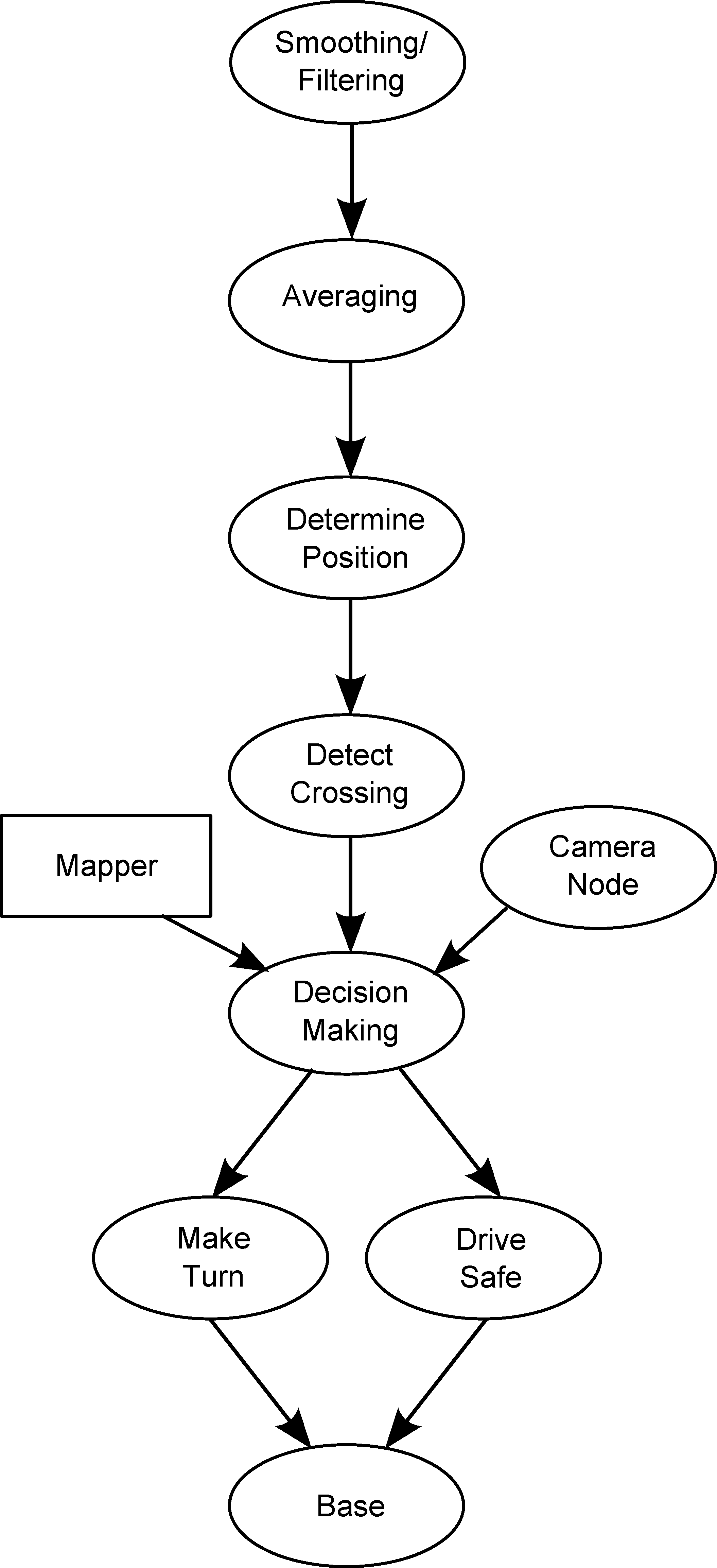
The nodes and topics are described in the following document: File:EMC Main.pdf
Smoothing Node
Here, the raw laser data is smoothened using a moving average. This is done by averaging each value from the laserscanner with its neighbours, which leads to data with less noise in it, which is sent to the Averaging node.
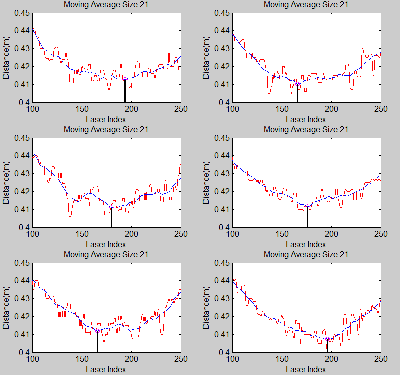
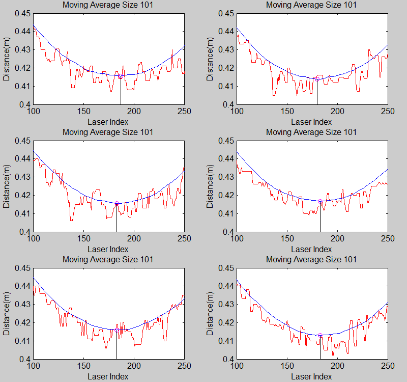
The smoothing is done by applying the moving average method in a variable window size. In this method, moving average at every index is calculated by taking the sum of 'window size' number of elements to the left and right (combined) of that point and dividing it by the window size (i.e. if the window size is 21, 10 points to the back, 10 points to the front and the current point is taken into account). We first started with a constant window size, but there were problems. Because the resolution of laser readings is high over small portions at close distances and low over large portions at large distances, we had to adjust the moving average window size accordingly. In these gifs on the upper left and center, you will see what happens if we use a small and large window size at close distances (Look at with small window size how the minima index changes rapidly and how smoothened the data is, and at large window size, look at how the data is smoothened and there not that much rapid change in minima location as with smaller window size, but there is still movement and this will be overcome in the next node 'Averaging Node').
One of the first assumptions was that the laser data below a magnitude of 0.15 m is due to the body of the robot. This is only correct for large distances. In the simulation this holds everywhere but in the real world, we discovered that at close distances first indices of the laser read distances 'between' the actual distance and 0; they look like an interpolation between 0 and those distances and we do not know why this happens; we guess that it may be due to the white shiny surface of the robot case that beams can reflect and be effective at close distances or it may just be a bug of the laser. So; because we depend our smoothing of laser data and determination of local minimum and maximum distances based on these start and finish indices, we should no longer use a dynamic start index and based on real world testing, we should constantly avoid first and last (~approximately) 20 indices which are around 18 in the simulation. We can increase these values based on readings (if a reading below 0.15m still comes after 20th index, we may shift starting index to that value but it should never be below 20). This gif file on the upper right shows the phenomena; where at first the distance to the wall is close, and when the distance increases the problematic readings goes below the line of 0.15 m (black) which was our previous assumption.
The gif pictures below show the whole data and the effect of window size on smoothing. Basically it is seen that with small window size, the smoothened data resembles the original more (not oversmoothened) but at close distances location changes too rapidly and even multiple maximas are found close to each other in some instances. Using a larger window size gives advantage at close distances and flat surfaces, but you can see in the middle gif that data is over smoothened and some corners to the sides are dislocated too much. Below right show a dynamical window result, at distances above a certain distance constand window size is used but between a preferred distance region, window size is proportionally changed between 21 and 101 in this case. Using a very large window size is also not preferable because it increases computation time. Because we use dynamical window, we cannot use a moving array which would solve that problem actually.
How the local minimum values are found is explained in the 'DeterminePosition Node' part.
Averaging Node
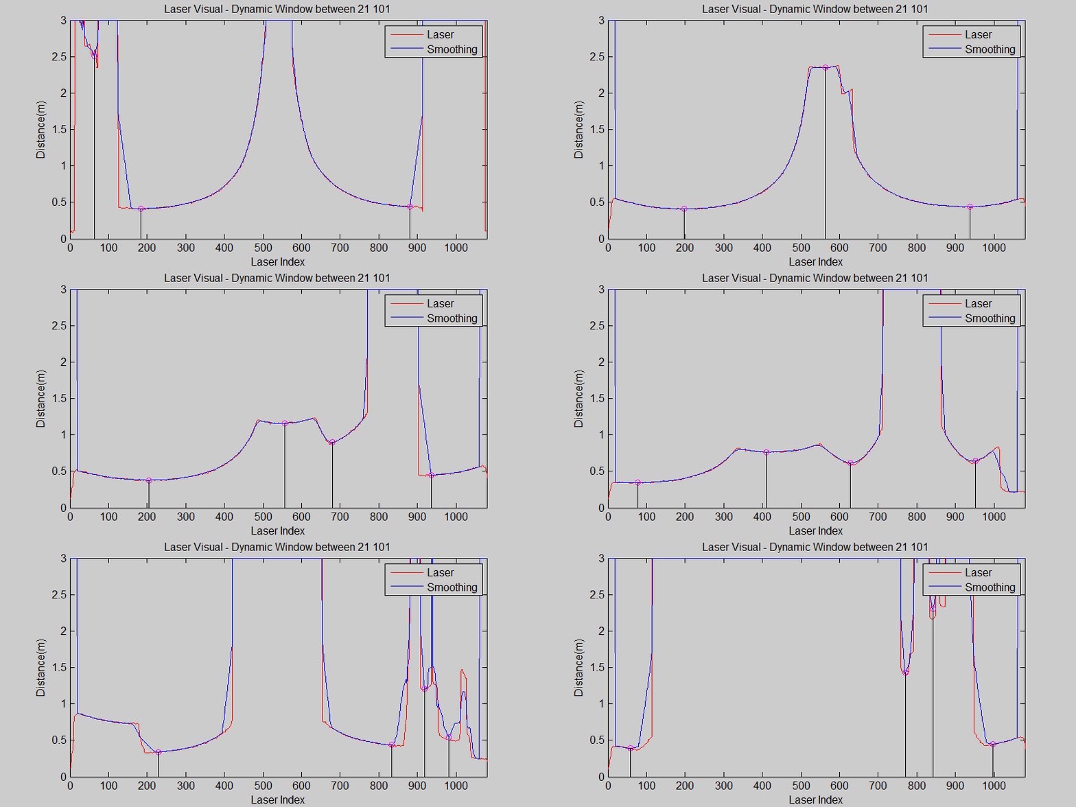
In contrary to the Smoothing node, which averages over all the laser data from a single time instance, this node averages the already smoothened data over several time steps. This is necessary because if there is a disturbance in a single timestep (a large dust particle in front of the laser for instance), we don't want the program to detect things that aren't there. The Averaging reduces the effect of such disturbances. The smoothened, averaged data is then sent to the Determine Position node.
In the visuals above, one can see that averaging helps reduce the oscillation of the minimas.
Determine Position Node
Here, the smoothened and averaged data is analysed. The minima and maxima of the laser data are determined, as well as their corresponding indices. This data is sent to the Detect Crossing node.
In this node, every data point from the Averaging node is checked according to its distance and index, relative to the other points within a constant window, where the current point is in the center. Also local maximas or minimas next to each other who have same distances are avoided and only one is taken into account, because from the smoothened and averaged data, there can be points next to or close to each other with same distance value.
Result of this node can be seen in the gif pictures in 'Smoothing Node' and 'Averaging Node' where local minimas are plotted with a circle and a vertical line.
Detect Crossing Node
As is presented in the program structure above there is a node which detects the crossings/intersections in the maze. This node detects at which moment PICO is at the middle of a intersection and if there is a side-path on its left and/or right and/or a path in front.
Detection of an intersection
The different types of intersections are detected using a search algorithm. It will look for certain combinations of minima at certain angles. The positions of these local minima are found in the 'Determine Position' node and send via a topic to this 'Detect Crossing' node. The local minima which are found by the 'Determine Position' node will be filtered using a certain treshold. Only the minima which are relatively close to the robot are of interest for detection of the intersections. This treshold depends on the pathwidth which is determined using the laserdata. For example, the four-way-intersection which is the first intersection displayed in the figure below is detected using the two minima of the corners in front. The angle between these minima should be approximately 90 degrees and both minima should be at an angle of approximately 45 degrees with the centerline of the path in which the robot is driving. If the robots pointing direction is not parallel with the centerline of the path the angles at which the detection node searches for the minima is adapted accordingly. Since the minima cannot be detected perfectly and since the angular position of the robot cannot be estimated perfectly a detection region is used for detecting these minima. This detection region is illustrated by the green lines in the figures and the width of this detection region is two times delta. With delta being a tuned parameter which was set on 15 laserscanner data increments. Since there are multiple types of intersections, the node searches for different combination of minima at certain angles at the same time when it is driving through a corridor. The types of intersection which can be detected and the according combination of minima are displayed in the figure below.
Above is explained how the different types of intersections are detected when PICO is driving through a corridor. The Detection node communicates to the DecisionMaking node, which is decribed later on, that it is at the approximate middle of an intersection and which options there are to take; go left, go right, go straight and/or turn around.
Detect when a turn is made
When the Decision Making node decides to go straight on it is not necessary to make a turn and the Drive Safe node, which will be elaborated further on, will be activated directly and PICO continues its way in the same direction. If the Decision Making node decides to make a turn, the Make Turn node is activated and PICO starts to turn. The Detect Crossing node looks if there is a single minimum at a certain detection region while PICO is turning (see images in the figure below). Note that for the dead-end "intersection" the algorithm will look for two opposite minima instead of only one minima at a certain angle. The detection algorithm will search for this single minimum at any time however this information will only be used in the Decision Making node when the robot is making a turn. Let's continue with the example described above, PICO is at the approximate middle of a four-way-crossing and the DecisionMaking node decides to make a left turn. Then the robot will start to turn left untill another minimum is at an angle of 45 degrees in clockwise direction w.r.t. the robots pointing direction. This situation is illustrated in the most upper left image of the figure below. The other images illustrate the detection of a (different) single minimum which indicate that the particular turn is made. Note that the detection of when to stop turning is always done using one minimum which is also used to detect the intersection itself. In this way varying pathwidths will not cause any problems during turning, which is described more elaborately in the last section of this chapter.
Early dead-end detection
When the detection algorithm detects a certain type of intersection it will also look for possible (short) dead-end corridors. Suppose the robot is at the approximate middle of the intersection displayed in the left image of the figure below. Without the early dead-end detection the Detect Crossing node would detect the intersection as a four-way-crossing using the two minima within the green detection regions. However, an early dead-end detection algorithm is included in the detection node. When PICO is at an approximate center of an intersection, the early dead-end detection checks if there are minima within a certain distance in possible side/front paths. These regions of detection are illustrated by the orange lines. If a minimum within a close distance is detected in a possible side or front corridor, PICO will not see this short dead-end as a possible way to go. Thus the detection algorithm will see the intersection depicted in the left image in the figure below as an intersection with only a path to the left (this is illustrated using the dashed red lines). Thus the only option which the Decision Making node will have is to turn left. The right image in the picture below shows another example of early dead-end detection.
Robustness for variable pathwidth within a maze
Since the pathwidth within the maze was not known beforehand it was necessary to implement some adaptation into the program. We tried to design our program in a way such that it can handle various pathwidths. It was communicated to us that the pathwidth within the maze could vary with +/- 15 centimeter, therefore we also thought about how to cope with these pathwidth differences. In the figures shown above is shown that the detection still works even if the pathwidths of the corridors within the maze differ for 20 centimeter or even more. This is also shown using the figure below. The dashed grey lines indicate the centerline of a corridor . If the robot is driving through a corridor it will approximately follow the centerline of this particular corridor . When the intersection is detected and a turn is made, using the method described earlier on in this chapter, the robot is not at the centerline of the corridor which it will enter. However this is no problem since the Drive Safe node will correct for this while driving into this corridor, which is described in the chapter about the Drive Safe node.
To see the crossing detection in action see the link below. The different pathwidths are illustrated in the figure below.
Decision Making Node (UNDER CONSTRUCTION)
The Decision Making node is the connecting node of the whole structure, in other programs called the 'brains' or 'master' node. This node contains the strategy to solve the maze and uses the Camera arrow detection and info stored in the Mapper to find the fastest way out of the maze. As depicted the program is state-based. There are four main states; Drive Safe, Drive Straight, Make Turn and Turn Around.
When the Decision Making is in the states Drive Safe or Drive Straight the Drive Safe node is activated. In the state Drive Safe the robot is driving in between two walls. The Decision Making sends a '1' to the Drive Safe node and a '0' to the Make Turn node. The Decision Making leaves this state when a crossing (including dead-end) is detected. In this state the Drive Safe node orientates on the minima on the sides of the robot.
In the state Drive Straight the Decision Making node sends a '2' to the Drive Safe node and a '0' to the Make Turn node. By sending a '2' to the Drive Safe node the node orientates using the correct minima for each crossing.
In both Drive-states the robot has mostly linear velocity and all angular velocity is controlled by the Drive Safe node. When the Drive Safe node receives a '0' it will stop publishing on the base control topic.
When the Decision Making is in the states Making Turn or Turning Around the node sends a '1' or '2' to the Making Turn and a '0' to Drive Safe. The value sent determines the direction the robot will turn. This means that the robot has only angular velocity and turns on it's base. The Decision Making node leaves the Making Turn state when Detect Crossing detects the correct crossing.
The state Turning Around is developed especially for when the robot encounters a dead-end. The robot needs to turn 180 degrees and during turning two particular situations must occur subsequently before the robot is turned completely. The crossing type published by the Detect Crossing should change twice, first to 'Right' and then to 'Straight'.
Mapper
To see the mapper node in action:
It is easy to remember which turns robot has made over time and to manipulate its choices by always making a specific turn or balancing them. However the task of remembering where it has come from and what choices remain is rather complex. For this we tried to simplify the problem as much as possible. At every new node, a term is added to the map which is kept as an [some constant][node count] size array. When the robot crosses a node, map is updated on that node, so that when the robot comes back, it knows which direction it has come from, where it can go and cannot go. When a dead end is reached, it reflects back on previous nodes too and as robot makes its way back to the last node where there is an option to go to, nodes are erased from the array. So, in the end, if the robot makes it out of the maze, we have an array with smallest amounts of nodes in it, and with 'dead end' information in them.
Every node is defined as 4 term vector:
[current , right of the current , ahead of the current , left of the current]
It is simply a record of ways in counterclockwise directions. The term current 'Current' is where the robot is and it can either be 3 or 4 (4 means that there is a dead end behind the robot and it is returning). Other terms can be 0,1,2,4. 0 means there is no opening (wall). 1 means it is an option that is not discovered yet. 2 means robot has come from there before. 4 means there is an opening but it has dead end(s).
As an example 'T crossing' is defined as [3101]. Current direction is 3, the one to the right is 1 (there is an opening), ahead is 0 (wall), left is 1 (there is an opening too). As another example, a right corner is defined as [3100] or a left corner [3001] or when the robot drives between walls [3010] (but this is not added to the map other than the start). If there is a 4-way crossing it is [3111].
If the robot crossed a new right corner, it first detects it as [3100] and when it makes the turn and passes it, map updates that term to be [3002]; because now it has become a left turn. Same with if the robot makes a left turn at a 4-way crossing [3111] after the node is passed, that node will be updated as (it turned left so now it is as if it has come from the right), [3211]. Take for instance the node type of [3110] where the robot can continue straight or right and there is no opening on its left. If it makes the right turn, (if it comes back to that node) the wall will be at its front, the option that it did not go before will be on its right and its previous choice will be on its left; [3102]. When the robot gets to dead ends, it updates current 3 as 4 and this effects previous nodes too. As an example at an 4 way crossing in the maze at the very start, we assume for the maze competition that on of them can be the correct one. Initially it will be [3111] and if we are not so lucky, we are going to eliminate all the dead ends and the node will become for example [4241]. 2 is where the start of the maze is (on the right) and this means that if we chose the option straight ahead at first it could have saved us time.
So discovering the maze requires a strategy of choosing between the undiscovered options, but returning from dead ends requires only remembering the nodes and making our way back to a desired node correctly.
Drive Safe Node
The Drive Safe node makes sure that PICO drives safely throughout the whole maze. This means that PICO drives safely between walls so that it does not hit a wall and drives optimally through the pathway, it detects when it is entering a crossing and drives safely and straight to the middle of the crossing, and after PICO made the correct turn it exits the crossing safely and straight. After it exits the crossing, it continues to drive safely between walls.
The Drive Safe node is divided into four states: Normal Driving, Enter Crossing, Exit Crossing and Safety Driving. The Decision Making node determines if the Drive Safe node should be in the Normal Driving state,in the Exit Crossing state or PICO should do nothing. It publishes a Drive message of 1 if PICO should drive safely between walls (Normal Driving state), publishes a Drive message of 2 if PICO exits a crossing (Exit Crossing state) or publishes a Drive message of 0 if PICO should stop moving so that a turn can be made. Within the Drive Safe node, it is determined if PICO is actually between walls (Normal Driving state, Drive message 1), enters a crossing (Enter Crossing state, Drive message 1) or perform a ` special' maneuver to prevent collision (Safety Driving, Drive message 1). To determine the state in which PICO is, the message published by the Determine Position node is used which tells us where the minimum distances to the wall are located (index between 0 - 1081) and provides the distance to that minimum. Since we are interested only in the local minima, i.e. minima below a certain threshold, only the minimum distances below the threshold are considered in the Drive Safe node. Below, the different parts are explained in more detail.
Note that all thresholds are tuned during the real-time experiments
Normal Driving
PICO is in the `Normal Driving' mode if PICO is located between walls. In order for PICO to take the turns correctly, PICO should remain approximately in the middle of the path with its forward position parallel to the walls before it will be in the `Enter Crossing' mode. To determine when PICO is located between walls, we know that there are at least two minima which are approximately 180 degrees apart (approximately since the noise disturbs the Determine Position node). If those two minima are indeed approximately 180 degrees apart PICO is between walls, and if this is not the case (the angle between the two minima differs to much with a certain threshold) PICO enters a crossing. Also if one of the minima becomes to small, PICO goes into the Safety Driving node.
The two minima (index and distance, indicated by the red lines) are used to determine the width of the path (orange line), the position from the middle of the path (difference between the green and blue line, left from the blue line is negative) and the angle between the forward position and the right wall and the left wall (purple lines). Those are depicted in the figure below.
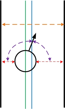
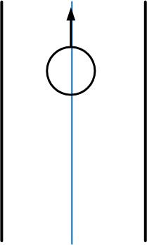
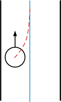
The width of the path is determined by summation of the distances of the two minima.
[math]\displaystyle{ \frac{}{}widthPath = distance_{left} + distance_{right} }[/math]
The position from the middle of the path is determined by dividing the width of the path by 2 and subtracting the distance to the right minimum.
[math]\displaystyle{ posFromMiddle = \frac{widthPath}{2} - distance_{right} }[/math]
Using the minimum angle and the angle increment, the angles of the two minima [math]\displaystyle{ \theta_{left} }[/math] and [math]\displaystyle{ \theta_{right} }[/math] are determined.
What we want is that PICO drives in the middle of the path and if not, it drives optimally to the middle of the path. Therefore we would like PICO to drive to the middle of the path by following a exponential decay towards to middle of the path. The exponent decay is shown by the red line in the figure above.
[math]\displaystyle{ \frac{}{}posFromMiddle(t) = posFromMiddle_{int} * e^{\beta t} }[/math]
Since we can only control the linear and angular velocity, the slope of the exponent in each point is determined
[math]\displaystyle{ \frac{d}{dt}posFromMiddle(t) = \beta * posFromMiddle_{int} * e^{\beta t} }[/math]
and from this exponent the desired netto angle of PICO is determined.
[math]\displaystyle{ \theta_{desired} = sin(\frac{\beta*posFromMiddle}{\sqrt{1+\beta^2*posFromMiddle^2}}) }[/math]
The actual netto angle is determined using the following equation
[math]\displaystyle{ nettoAngle = \frac{\theta_{left} + \theta_{right}}{2} }[/math]
The angular velocity is then calculated is the actual netto angle minus this desired netto angle and multiplied with a constant, resulting in an exponential decay towards the middle of the path.
[math]\displaystyle{ \frac{d}{dt}\theta_{z} = constant*(nettoAngle - nettoAngleDesired) }[/math]
Of course [math]\displaystyle{ \beta }[/math] can be chosen very high so that PICO returns quickly to the middle of the path, however from real-time experiments was observed that PICO has an overshoot due to a certain delay. Therefore [math]\displaystyle{ \beta }[/math] and the constant are tuned so that PICO moves to the middle of the path without oscillating around the middle.
Entering Crossing
When the two minima do not make an angle of approximately 180 degrees and PICO was in the Normal Driving state before, PICO enters a crossing. From the location of the different minima that are observed can be determined what type of crossing it enters.
T-crossing, left turn or right turn
If there is one minimum detected approximately at index 540 (within the threshold of course), we know that there is a wall in front of PICO. The only thing we want is that PICO drives towards this minimum so that drives straight into the crossing and can detect a crossing accurately using the DetectCrossing node. So the angular velocity is adapted so that the minimum will be detected around index 540 the whole time. The figures below show the different crossing when it should go to the minimum at index 540. So we correct the angle of PICO, for instance if the minima is at index 580, we know that PICO is oriented to the left, and we give it an angular velocity to the right.

Left turn or right turn with a straight path
If there is no minimum approximately at index 540, and if there is one minimum detected approximately at index 180 (right), or one minimum detected approximately at index 900 (left) and not both at the same time of course otherwise we are between walls, then we know that PICO enters a crossing where you can turn right or straight and respectively left or straight. Since the width of the path can not be measured in the crossing, the old width of the path is remembered and the same strategy is used as in the Normal Driving state to drive to the middle of the path and to drive straight with respect to the wall (right or left).
Three-way crossing
If the T-crossing, left turn, right turn, left turn or right turn with a straight path do not occur, then PICO enters a three-way crossing. Now we need to use the two minima which are in front of PICO but the number of minima can vary between 2, 3 or 4 minima in the threshold. Also the index of two minima in front of PICO will change when PICO enters the crossing. Therefore, depending on the number of minima in the threshold, the right minima are selected and the angular velocity is changed such that the distances to these minima become equal. So if the left minima of the two is further away than the right minima, then PICO should be oriented to the left and should drive forward.
Exiting Crossing
When PICO is entering a crossing, a Drive message of 1 is published by the Decision Making node. At a certain point, the Detect Crossing node detects a crossing and the Decision Making node publishes a Drive message of 0 and PICO is will make a turn accordingly. During the Drive message of 0, PICO does not drive, and only turns. When the turn is finished, a new Drive message of 2 is published by the Decision Node and PICO is in the Exit Crossing state.
In the Exit Crossing state, the same method as in the Enter Crossing state could have been applied. However the problem with that is that when PICO turns, the width of the new path it will enter can be different from the path it came from and is unknown. Also the position from the middle is unknown and therefore the algorithm as used previously cannot be used. It can only be used if it is guaranteed that the width of the new path is equal to the old width of the path.
When PICO made the turn, three different situations can occur: a left + straight crossing can be seen, a right + straight crossing can be seen, or a three-way crossing can be seen. These are given in the figures below. The Detect Crossing node made sure that PICO stopped in approximately the middle of the intersection. Therefore what we like to have is that PICO moves straight into the new path, but due to the turn it made, the back wheels are orientated perpendicular to the new driving direction. Therefore we need a new control strategy which corrects PICO if it does not move straight into the new path. Depending on the minima it detects, the different situations occur and have different strategies. If a left + straight crossing can be seen when PICO made a left turn, PICO should follow the right wall since at index 180 a minimum will be seen. By keeping the index of this minimum at index 180 PICO can move straight into the new path. If the minimum is detected at for instance index 200, PICO is oriented in the direction of the right wall and the angular velocity should be positive. When there are two minima within the theshold which are 180 degrees across each other, then PICO is in the path ,thus PICO is between walls and a Drive message of 1 is published by the Decision Making node. PICO can continue in the Normal Driving state.
The same strategy is used for the right + straight crossing, which can seen when PICO made a right turn before. A minimum at approximately index 900 can be seen and should stay at index 900.
For the three-way crossing the same strategy as in the Enter Crossing state is used: A minimum at approximately index 360 and a minimum at approximately index 720 can be seen, and those distances are kept equal by adjusting the angular velocity. Those minima will change index, but rather than looking for the minima at those indexes, it is checked what the indexes are of those two minima.
Safety Driving
When PICO is too close to a wall, PICO should stop driving forward to prevent collision. Thus if the minimum distance is closer then 30 cm, then PICO stops driving forward and backs up till the minimum distance is 45 cm. After that, PICO can continue to drive safe; in drive safe the orientation of PICO will be corrected and therefore PICO will not come close to a wall.
Camera Node
In order to reduce the time required to finish the maze, we use the arrows that are placed around the maze to guide us towards the exit. To recognize the arrows we use the camera mounted on Pico, but the raw footage (displayed below) needs to be processed in order for Pico to detect arrows.
Initial Cropping
We start of by cropping the initial RGB image, because we do not need to detect an arrow in the whole image, only in the center. This reduces the calculation time as well as the disturbances from the environment. The cropped image is showed below.
Template Matching
Then we use Template Matching to give a good first estimate of where the arrow is. We use both a right and left arrow template to run over the image, where the following formula returns a value for the similarity between the template and the actual image at every pixel:
[math]\displaystyle{ R(x,y) = \sum_{x',y'} (T(x',y')-I(x+x',y+y'))^2 }[/math]
The pixel with the lowest value gives us the best estimate of where the arrow is. We then crop the image even further, it is now the size of the template. We also already have an idea if the arrow is towards the right or left, since the template matching function of the correct arrow will have returned the lowest value. The cropped image is displayed below.

Thresholding
Next, the small image (which still has RGB values), is converted to the HSV color space. We then perform thresholding for the following values (HSV(165-179,240-255,100-175) and HSV(0-20,240-255,100-175)), in order to seperate the red in the (RGB) image from everything else. The resulting binary image is white where the original RGB image was red and black for any other color. Note: we use two seperate thresholds to create two binary image, which we subsequently combine, because red is exactly at the end of the spectrum in the HSV values in OpenCV. This means that red can have the value of H = 0, as well as H = 179, which can be seen in the picture to the right of the HSV Cylinder. The seperate binary images as well as the combined one are displayed below (we use a right arrow because this one demonstrates the use of two thresholds the best).


Dilating and Eroding (Closing)
Because this binary image is still very noisy and the arrow is not completely filled, we use two iterations of dilating followed by two iterations of eroding the image. Dilation consists of convoluting an image with a certain kernel of any shape or size. The kernel has an anchor point, which usually is in its center. As the kernel is run over the image, the maximum pixel value overlapped by the kernel is determined, and the pixel of the image in the anchor position of the kernel gets that maximum value. This makes the bright areas in the image become larger, which in our case is the arrow. Erosion is very similar, only that instead of the maximum pixel value, we take the minimal pixal value above. This makes the dark areas bigger, thus reducing the size of the arrow. We use a rectangular kernel of size 4 for the dilation as well as the eroding. The process of dilation followed by eroding is also called closing an image. The result is an arrow with its gaps filled and the rough edges smoothened out, as displayed below.

Edge Detection
Now that we have a clear binary image of the arrow we are driving towards, we first calculate its center by checking the pixel that is on the far left and the pixel that is on the far right which are both still white. We will use this later on.
Then we use the binary image to detect the edges of the arrow. This is done by using the 'Canny Edge Detector', which detect the lines by checking the gradient of the pixels. The result is in the picture below.

Hough Transform
Now that we have detect the edges of the arrow, we want to define the lines where the edge consists of. For this we use the Hough Transform. This algorithm calculates for every pixel in the image all the lines that can pass through this point, in polar coordinates. We take a resolution of 1 pixel and 1 degree for the distance and angle respectively. If two (or more) pixels have the same value for the distance and angle, this means they belong to the same line. We use a threshold of 50 pixels that should have the same polar values before we consider it to be a line. We us the probabilistic Hough Transform, which is a more efficient algorithm than the standard Hough Transform. Then we check if two of the detected lines are in the correct angle to form the point of the arrow, and on which side of the center (calculated before) they are. If they are to the right of the center, we expect it to be a right arrow. The result of the line detection is below, together with the center line in blue.

Corner Detection
The final image process step is to determine corners in the image. For this, we use the OpenCV function 'goodFeaturesToTrack'. It uses the minimal eigenvalues of gradient matrices to detect corners and removes corners which have an eigenvalue lower than the quality level specified. Also, it compares the remaining corners to the other corners detected, and if there are corners at a distance smaller than the max distance specified, it chooses the corner with the strongest quality measure. Then we check if where the most corners are detected (left or right of the center) and the side which has the most corners is most likely to be where the arrow is pointing. The detected corners together with the center line are shown in the picture below.

Summary Arrow Detection
In conclusion, we use three checks to determine if there is an arrow and which way it is pointing:
1. By using the template matching and checking if the left or right has the best score 2. By checking the lines and to see if there are two lines at about plus and minus 30 degree angles and at which side of the center they are 3. By detecting the corners and checking on which side of the center the most are located.
Finally we also iterate over three correct detections in a row to make absolutely sure an arrow is correctly detected. This process is shown in action in the video below,
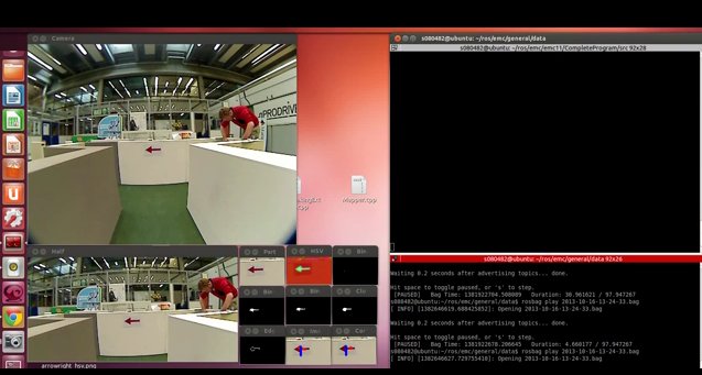
* http://www.youtube.com/watch?v=ZlOCnwAHsJk
Possible Improvements
- Use smoothing on original image to reduce noise. (If your goals is to have a binarized image with smooth edges then, if you have the original, it is better to use something like a gaussian blur with cvSmooth() on that before performing the binarization.) (http://stackoverflow.com/questions/5154282/dilate-erode-modify-kernel-option)
- blur before edge detection
- different dilating/eroding, maybe circle for dilating and rectangle for eroding?
- different kernel size for closing, blurring, edge detection and everything.
Sources
- http://en.wikipedia.org/wiki/HSL_and_HSV - http://docs.opencv.org/doc/tutorials/imgproc/erosion_dilatation/erosion_dilatation.html - http://docs.opencv.org/doc/tutorials/imgproc/opening_closing_hats/opening_closing_hats.html - http://stackoverflow.com/questions/5154282/dilate-erode-modify-kernel-option
Filtering and Processing Laser Data
20 Sept 2013
By applying a set of filters, laser data is processed to give information which are easier to interpret for path planning. By detecting certain features of the environment, we now deal with smaller amount of data which are transferred by custom messages that can be modified.
At first, the filter process was created as a node and it got more complex as new stuff were added. So; for ease of programming,reading and debugging the code, we decided to split up some parts. Then it became much simpler, more fixes were done because it was easier to notice them now and the overall functionality of the processes increased. It was discussed that one down-side of creating more and simpler nodes is the possible lag between the nodes. So, we decided we are going to check and measure nodes' communication, how well they are synced and we are also not going to over-simplify and create too many nodes. But we are positive that separating the needed tasks may reduce the reaction time if the nodes are synced well; by using functions and options like ros::spin(),ros::spinOnce(),ros::Duration().sleep()(to save CPU) and message queues for publishing and subscribing.
After visualizing the environment as we wanted to; we now focus more on tasks of the robot as some of the tasks have to be carried out at all times (e.g. obstacle avoidance) and others have to be completed upon requests (e.g. change in trajectory due to decision making).
Laser data visualized
18 Sept 2013
The data from the laser can be interpreted as points given in a polar coordinate system, these points can be transformed to a cartesian coordinate system. This visualisation helps to create a strategy for detecting walls and corners.
ROS Nodes and Topics
17 Sept 2013
With ROS, one can use nodes and topics to create simpler and easy-to-handle structures. Usage of nodes is very useful when multiple tasks have to be done simultaneously. For this project, a 'Master' node, a 'Movement' node and a 'Vision' node can be created to perform given tasks as solving a maze and recognizing signs, which have to be done simultaneously and which are at times independent of each other. For the corridor competition, the task is simple; so the use of multiple nodes and especially the 'Vision' node will not be necessary. However, for the second competition goal of which will be solving the maze, these nodes can be implemented to perform recognition of signs and to solve the maze. Here is one of the first drafts of the nodal structure of the program:
Useful Things
Hardware info
Technical info about the laserscanner can be found in this document. Mostly to satisfy your curiosity, not specifically needed for programming. Hokuyo Laser Scanner
Creating a different map
Using GIMP Image Editor
1. Download GIMP Image Editor from the Software Center
2. Open the existing map ("maze.pgm") in '/home/s080482/ros/emc/general/gazebo_map_spawner/maps' with GIMP
3. Edit the map how you want it to be. Scroll all the way down in the 'Brushes' box in the bottom right of GIMP. Then there is a square on the second last row on the far right, called ' square (5x5)(5 x 5). (make sure you have this one and not one with 'blur'. Also select the 'Pencil Tool Hard Edge Painting Using a Brush' in the top left box.
4. Now just delete blocks and at add them were you want. Zooming in helps. You can switch color on the top left as well.
5. Also if you look closely, you can see a grey dot in the bottom center. I think this to mark the point where the robot spawns. I suggest we leave it where it is and edit the maze around it.
6. Save the map in the same folder but with a different name.
7. Go to the folder '/home/s080482/ros/emc/general/gazebo_map_spawner/scripts' and open spawn_maze in a text editor.
8. Change the name of the map in needs to load, i.e. change the OWN_MAP in the text below to your own map name.
rosrun gazebo_map_spawner map_spawner `rospack find gazebo_map_spawner`/maps/OWN_MAP.pgm
9. Now simply spawn the maze in exactly the same way as you did before, so with exactly the same commands!
Using Gazebo Model Builder
1. Open Gazebo
2. Go to 'Edit', 'Model Builder'.
3. You will see a 2-D image and 3-D world under it. Choose 'Add Wall' and start drawing walls on the 2-D image.
4. Check the locations and distances from the 3-D world.
5. Hit 'Done', save it to a file 'example.sdf'. Close 'Model Builder'. The model should spawn in the world.
6. Go to 'File', 'Save As'; again save as 'example.sdf'.
7. To load, go to the save folder and hit command:
gazebo example.sdf
Teleop Controller for Pico
To be able to move the robot around manually and easily is very useful when testing simple things in the algorithm. Here you can find the teleop controller for PR2:
And here is the revised version of the teleop controller for our robot pico:
/*
This code lets you move the jazz robot using your keyboard.
This is obtained from a sample code for pr2 from this link:
http://wiki.ros.org/pr2_simulator/Tutorials/Teleop%20PR2%20arm%20in%20simulation
It basically goes into a loop, where the terminal is set for user-input kind of operation
and everytime a button is pressed, velocities are published as the cmd_vel topic for pico.

--emc11

*/


#include <termios.h>
#include <signal.h>
#include <stdio.h>
#include <stdlib.h>
#include "ros/ros.h"
#include "geometry_msgs/Twist.h"

#define KEYCODE_A 0x61
#define KEYCODE_D 0x64
#define KEYCODE_S 0x73
#define KEYCODE_W 0x77
#define KEYCODE_Q 0x71
#define KEYCODE_E 0x65


class teleop_pico_keyboard
{
	private:
	geometry_msgs::Twist cmd_msg;
	ros::NodeHandle n;
  	ros::Publisher cmd_pub;


	public:

	void init(){
 		cmd_pub = n.advertise<geometry_msgs::Twist>("/pico/cmd_vel", 1000);
		cmd_msg.linear.x=0.0;
    		cmd_msg.linear.y=0.0;
    		cmd_msg.linear.z=0.0;
   		cmd_msg.angular.x=0.0;
   		cmd_msg.angular.y=0.0;
   		cmd_msg.angular.z=0.0;
		cmd_pub.publish(cmd_msg);
	};

	~teleop_pico_keyboard()   { };

	void kloop();
};

int kfd = 0;
struct termios cooked, raw;

void quit(int sig)
{
  tcsetattr(kfd, TCSANOW, &cooked);
  exit(0);
}


int main(int argc, char **argv){

	ros::init(argc, argv, "jazz_teleop_t");

	teleop_pico_keyboard tpk;

	tpk.init();

        signal(SIGINT,quit);

	tpk.kloop();

	return 0;
}

void teleop_pico_keyboard::kloop()
{
  char c;
  bool dirty=false;
  ros::Rate loop_rate(5);
  // get the console in raw mode
  tcgetattr(kfd, &cooked);
  memcpy(&raw, &cooked, sizeof(struct termios));
  raw.c_lflag &=~ (ICANON | ECHO);
  // Setting a new line, then end of file
  raw.c_cc[VEOL] = 1;
  raw.c_cc[VEOF] = 2;
  tcsetattr(kfd, TCSANOW, &raw);

  puts("Reading from keyboard");
  puts("---------------------------");
  puts("Use 'WS' to forward/back");
  puts("Use 'AD' to rotate left/right");
  //puts("Use 'QE' to ...");

  while(ros::ok())
  {

    // get the next event from the keyboard
    if(read(kfd, &c, 1) < 0)
    {
      perror("read():");
      exit(-1);
    }

    switch(c)
    {

    case KEYCODE_W:
      cmd_msg.linear.x = 1.0;
      cmd_msg.angular.z = 0.0;
      dirty = true;
      break;
    case KEYCODE_S:
      cmd_msg.linear.x = -0.5;
      cmd_msg.angular.z = 0.0;
      dirty = true;
      break;
    case KEYCODE_A:
      cmd_msg.angular.z = 0.5;
      cmd_msg.linear.x = 0.0;
      dirty = true;
      break;
    case KEYCODE_D:
      cmd_msg.angular.z = -0.5;
      cmd_msg.linear.x = 0.0;
      dirty = true;
      break;
// You can use these for different tasks
//    case KEYCODE_Q:
//      dirty = true;
//      break;
//    case KEYCODE_E:
//      dirty = true;
//      break;

    }


    if (dirty == true)
    {
      cmd_pub.publish(cmd_msg);
    }

  }

}
Just create a ros package dependent on roscpp and geometry_msgs, compile and run it in a seperate terminal. As an example; by pressing 'W' in the terminal, you will move the robot forward in the simulator.
