Embedded Motion Control 2013 Group 7: Difference between revisions
| (100 intermediate revisions by 5 users not shown) | |||
| Line 18: | Line 18: | ||
Tutor: Jos Elfring | Tutor: Jos Elfring | ||
== Meeting #1 - 9/9/2013 == | == '''Meetings''' == | ||
=== Meeting #1 - 9/9/2013 === | |||
'''Topic: ''' | '''Topic: ''' | ||
| Line 34: | Line 37: | ||
* Set standard meeting days on monday and thursday afternoon | * Set standard meeting days on monday and thursday afternoon | ||
== Meeting #2 - 12/9/2013 == | === Meeting #2 - 12/9/2013 === | ||
* Meeting with our tutor | * Meeting with our tutor | ||
| Line 47: | Line 50: | ||
To do before next meeting: read the ROS concepts on the EMC website. | To do before next meeting: read the ROS concepts on the EMC website. | ||
== Meeting #3 - 16/9/2013 == | === Meeting #3 - 16/9/2013 === | ||
*Thinking about strategies for the corridor competition | *Thinking about strategies for the corridor competition | ||
*[[Embedded_Motion_Control_2013_Group_7/Recap3| RECAP 16/9/2013]] | *[[Embedded_Motion_Control_2013_Group_7/Recap3| RECAP 16/9/2013]] | ||
== Meeting #4 - 18/9/2013 == | === Meeting #4 - 18/9/2013 === | ||
*Concluded the work on the strategy | *Concluded the work on the strategy | ||
*Started implementing some basic functionalities | *Started implementing some basic functionalities | ||
*[[Embedded_Motion_Control_2013_Group_7/Recap4| RECAP 18/9/2013]] | *[[Embedded_Motion_Control_2013_Group_7/Recap4| RECAP 18/9/2013]] | ||
== Meeting #5 - 30/9/2013 == | === Meeting #5 - 30/9/2013 === | ||
*Decide once for all the modular software architecture | *Decide once for all the modular software architecture | ||
**Choose modules, nodes, inputs and outputs to split the work (30/9) | **Choose modules, nodes, inputs and outputs to split the work (30/9) | ||
| Line 66: | Line 69: | ||
*Split up the group according to the required functionalities of PICO | *Split up the group according to the required functionalities of PICO | ||
== Meeting #6 - 7/10/2013 == | === Meeting #6 - 7/10/2013 === | ||
*Started working on new line detection algorithm | *Started working on new line detection algorithm | ||
*Started working on image acquisition | *Started working on image acquisition | ||
*Started working on decision making node | *Started working on decision making node | ||
== Meeting #7 - 14/10/2013 == | === Meeting #7 - 14/10/2013 === | ||
*Tried to combine the three different nodes | *Tried to combine the three different nodes | ||
*Solve the problems due to functions overlapping and make the first tests on Gazebo | *Solve the problems due to functions overlapping and make the first tests on Gazebo | ||
| Line 77: | Line 80: | ||
*Organization of the last details before the next test on Pico | *Organization of the last details before the next test on Pico | ||
=== Meeting #8 - 18/10/2013 === | |||
== Meeting #8 - 18/10/2013 == | |||
* End of the test of all the junction types in Gazebo using only the ''line'' and ''brain'' nodes | * End of the test of all the junction types in Gazebo using only the ''line'' and ''brain'' nodes | ||
* Test of these 2 nodes in a homemade maze: success ! | * Test of these 2 nodes in a homemade maze: success ! | ||
* Integrate the ''camera'' node, decleration of the message type | * Integrate the ''camera'' node, decleration of the message type | ||
* 1st test of the ''camera'' node using the BAGfile | * 1st test of the ''camera'' node using the BAGfile | ||
== Strategies == | == Strategies == | ||
| Line 117: | Line 119: | ||
The simplest, but quite efficient strategy (on paper) we decided to adopt is the right wall following with the aid of camera's arrow detection. This won't let us achieve the fastest time in the final competition, but has a certain robustness (the maze has no islands, and following the right wall will lead PICO to the exit for sure, in absence of failures) and it's easier to implement, thus avoiding waste of time and resources in trying to understand difficult concepts about SLAM. | The simplest, but quite efficient strategy (on paper) we decided to adopt is the right wall following with the aid of camera's arrow detection. This won't let us achieve the fastest time in the final competition, but has a certain robustness (the maze has no islands, and following the right wall will lead PICO to the exit for sure, in absence of failures) and it's easier to implement, thus avoiding waste of time and resources in trying to understand difficult concepts about SLAM. | ||
Since then, our motto is: '''KEEP IT SIMPLE, but robust !''' | |||
We opted to use a modular structure with different ROS nodes (see Software architecture). In this way, we can focus on basic programming problems and on software modularity. We decided to use four ROS nodes even if some say that this is not useful, not because we want to complicate our job but to help us understand how ROS nodes work. | We opted to use a modular structure with different ROS nodes (see Software architecture). In this way, we can focus on basic programming problems and on software modularity. We decided to use four ROS nodes even if some say that this is not useful, not because we want to complicate our job but to help us understand how ROS nodes work. | ||
| Line 124: | Line 128: | ||
==== | ====Final competition (23/10)==== | ||
We decided to run PICO without the arrow node, since we didn't have time to test it properly before the competition. | |||
Due to a slight mistake in the brain node code, PICO was able to drive straight up to the first T-junction, but then he didn't recognize the free path on his left and right and fortunately the safe condition prevented a collision with the front wall. | |||
===A successful retry=== | |||
Some minutes later we found the error and corrected it, and re-launched PICO through the maze just after the last team's trial, so without any crowd. It was a total success. Performance anxiety for PICO? No, actually the error was this one: in our brain code we see the first cross like a 010 (Left Up Right) junction, because the two dead ends were really close to the first corridor, so the free straight path was seen in the normal wall following function, without including the boolean cross, thus Pico cannot sent after the first cross the new value of distance to the front wall without entering in the cross loop. After noticing this we added this new type of junction 010 in the if statement of the 110 case of the exit detection, that has to conclude with the same decision. Now Pico is able to detect the false crossing and reset the distance to the front wall in order to continue his run. | |||
[[File:Video.png|300px|left|link=http://www.youtube.com/watch?v=_VDswzGIsG8]] [[File:junction_error.png|right|center]] | |||
PICO is supposed to go right at the T-junction, but he goes left: that's because he detects the exit while he's slightly turned to the right with respect to the middle line, and detects a wall on his right, that means no free path in that direction. | |||
He achieves probably the fastest time, but it's too late and due to some luck at the second junction! | |||
== Software architecture == | |||
A first rough structure of our software could be represented in the following image: | |||
[[File:Softarch.jpg|center|frame|First software architecture]] | |||
We decided to change it and reduce the number of nodes, since not all of them are strictly necessary. We defined our custom messages as well. | |||
[[File:Softarch2.jpg|center|frame|Actual software architecture]] | |||
Nodes seem to communicate very well, and the messages are exchanged correctly. | |||
==Line detection node== | |||
* to know accurately | We are going to robustly implement two functions in this node: | ||
* to find out which is the | *One to know accurately PICO's position with respect to both right and left walls, therefore we'll be able to stand in the middle of the corridor for most of the time; | ||
*One to find out which is the first horizontal front wall, and to compute the distance from PICO to this one. | |||
| Line 134: | Line 173: | ||
=====Polar conversion=== | |||
===Functions=== | |||
The core functions of the lines node are: | |||
* ''laserCallback''(): this function saves all the laser scanned points and plot them in an image, and saves the front, left and right distances to the wall; | |||
* ''laserToPoints''(): this function applies the ''Hough Transform'' to figure out the beginning and end points of each line detected. The next step is to sort the lines according to their position and orientation into 4 categories. Finally, we compute the distance to the closest wall; | |||
* ''checkFreePaths''(): this function checks, if we are closed to the first horizontal front wall, if there is any free path to the left, right or in front of PICO; | |||
* ''sendToBrain''(): this function is used to send only the relevant datas to the brain node. | |||
===Code illustration=== | |||
[[File:Diapositive1.jpg|left|frame|Steps in the Line Node ]] | |||
Here are represented the three main steps achieved in the Line Node: | |||
* 1 - the orientation of PICO (theta) is computed from the two closest side walls, and then averaged. It's distance to the middle corridor line is also computed; | |||
* 2 - the distance to the 1st front wall is computed, this will be the condition to stop PICO and check the free paths (see Step 3) | |||
* 3 - as soon as PICO is in the middle of a junction, we use its left, front and right laser data to see if there is any free path. The condition is that the laser scan is above a certain threshold. This parameter was usually set between 1 and 1.2m according to the corridor width. | |||
In the picture to the left are some examples to illustrate these steps. | |||
===Polar conversion=== | |||
[[File:LazerRange.png|right|300px|frame|PICO's laser range]] | |||
The output from the laser range finder are discrete points in space. These points represent a distant to an object (r) at a certain angle (θ) with respect to PICO. Once the angle of the first point and the angle increment of the sensor is known, each measured point can be represented in polar coordinates (θ,r). In the figure below, a representation of this is given. | The output from the laser range finder are discrete points in space. These points represent a distant to an object (r) at a certain angle (θ) with respect to PICO. Once the angle of the first point and the angle increment of the sensor is known, each measured point can be represented in polar coordinates (θ,r). In the figure below, a representation of this is given. | ||
[[File: | However, when we want to analyse PICO’s position with respect to surrounding object, the polar representation is not really efficient. This can be made clear with the following figure [EMC2012 group7]. The top picture of this figure is a representation of the laser points in the polar coordinates. From viewing this top graph, it is not immediately clear where the walls are with respect to PICO’s position (θ,0). The bottom picture represents the same points, but translated to Cartesian coordinates. It becomes immediately clear where the walls are. Now PICO is at the origin (0,0). The few points close to r=0 in the top picture and (0,0) in the bottom picture are the laser points which are reflected by PICO’s own body. | ||
[[File:PolarConversionToCart.jpg|left|frame|Convert laser points to Cartesian coordinates ]] | |||
The first step has been made to identify the walls. However, the wall still only exist as a series of points. For the robot it is not clear when a wall begins or ends. It is also not clear if the walls are “vertical” or “horizontal” with respect to PICO. Vertical wall are parallel to PICO’s driving direction while horizontal walls are perpendicular to this direction. This distinction is necessary because horizontal walls may cause head on collisions while vertical walls may in their turn be useful to drive straight. It is decided to make an algorithm which provide us with a line representation of the walls. This representation can exists of a start point and endpoint of the line in Cartesian coordinates, or the orientation of the line can be given in polar coordinates. Where the distance R represents the shortest distance of the wall to PICO and the angle φ represents the lines orientation with respect to PICO (figure). | The first step has been made to identify the walls. However, the wall still only exist as a series of points. For the robot it is not clear when a wall begins or ends. It is also not clear if the walls are “vertical” or “horizontal” with respect to PICO. Vertical wall are parallel to PICO’s driving direction while horizontal walls are perpendicular to this direction. This distinction is necessary because horizontal walls may cause head on collisions while vertical walls may in their turn be useful to drive straight. It is decided to make an algorithm which provide us with a line representation of the walls. This representation can exists of a start point and endpoint of the line in Cartesian coordinates, or the orientation of the line can be given in polar coordinates. Where the distance R represents the shortest distance of the wall to PICO and the angle φ represents the lines orientation with respect to PICO (figure). | ||
[[File:LineRepresentation.png|right|300px|frame|two ways of representing a line]] | |||
Both representations have their advantages and disadvantages. In the case of the begin and end point representation, the length of the line is known. However, to decide where and how the line is orientated with respect to PICO, a few more calculations need to be made. Goniometry is necessary to determine this orientation. The representation with the distance and angle give us the exact opposite information. The orientation and position of the line is known, but the length is unknown. This length cannot be reconstructed with only the information of the distance and angle. For a full and easy representation, it would be useful to have a combination of both cases; a begin and endpoint as well as the distance and angle. | |||
===First tactic, point-to-point evaluation=== | |||
This tactic is based on evaluating each point with respect to its neighboring points. So instead of evaluating the whole collection of point, subsets of this collection are evaluated subsequently. These subsets consist of only a few points, for example 5. At the start of the algorithm, the first 5 points are chosen. To check whether these 5 points are in line, the formula for the Hough transform [[http://en.wikipedia.org/wiki/Hough_transform]] is used: | |||
<math>r = x * cos(\theta) + y * sin(\theta) </math> | |||
In this formula, the x and y are the coordinates of the points. When the θ is varied from 0 to 2<math>\pi</math>, a set of distances (r) is obtained. If the five points are on one line, this r will be the same for one choice of θ. This can be determined by checking at which θ the deviation between the distances is the smallest and whether this deviation is smaller than a certain value, e.g. if the deviation <math>(\sigma)</math> is smaller than 5% of the average <math>(\mu)</math> of the distance at this θ: | |||
<math>\sigma(r_n) < 0.05 * \mu(r_n)</math> | |||
If this is the case, the five points are on the line. The line now has an orientation of (r,θ) and also the start and end coordinates are known, these are coordinates of the first and last elements of the subset (point 1 and 5). If a line is found, a next point can be evaluated. It is checked whether this point is on the previously found line or not. If it is on the line, it will have the same orientation (r,θ). This can be checked by filling in the previously discussed Hough formula with x and y the coordinates of the point and θ the same as the θ of the line. If the distance is the same as the r found for the line, it is clear that the point is also on the line. The only thing that needs to be updated, is the endpoint of the line. This ‘extrapolation’ process keeps going on until a point is not on the line anymore. Then the next subset is evaluated. The same procedure is used to determine if a line exist in this set. | |||
[[File:point_to_point.png|center|300px|frame|Visualization of point-to-point tactic]] | |||
===Second tactic, Hough transform=== | |||
[[File:PicoInMaze.jpg|left|frame|PICO in the simulated maze]] | |||
Because the poin-to-point evaluation might be prone to errors, it is decided to take another tactic. Our tutor pointed to us that within OpenCV there exist a function which searches for lines in pictures. This function would be useful to detect the arrow with the camera, but could also be used to detect the lines from the sensor data. However, the function uses an image as input, while the points are represented by values for x and y. To solve this problem, either the Hough transform function can be adapted, or the data points need to be converted into an image. It is decided to do the later because the Hough function already works. Adapting it to our problem could lead to troubles. | |||
To transform the data points into an image, we use the ''cv::imwrite'' function in OpenCV which transforms a matrix into an image. Each entry in this matrix will correspond to a pixel in the image. All the entries have a grayscale value from 0 to 255 or a colour representation of [r,b,g] where r,b and g also can have a value from 0 to 255. For our purpose it is sufficient to work with the grayscale values. | |||
[[File:LaserPoints.png|right|300px|frame|PICO's "sight"]] | |||
| Line 189: | Line 311: | ||
First it is necessary to define a matrix of size (r,c). The r and c represent the number of rows and columns respectively and are determined by the range of ‘sight’ of PICO’s laser. For instance, if we want to look 5 meter in each direction with centimetre accuracy, the matrix will be of size (1.000,1.000) . All values in this matrix are set to 0, or black in the image. Next, all the laser data points are evaluated. The x and y value of every point corresponds to an entry in the matrix. At this entry, the value is set to 255, or white in the image. An example of this can be seen in the next figures. The first picture shows a simulation of PICO in a maze. The next black and white picture shows the data points from PICO’s laser, transformed into an image. | |||
It can be seen that the image is not a square. This is because the matrix which is constructed is also not a square. It was decided that the range of sight on the back of the robot does not need to be equal to the front range. PICO can detect object in front of him from a further distance than objects at his back. The white rectangle in the bottom centre is a representation of PICO itself. | |||
[[File:HorizontalVertical.png|frame|left]] | |||
From this image the lines may be detected using the Hough transform function. The problem with this function is its robustness. The function might detect multiple lines on one wall. In order to cope with this problem, the lines are divided into four different types; left or right vertical walls and front or back horizontal walls. | |||
At first, a distinction needs to be made between horizontal and vertical walls. This is done using the difference between the points of the line. If ΔX is bigger than ΔY, the line is considered to be of the horizontal type. If it is the other way around, the line is of the vertical type. | |||
The next thing to investigate, is the side on which the lines exist; left/right or front/back. To show how this is done, the left/right vertical walls are discussed. The distinction between front and back in the horizontal case is done in the same fashion. | |||
The first idea of checking whether the walls were of type right vertical or left vertical, is described in the picture below. An average X is calculated using Xbegin and Xend; Xavg=(Xbegin+Xend)/2. This X corresponds to a point in the middle of each line. By evaluating whether or not this Xavg is bigger of smaller than the X of PICO’s position, the type of the wall would be known. This works well if PICO is nearly perfectly aligned. The picture below shows what happens when PICO is askew in a long wall. | |||
[[File:WrongAlgorithm.png|frame|right]] | |||
| Line 221: | Line 344: | ||
As can be seen from the picture, this algorithm is very robust. Line 1 is supposed be a line of type Right Vertical but is now recognized as a left line. This is because the average X is smaller than PICO’s position. This error can occur when the wall are far away and the robot is not aligned with the walls. To cope with this, the vertical lines have to be evaluated with respect to the middle of the corridor. A visualization of this is given in the figure to the right. | |||
| Line 231: | Line 355: | ||
| Line 238: | Line 361: | ||
To do this evaluation (looking at figure on the left), the points on the middle of the corridor (grey dotted line) need to be found. It is decided to take points at the same height as the points of the lines, i.e. the Y values are the same. The difficult part is to get the X value of the points on the dotted line. For this, the orientation of the lines with respect to PICO needs to be known. In other words, one angle of the lines need to be known. It does not matter which angle is calculated, as long as the angle is used properly. Because ΔX can become very small, or even zero, if PICO is aligned to the wall, it is decided not to use the quotient between ΔX and ΔY to calculate the angle. This quotient could become zero or infinite. Therefor it is decided to take the length of the line piece instead. This will be made clear in the next figure. In this figure, only one wall is given to explain the method. | |||
| Line 243: | Line 367: | ||
[[File:AlfaDetermination.png|frame|right]] | [[File:AlfaDetermination.png|frame|right]] | ||
| Line 248: | Line 373: | ||
Now, the length of the line piece is calculated as: | Now, the length of the line piece is calculated as: | ||
L=sqrt( | <math>L=sqrt(\Delta X_2 + \Delta Y_2)</math> | ||
Angle | Angle <math>\alpha</math> is than given by: | ||
<math>\alpha = acos(\Delta Y/L)</math> | |||
Point X on the middle of the line can then be calculated as: | Point X on the middle of the line can then be calculated as: | ||
X = tan( | <math>X = tan(\alpha)*Y</math> | ||
Where Y is corresponds to some Y on the evaluated line. Now, every X on the line piece should be smaller or bigger than its corresponding X on the dashed line to be a left or right wall respectively. It suffices to only evaluate one X on the line piece, for instance Xbegin or Xend. This algorithm is more robust. The next figure shows the distinction between left or right vertical walls and front of back horizontal walls. The difference between horizontal and vertical is shown with the thickness of the lines. The distinction between left or right and front or back is made clear with either a white or grey colour. | Where Y is corresponds to some Y on the evaluated line. Now, every X on the line piece should be smaller or bigger than its corresponding X on the dashed line to be a left or right wall respectively. It suffices to only evaluate one X on the line piece, for instance Xbegin or Xend. This algorithm is more robust. The next figure shows the distinction between left or right vertical walls and front of back horizontal walls. The difference between horizontal and vertical is shown with the thickness of the lines. The distinction between left or right and front or back is made clear with either a white or grey colour. | ||
| Line 281: | Line 406: | ||
==Brain node== | |||
This node merges the information sent by camera topic and from the line detection node so to turn in the right way. | This node merges the information sent by camera topic and from the line detection node so to turn in the right way. | ||
In order to stay in the center of the corridor the brain tries to keep the difference betweeen the right and left radius from the line detected as low as possible. | In order to stay in the center of the corridor the brain tries to keep the difference betweeen the right and left radius from the line detected as low as possible. | ||
| Line 295: | Line 412: | ||
In a first time we opted for this flow-chart scheme, but when we started to implement it we realize that was too untidy for our purposes and we changed to an easier pseudo-code, focused in exploiting as much as possible our line detection algorithm. | In a first time we opted for this flow-chart scheme, but when we started to implement it we realize that was too untidy for our purposes and we changed to an easier pseudo-code, focused in exploiting as much as possible our line detection algorithm. | ||
In this original algorithm the priority was to read the camera information; if there's none, turn right if possible. In case of dead end, turn 180° and keep following the right wall. | In this original algorithm the priority was to read the camera information; if there's none, turn right if possible. In case of dead end, turn 180° and keep following the right wall. | ||
[[File:brainnode.jpg|center|frame|Brain node old flow chart]] | [[File:brainnode.jpg|center|frame|Brain node old flow chart]] | ||
| Line 308: | Line 429: | ||
Filling a matrix with the possible cases PICO can easy understand where is possible to go: | Filling a matrix with the possible cases PICO can easy understand where is possible to go: | ||
{| class="wikitable" style="margin: 1em auto 1em auto;" | {| class="wikitable" style="margin: 1em auto 1em auto;" | ||
| Line 330: | Line 452: | ||
|0 || 1 || 0 || No junction | |0 || 1 || 0 || No junction | ||
|} | |} | ||
The new brain node structure can be resumed with the following flow chart: | |||
[[File:newbrain.jpg|center|frame|Brain flow chart]] | |||
In the following picture there is the corrected brain flow chart, corresponding to the changes made immediately after the maze competition, now the 010 junction is included in cross=true (red block), and not in cross=false like in the previous one, in this way Pico after this particular case of cross can reset the front distance value and continue solving successfully the maze. | |||
[[File:brainmod.jpg|center|frame|Brain flow chart]] | |||
The lines node also send one more boolean variable for the safety condition: | The lines node also send one more boolean variable for the safety condition: | ||
*drive=true | *drive=true, meaning that PICO can drive because is in a safety zone. | ||
Also the scan ranges needed for the wall following and the dead end zone are sent from the lines node, these are an avarage of the | Also the scan ranges needed for the wall following and the dead end zone are sent from the lines node, these are an avarage of the north, right and left scan. | ||
===Functions=== | |||
The core functions of the brain are: | The core functions of the brain are: | ||
*''move'' (): | *''move'' (): simplifies sending velocity commands to the base. It has 4 parameters: linear speed, linear speed's sign, angular speed, angular speed's sign. It's used in other functions. | ||
*''turnPI'' (), ''turnRIGHT'' (), ''turnLEFT'' () : turn on the spot for PICO, with a fixed degree range. The turning function is the same of the corridor competition: a time counter with a loop that allows to achieve the desired angle with the selected velocity, thus 90° for normal turning and 180° when PICO is in a dead-end point. | *''turnPI'' (), ''turnRIGHT'' (), ''turnLEFT'' () : turn on the spot for PICO, with a fixed degree range. The turning function is the same of the corridor competition: a time counter with a loop that allows to achieve the desired angle with the selected velocity, thus 90° for normal turning and 180° when PICO is in a dead-end point. | ||
*''exitDetection'' (): according to messages received by the brain from the lines node,PICO detects the junctions. | *''exitDetection'' (): according to messages received by the brain from the lines node,PICO detects the junctions. | ||
*''WallFollowing''() : The wall following function has been recycled from the corridor competition in a first moment, and was improved. | *''WallFollowing''() : The wall following function has been recycled from the corridor competition in a first moment, and was improved. A further explanation is given below, since this is one of the most important modules of the robot. | ||
====Line follower==== | |||
Since we don't have a robust way to handle the safety condition, we need to avoid at all costs the walls. | |||
We first divide the corridor into a safe zone and a dangerous zone. Everything further than 1,5 cm from the middle corridor line is considered as dangerous, thus requires a correction in PICO's orientation. | |||
The simple controller takes into account the distance from the middle corridor line dx (cm), whose sign depends on which side of the corridor PICO is and the angle with respect to the walls (degrees), whose sign depends on the left or right orientation. The controller sums up angle and distance with their absolute value, before dividing it by an arbitrary constant K: | |||
<math>\dfrac{\left |(\theta+dx)\right |}{K}</math> | |||
The correction is sent as a parameter to the move() function. | |||
If PICO is outside the safe "belt", generally four cases can occurr: | |||
[[File:Images.png|right|frame|Cases]] | |||
* 1) PICO is on the right side of the corridor, with positive angle with respect to the mid line | |||
Correct orientation driving to the left. | |||
* 2) PICO is on the right side of the corridor, with negative angle with respect to the mid line | |||
Go straight, he's already in the correct direction. | |||
* 3) PICO is on the left side of the corridor, with positive angle with respect to the mid line | |||
Go straight, he's already in the correct direction. | |||
* 4) PICO is on the left side of the corridor, with negative angle with respect to the mid line. | |||
Correct orientation driving to the right. | |||
==Arrows detection Node == | |||
The strategy for the arrow recognition is to create a template of an arrow and check the obtained camera image for this template. This is implemented by making the following steps: | The strategy for the arrow recognition is to create a template of an arrow and check the obtained camera image for this template. This is implemented by making the following steps: | ||
* Obtain camera image from PICO | * Obtain camera image from PICO | ||
* Transform this image to a HSV image | [[File:Camera_image.png]] | ||
* Tresholding this image to obtain | |||
This camera image is not being calibrated or modified otherwise. This is not required since we will use a template based algorithm to detect the arrow. | |||
* Transform this image to a HSV (Hue, Saturation, Value) image | |||
* Tresholding this image to obtain a wide enough range of the red colors of interest | |||
[[File:Tresholded_image.png]] | |||
This thresholding is done by obtaining the HSV value from the arrow is found by using a color picker tool within a image editor program. A wide range of HSV values is used to make a robust arrow recognition, noise in the image will not be a problem. The tresholded image will contain all the red objects in the camera image. The range of HSV values is the minimum (150, 100, 80) till the maximum (240,255,255). | |||
* Since a binary image is obtained after tresholding a template matching algorithm can be used | |||
* A template image is created which contains an arrow, this image is made in a simple image editor only once | * A template image is created which contains an arrow, this image is made in a simple image editor only once | ||
[[File:img_teach_cropped.png]] | [[File:img_teach_cropped.png]] | ||
* The openCV function matchTemplate is used to compare the template image with the image from the camera of PICO. This function gives a score from 0 - 1 which represents the similarity. | * The openCV function matchTemplate is used to compare the template image with the image from the camera of PICO. This function in combination with the CV_TM_SQDIFF_NORMED matchTemplate method gives a normalized score from 0 - 1 which represents the similarity inverse, 0 being an exact match.. An image representing this score can be seen below, the circle represents the found arrow. | ||
[[File:Arrow_recognition_result.png]] | [[File:Arrow_recognition_result.png]] | ||
* A | * A threshold is set to 0.5, until this value an arrow will be accepted. | ||
* By using only a left image template it is prevented that an arrow to the right will be detected, neither other red object within the environment will be recognized | |||
* Since the arrow in the corridor will be horizontal placed the algorithm does not cope for a rotated arrow | |||
Since the arrow in the corridor will be horizontal placed the | |||
Since we are using a right-wall following algorithm, only an arrow to the left is interesting for us. A template of the left arrow is used for the comparison algorithms. This is tested with several of earlier created BAG files to verify its robustness of actually only detecting arrows to the left. No arrows to the right are detected and no red objects in the environment are recognized as being an arrow. | |||
A | |||
The algorithm is tested during the final test before the contest. | |||
The algorithm is not used during the final competition since the camera node in real-time was too slow to give feedback to PICO. The algorithm itself did work properly and the arrow was recognized for an interval of +- 50 centimetres. | |||
Things that could be implemented to make the algorithm better and faster are: | |||
* Cropping the camera image to a smaller image in which an arrow could be, this will make the code faster | |||
* Scaling the template image to be able to detect an arrow from greater distance | |||
* Information from an arrow could also be used when PICO is not in a T-junction, to avoid PICO to enter dead ends in the maze for example. The arrow to the left at the final competition maze could have been used to override a possible decision of the brain to enter one of the dead ends in the beginning of the maze. | |||
* Also detect arrows pointing to the right. This must be done for the previous point and if a maze solving algorithm is used (No right wall following) | |||
===Functions=== | |||
== Work division == | == Work division == | ||
We decided to divide the work to optimize the available time: | We decided to divide the work to optimize the available time: | ||
* | *Erik -> Image acquisition, Camera and everything concerned with the arrow detection | ||
*Jordi -> Line detection algorithm and junction recognition | *Jordi -> Line detection algorithm and junction recognition | ||
*Martin -> Line detection algorithm and junction recognition | *Martin -> Line detection algorithm and junction recognition | ||
| Line 405: | Line 576: | ||
* 1st step: turn nearly till +/-90 or +180 degrees using a counter; | * 1st step: turn nearly till +/-90 or +180 degrees using a counter; | ||
* 2nd step: end the turn using the orientation of PICO according to the walls. | * 2nd step: end the turn using the orientation of PICO according to the walls. | ||
====Sixth test (21/10)==== | |||
This was our last chance to test the whole software and especially the new camera node. We experienced some problems with the 180° degrees turning due to specific wall configurations. | |||
Unfortunately, the camera node didn't work as expected. We tried to change the resolution of the image used as template, but we needed more time to continue the tests. We decided thus not to include it, since it's unreliable. | |||
We did tune the wall following algorithm though, and other parameters useful for the exit detection function. | |||
== Possible (and impossible) problems == | == Possible (and impossible) problems == | ||
===Simulation/Reality discrepancies=== | ===Simulation/Reality discrepancies=== | ||
During our real tests and the | During our real tests, the simulations and -unfortunately- the final competition, we realized that something can always go wrong. Even though we try to achieve a robust code, the robot can behave in an unexpected way. Some noticeable examples are related to PICO's movements: they don't correspond exactly to our commands, probably because of friction of the wheels and the non-idealities of the environment, i.e. non straight walls. | ||
We computed how to turn accurately of 90° and 180° using the velocity commands, anyway we obtain often an error of about plus or minus 2 degrees. We are not able to control this error with our functions so we decided to compensate for it only after the turning function has been completed, using the wall-following feature. | We computed how to turn accurately of 90° and 180° using the velocity commands, anyway we obtain often an error of about plus or minus 2 degrees. We are not able to control this error with our functions so we decided to compensate for it only after the turning function has been completed, using the wall-following feature. | ||
Sensor issues are also a thing to be aware of: pre-processing the data is always a must, because sensor and environment noise is an omnipresent fellow during our maze exploration and doesn't show up in the simulations. | Sensor issues are also a thing to be aware of: pre-processing the data is always a must, because sensor and environment noise is an omnipresent fellow during our maze exploration and doesn't show up in the simulations. | ||
| Line 426: | Line 603: | ||
===Hardware issues (Virtual Machines)=== | ===Hardware issues (Virtual Machines)=== | ||
Last, but not least, are the problems related to hardware requirements for the simulation on Gazebo. We tried to simulate PICO in the maze with two virtual machines, and PICO would not turn correctly on the spot. Probably that happens because of the insufficient computational power, since the hosting machine is running on the background, memory and CPU are limited and the performance is poor, not as a plain Ubuntu dual boot installation. | Last, but not least, are the problems related to hardware requirements for the simulation on Gazebo. We tried to simulate PICO in the maze with two virtual machines, and PICO would not turn correctly on the spot. Probably that happens because of the insufficient computational power, since the hosting machine is running on the background, memory and CPU are limited and the performance is poor, not as a plain Ubuntu dual boot installation. | ||
== Could it have gone better? == | |||
Yes, it could. Apart from the error in the final competition, there's large room for improvement. | |||
*We did not have a reset condition after the safety condition was triggered. | |||
*We could have come up with a line detection algorithm since the corridor competition, to avoid the waste of time due to an almost complete re-design of the algorithm. | |||
*A better laser data filter should have been designed, since we just use a resolution filter (though it has proven to be adequate). | |||
*We weren't able to finish the camera node in time to have at least 2 hours to test it. | |||
*We did not implement any maze solving algorithm, due to the lack of time. | |||
*In the beginning we were not familiar with Ubuntu, Qtcreator and the SVN repository, all of this resulting in a loss of time. | |||
*Work division had to be rethinked. | |||
'''Other improvements?''' | |||
*We didn't write an elegant code. | |||
*We didn't use the odometry information. | |||
*Path planning, localization, learning elements? | |||
== Links == | == Links == | ||
Latest revision as of 23:20, 27 October 2013
Approach to be used:
Strategy -> Software architecture -> Work division -> Test
Group members
Jordy Senden, 0716539, j.p.f.senden@student.tue.nl, Mechanical Engineering, NL
Erik van Broekhoven, 0637413, e.c.v.broekhoven@student.tue.nl, Mechanical Engineering, NL
Luigi Corvino, 138588, l.corvino@student.tue.nl, Mechatronics Engineering, IT
Martin Huberland, 131492, m.huberland@student.tue.nl, Mechanical Engineering, BE
Marcello Di Giandomenico, 138554, m.digiandomenico@student.tue.nl, Mechatronics Engineering, IT
Tutor: Jos Elfring
Meetings
Meeting #1 - 9/9/2013
Topic:
- Introducing with group members (Background, C-knowledge)
- Installed required software / solved software issues
- Refreshing C language knowledge
- Started to work on the tutorials
- Set-up a meeting with our tutor
- Set standard meeting days on monday and thursday afternoon
Meeting #2 - 12/9/2013
- Meeting with our tutor
- Installed gazebo software
- Solved remaining software issues
To do before next meeting: read the ROS concepts on the EMC website.
Meeting #3 - 16/9/2013
- Thinking about strategies for the corridor competition
Meeting #4 - 18/9/2013
- Concluded the work on the strategy
- Started implementing some basic functionalities
- RECAP 18/9/2013
Meeting #5 - 30/9/2013
- Decide once for all the modular software architecture
- Choose modules, nodes, inputs and outputs to split the work (30/9)
- Think about a initialization function that corrects PICO's orientation.
- Think about a function that restores the motion after an avoided collision from the safety measures.
- Choose the maze solving strategy
- Choose between the simplest approach, i.e. right wall following, and the most complex one, SLAM.
- Split up the group according to the required functionalities of PICO
Meeting #6 - 7/10/2013
- Started working on new line detection algorithm
- Started working on image acquisition
- Started working on decision making node
Meeting #7 - 14/10/2013
- Tried to combine the three different nodes
- Solve the problems due to functions overlapping and make the first tests on Gazebo
- Definition of the new wall-following and safety-condition functions
- Organization of the last details before the next test on Pico
Meeting #8 - 18/10/2013
- End of the test of all the junction types in Gazebo using only the line and brain nodes
- Test of these 2 nodes in a homemade maze: success !
- Integrate the camera node, decleration of the message type
- 1st test of the camera node using the BAGfile
Strategies
Corridor competition
For the corridor we decided to develop a simple code, possibly recyclable for the maze navigation. This deadline is a required step in order to really get our hands dirty and acquire some familiarity with C++ programming and ROS.
It's imperative for the robot to stay approximately in the middle of the corridor, which has been divided into a safe zone and a dangerous zone. PICO compares two distances measured from the laser scans and based on their difference it corrects its orientation by rotating to the left or to the right. During this rotation a small forward velocity is fed to the base in order to get a smooth movement. When he detects the exit, he starts the turning maneuver.
At first, the turning was composed by both linear and angular displacements, but in the end we decided to change our turning method. The exit detection algorithm remained the same, while the turning maneuver changed into a turn on the spot movement as the previous one's success ratio wasn't so high: it was common for PICO to hit the walls if the corridor was too narrow, since the turn was a simple open loop one. Comparing the scan ranges, PICO is able to compute the distance to the exit center and the exit amplitude, so we use some counters in the code in order to define exactly the time needed to reach the wanted position by sending appropriate calibrated velocity commands. In this way PICO's movements depend on the environment and should not allow him to hit the walls.
The Competition(25/09)
We used our "safe" code: not the fastest, but we were nearly sure that PICO would find the exit. In fact, he managed to within 38 seconds. This gave us the 4th place. Unfortunately we had no time to test efficiently the code on PICO in order to achieve higher velocities. We still have a lot of work to do, but this result was really encouraging. Here is a little view of the competition: https://vimeo.com/75465839. A remark has to be done, though: we won't share our beers with PICO anymore. As it's clearly visible from the video, he was drunk.
Maybe the fault is ours, since the wall following algorithm has to be improved!
Maze solving
After the corridor competition we decided to spend one week trying the different solutions proposed during a brainstorming. In order to solve the maze, two main different approaches can be used: a complex one, involving real time map building, localization and path planning, and a simple one, involving wall following and easy decision making.
For the first approach, different tools already exist: for instance, rviz+Navigation stack.
Jazz robot comes with complete compatibility with ROS. For further information: Gostai Open Jazz.
In the beginning, for the second approach we thought about developing the corridor competition strategy, but after some work on it we understood that is really difficult to achieve our goal in this way, in fact in the maze there are different configurations to be aware of, and using this code everything can be compromised by the smallest error. Our exit detection needs to scan the next wall with a 30° angle at least and so cannot be accurate because of the various wall lenghts and gaps.
The simplest, but quite efficient strategy (on paper) we decided to adopt is the right wall following with the aid of camera's arrow detection. This won't let us achieve the fastest time in the final competition, but has a certain robustness (the maze has no islands, and following the right wall will lead PICO to the exit for sure, in absence of failures) and it's easier to implement, thus avoiding waste of time and resources in trying to understand difficult concepts about SLAM.
Since then, our motto is: KEEP IT SIMPLE, but robust !
We opted to use a modular structure with different ROS nodes (see Software architecture). In this way, we can focus on basic programming problems and on software modularity. We decided to use four ROS nodes even if some say that this is not useful, not because we want to complicate our job but to help us understand how ROS nodes work. Basically, our robot must be able to detect different types of junctions and move accordingly. The goal is thus very simple at first glance, and could be handled by using a "blind navigation" approach towards the environment (the walls), consisting in reading the local information about the surroundings with the laser and acquiring and processing images to help PICO find his way. Solving algorithms, like Trémaux, will be implemented only if we have time.
Writing the code, we realized that the number of nodes could be reduced. We decided to keep the decision making node, a.k.a. the brain, alongside the line/corner detection node and the image processing node.
Final competition (23/10)
We decided to run PICO without the arrow node, since we didn't have time to test it properly before the competition. Due to a slight mistake in the brain node code, PICO was able to drive straight up to the first T-junction, but then he didn't recognize the free path on his left and right and fortunately the safe condition prevented a collision with the front wall.
A successful retry
Some minutes later we found the error and corrected it, and re-launched PICO through the maze just after the last team's trial, so without any crowd. It was a total success. Performance anxiety for PICO? No, actually the error was this one: in our brain code we see the first cross like a 010 (Left Up Right) junction, because the two dead ends were really close to the first corridor, so the free straight path was seen in the normal wall following function, without including the boolean cross, thus Pico cannot sent after the first cross the new value of distance to the front wall without entering in the cross loop. After noticing this we added this new type of junction 010 in the if statement of the 110 case of the exit detection, that has to conclude with the same decision. Now Pico is able to detect the false crossing and reset the distance to the front wall in order to continue his run.
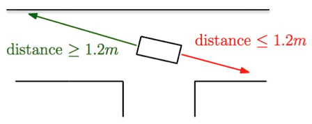
PICO is supposed to go right at the T-junction, but he goes left: that's because he detects the exit while he's slightly turned to the right with respect to the middle line, and detects a wall on his right, that means no free path in that direction. He achieves probably the fastest time, but it's too late and due to some luck at the second junction!
Software architecture
A first rough structure of our software could be represented in the following image:
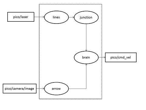
We decided to change it and reduce the number of nodes, since not all of them are strictly necessary. We defined our custom messages as well.
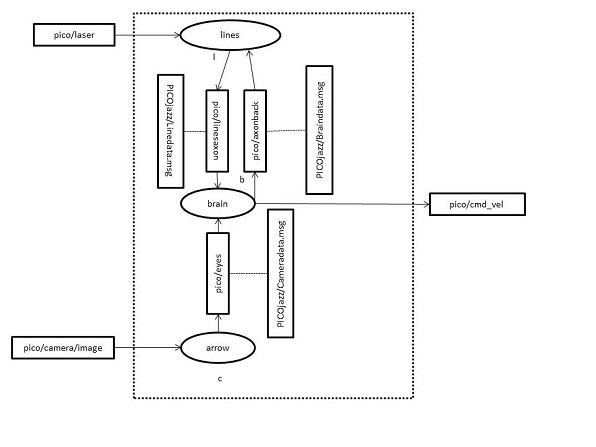
Nodes seem to communicate very well, and the messages are exchanged correctly.
Line detection node
We are going to robustly implement two functions in this node:
- One to know accurately PICO's position with respect to both right and left walls, therefore we'll be able to stand in the middle of the corridor for most of the time;
- One to find out which is the first horizontal front wall, and to compute the distance from PICO to this one.
To do so, we are going to loop infinitely over many functions described in the section "functions" below.
Functions
The core functions of the lines node are:
- laserCallback(): this function saves all the laser scanned points and plot them in an image, and saves the front, left and right distances to the wall;
- laserToPoints(): this function applies the Hough Transform to figure out the beginning and end points of each line detected. The next step is to sort the lines according to their position and orientation into 4 categories. Finally, we compute the distance to the closest wall;
- checkFreePaths(): this function checks, if we are closed to the first horizontal front wall, if there is any free path to the left, right or in front of PICO;
- sendToBrain(): this function is used to send only the relevant datas to the brain node.
Code illustration
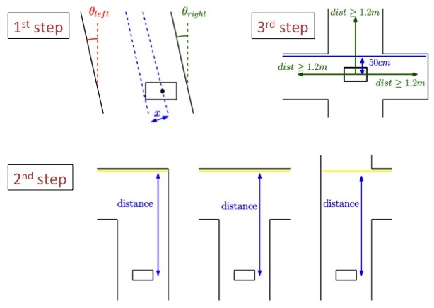
Here are represented the three main steps achieved in the Line Node:
- 1 - the orientation of PICO (theta) is computed from the two closest side walls, and then averaged. It's distance to the middle corridor line is also computed;
- 2 - the distance to the 1st front wall is computed, this will be the condition to stop PICO and check the free paths (see Step 3)
- 3 - as soon as PICO is in the middle of a junction, we use its left, front and right laser data to see if there is any free path. The condition is that the laser scan is above a certain threshold. This parameter was usually set between 1 and 1.2m according to the corridor width.
In the picture to the left are some examples to illustrate these steps.
Polar conversion
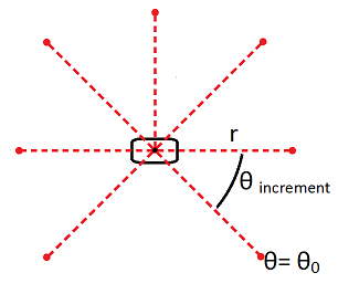
The output from the laser range finder are discrete points in space. These points represent a distant to an object (r) at a certain angle (θ) with respect to PICO. Once the angle of the first point and the angle increment of the sensor is known, each measured point can be represented in polar coordinates (θ,r). In the figure below, a representation of this is given.
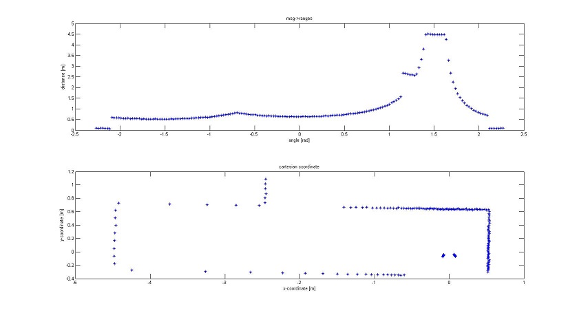
However, when we want to analyse PICO’s position with respect to surrounding object, the polar representation is not really efficient. This can be made clear with the following figure [EMC2012 group7]. The top picture of this figure is a representation of the laser points in the polar coordinates. From viewing this top graph, it is not immediately clear where the walls are with respect to PICO’s position (θ,0). The bottom picture represents the same points, but translated to Cartesian coordinates. It becomes immediately clear where the walls are. Now PICO is at the origin (0,0). The few points close to r=0 in the top picture and (0,0) in the bottom picture are the laser points which are reflected by PICO’s own body.
The first step has been made to identify the walls. However, the wall still only exist as a series of points. For the robot it is not clear when a wall begins or ends. It is also not clear if the walls are “vertical” or “horizontal” with respect to PICO. Vertical wall are parallel to PICO’s driving direction while horizontal walls are perpendicular to this direction. This distinction is necessary because horizontal walls may cause head on collisions while vertical walls may in their turn be useful to drive straight. It is decided to make an algorithm which provide us with a line representation of the walls. This representation can exists of a start point and endpoint of the line in Cartesian coordinates, or the orientation of the line can be given in polar coordinates. Where the distance R represents the shortest distance of the wall to PICO and the angle φ represents the lines orientation with respect to PICO (figure).
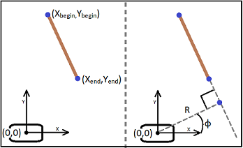
Both representations have their advantages and disadvantages. In the case of the begin and end point representation, the length of the line is known. However, to decide where and how the line is orientated with respect to PICO, a few more calculations need to be made. Goniometry is necessary to determine this orientation. The representation with the distance and angle give us the exact opposite information. The orientation and position of the line is known, but the length is unknown. This length cannot be reconstructed with only the information of the distance and angle. For a full and easy representation, it would be useful to have a combination of both cases; a begin and endpoint as well as the distance and angle.
First tactic, point-to-point evaluation
This tactic is based on evaluating each point with respect to its neighboring points. So instead of evaluating the whole collection of point, subsets of this collection are evaluated subsequently. These subsets consist of only a few points, for example 5. At the start of the algorithm, the first 5 points are chosen. To check whether these 5 points are in line, the formula for the Hough transform [[1]] is used:
[math]\displaystyle{ r = x * cos(\theta) + y * sin(\theta) }[/math]
In this formula, the x and y are the coordinates of the points. When the θ is varied from 0 to 2[math]\displaystyle{ \pi }[/math], a set of distances (r) is obtained. If the five points are on one line, this r will be the same for one choice of θ. This can be determined by checking at which θ the deviation between the distances is the smallest and whether this deviation is smaller than a certain value, e.g. if the deviation [math]\displaystyle{ (\sigma) }[/math] is smaller than 5% of the average [math]\displaystyle{ (\mu) }[/math] of the distance at this θ:
[math]\displaystyle{ \sigma(r_n) \lt 0.05 * \mu(r_n) }[/math]
If this is the case, the five points are on the line. The line now has an orientation of (r,θ) and also the start and end coordinates are known, these are coordinates of the first and last elements of the subset (point 1 and 5). If a line is found, a next point can be evaluated. It is checked whether this point is on the previously found line or not. If it is on the line, it will have the same orientation (r,θ). This can be checked by filling in the previously discussed Hough formula with x and y the coordinates of the point and θ the same as the θ of the line. If the distance is the same as the r found for the line, it is clear that the point is also on the line. The only thing that needs to be updated, is the endpoint of the line. This ‘extrapolation’ process keeps going on until a point is not on the line anymore. Then the next subset is evaluated. The same procedure is used to determine if a line exist in this set.
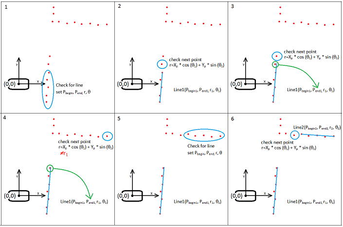
Second tactic, Hough transform
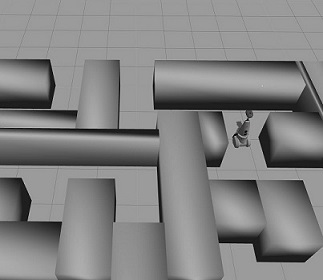
Because the poin-to-point evaluation might be prone to errors, it is decided to take another tactic. Our tutor pointed to us that within OpenCV there exist a function which searches for lines in pictures. This function would be useful to detect the arrow with the camera, but could also be used to detect the lines from the sensor data. However, the function uses an image as input, while the points are represented by values for x and y. To solve this problem, either the Hough transform function can be adapted, or the data points need to be converted into an image. It is decided to do the later because the Hough function already works. Adapting it to our problem could lead to troubles. To transform the data points into an image, we use the cv::imwrite function in OpenCV which transforms a matrix into an image. Each entry in this matrix will correspond to a pixel in the image. All the entries have a grayscale value from 0 to 255 or a colour representation of [r,b,g] where r,b and g also can have a value from 0 to 255. For our purpose it is sufficient to work with the grayscale values.
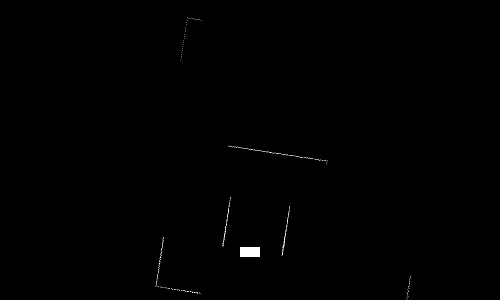
First it is necessary to define a matrix of size (r,c). The r and c represent the number of rows and columns respectively and are determined by the range of ‘sight’ of PICO’s laser. For instance, if we want to look 5 meter in each direction with centimetre accuracy, the matrix will be of size (1.000,1.000) . All values in this matrix are set to 0, or black in the image. Next, all the laser data points are evaluated. The x and y value of every point corresponds to an entry in the matrix. At this entry, the value is set to 255, or white in the image. An example of this can be seen in the next figures. The first picture shows a simulation of PICO in a maze. The next black and white picture shows the data points from PICO’s laser, transformed into an image.
It can be seen that the image is not a square. This is because the matrix which is constructed is also not a square. It was decided that the range of sight on the back of the robot does not need to be equal to the front range. PICO can detect object in front of him from a further distance than objects at his back. The white rectangle in the bottom centre is a representation of PICO itself.
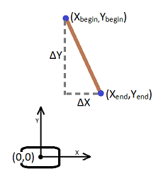
From this image the lines may be detected using the Hough transform function. The problem with this function is its robustness. The function might detect multiple lines on one wall. In order to cope with this problem, the lines are divided into four different types; left or right vertical walls and front or back horizontal walls. At first, a distinction needs to be made between horizontal and vertical walls. This is done using the difference between the points of the line. If ΔX is bigger than ΔY, the line is considered to be of the horizontal type. If it is the other way around, the line is of the vertical type.
The next thing to investigate, is the side on which the lines exist; left/right or front/back. To show how this is done, the left/right vertical walls are discussed. The distinction between front and back in the horizontal case is done in the same fashion.
The first idea of checking whether the walls were of type right vertical or left vertical, is described in the picture below. An average X is calculated using Xbegin and Xend; Xavg=(Xbegin+Xend)/2. This X corresponds to a point in the middle of each line. By evaluating whether or not this Xavg is bigger of smaller than the X of PICO’s position, the type of the wall would be known. This works well if PICO is nearly perfectly aligned. The picture below shows what happens when PICO is askew in a long wall.
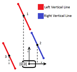
As can be seen from the picture, this algorithm is very robust. Line 1 is supposed be a line of type Right Vertical but is now recognized as a left line. This is because the average X is smaller than PICO’s position. This error can occur when the wall are far away and the robot is not aligned with the walls. To cope with this, the vertical lines have to be evaluated with respect to the middle of the corridor. A visualization of this is given in the figure to the right.
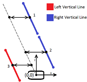
To do this evaluation (looking at figure on the left), the points on the middle of the corridor (grey dotted line) need to be found. It is decided to take points at the same height as the points of the lines, i.e. the Y values are the same. The difficult part is to get the X value of the points on the dotted line. For this, the orientation of the lines with respect to PICO needs to be known. In other words, one angle of the lines need to be known. It does not matter which angle is calculated, as long as the angle is used properly. Because ΔX can become very small, or even zero, if PICO is aligned to the wall, it is decided not to use the quotient between ΔX and ΔY to calculate the angle. This quotient could become zero or infinite. Therefor it is decided to take the length of the line piece instead. This will be made clear in the next figure. In this figure, only one wall is given to explain the method.
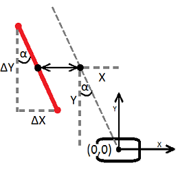
Now, the length of the line piece is calculated as:
[math]\displaystyle{ L=sqrt(\Delta X_2 + \Delta Y_2) }[/math]
Angle [math]\displaystyle{ \alpha }[/math] is than given by:
[math]\displaystyle{ \alpha = acos(\Delta Y/L) }[/math]
Point X on the middle of the line can then be calculated as:
[math]\displaystyle{ X = tan(\alpha)*Y }[/math]
Where Y is corresponds to some Y on the evaluated line. Now, every X on the line piece should be smaller or bigger than its corresponding X on the dashed line to be a left or right wall respectively. It suffices to only evaluate one X on the line piece, for instance Xbegin or Xend. This algorithm is more robust. The next figure shows the distinction between left or right vertical walls and front of back horizontal walls. The difference between horizontal and vertical is shown with the thickness of the lines. The distinction between left or right and front or back is made clear with either a white or grey colour.
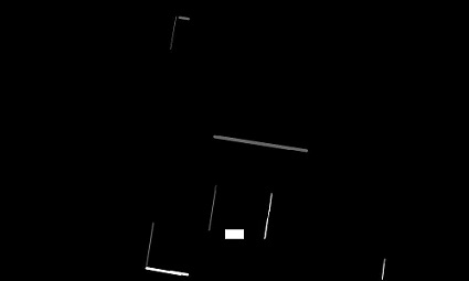
Now that the line are separated into four different types, they can be used to navigate PICO through the maze. For instance, if no horizontal walls are detected, PICO needs to just drive straight ahead. As soon as a front horizontal wall is detected, this means that a junction is ahead. The distance to this junction can be estimated and PICO can drive up to the middle of this junction. Using the vertical walls and the previously calculated α, PICO could align himself to the walls. Furthermore, the difference in distance between the left and right wall gives PICO a measure whether he is on the centre line or not.
Brain node
This node merges the information sent by camera topic and from the line detection node so to turn in the right way. In order to stay in the center of the corridor the brain tries to keep the difference betweeen the right and left radius from the line detected as low as possible.
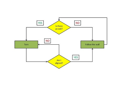
In a first time we opted for this flow-chart scheme, but when we started to implement it we realize that was too untidy for our purposes and we changed to an easier pseudo-code, focused in exploiting as much as possible our line detection algorithm. In this original algorithm the priority was to read the camera information; if there's none, turn right if possible. In case of dead end, turn 180° and keep following the right wall.
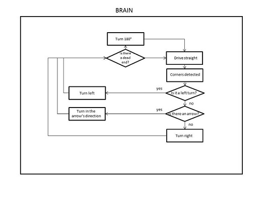
In the new approach, PICO always follows the right wall, until he detects an opening in the corridor. This is possible by reading the boolean data sent from the line detection node: one to stop and three for the junctions.
- cross=true when PICO reaches the center of a cross junction, thanks to the line detection data we can manage to stop in the center of the corridor, and then decide where to go.
- left,up,right=true when PICO recognizes an opening in the specified direction.
After elaborating all these data PICO can decide where to turn, always in agreement with the right wall following. Only in the T-junction case PICO has to check the directives coming from the camera topic.
Filling a matrix with the possible cases PICO can easy understand where is possible to go:
| Left | Up | Right | Decision |
|---|---|---|---|
| 1 | 0 | 0 | Left |
| 1 | 1 | 0 | Up |
| 1 | 1 | 1 | Right |
| 0 | 0 | 1 | Right |
| 0 | 1 | 1 | Right |
| 0 | 0 | 0 | Down (180°) |
| 0 | 1 | 0 | No junction |
The new brain node structure can be resumed with the following flow chart:
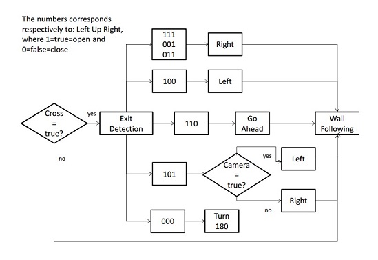
In the following picture there is the corrected brain flow chart, corresponding to the changes made immediately after the maze competition, now the 010 junction is included in cross=true (red block), and not in cross=false like in the previous one, in this way Pico after this particular case of cross can reset the front distance value and continue solving successfully the maze.

The lines node also send one more boolean variable for the safety condition:
- drive=true, meaning that PICO can drive because is in a safety zone.
Also the scan ranges needed for the wall following and the dead end zone are sent from the lines node, these are an avarage of the north, right and left scan.
Functions
The core functions of the brain are:
- move (): simplifies sending velocity commands to the base. It has 4 parameters: linear speed, linear speed's sign, angular speed, angular speed's sign. It's used in other functions.
- turnPI (), turnRIGHT (), turnLEFT () : turn on the spot for PICO, with a fixed degree range. The turning function is the same of the corridor competition: a time counter with a loop that allows to achieve the desired angle with the selected velocity, thus 90° for normal turning and 180° when PICO is in a dead-end point.
- exitDetection (): according to messages received by the brain from the lines node,PICO detects the junctions.
- WallFollowing() : The wall following function has been recycled from the corridor competition in a first moment, and was improved. A further explanation is given below, since this is one of the most important modules of the robot.
Line follower
Since we don't have a robust way to handle the safety condition, we need to avoid at all costs the walls.
We first divide the corridor into a safe zone and a dangerous zone. Everything further than 1,5 cm from the middle corridor line is considered as dangerous, thus requires a correction in PICO's orientation. The simple controller takes into account the distance from the middle corridor line dx (cm), whose sign depends on which side of the corridor PICO is and the angle with respect to the walls (degrees), whose sign depends on the left or right orientation. The controller sums up angle and distance with their absolute value, before dividing it by an arbitrary constant K:
[math]\displaystyle{ \dfrac{\left |(\theta+dx)\right |}{K} }[/math]
The correction is sent as a parameter to the move() function.
If PICO is outside the safe "belt", generally four cases can occurr:
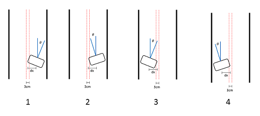
- 1) PICO is on the right side of the corridor, with positive angle with respect to the mid line
Correct orientation driving to the left.
- 2) PICO is on the right side of the corridor, with negative angle with respect to the mid line
Go straight, he's already in the correct direction.
- 3) PICO is on the left side of the corridor, with positive angle with respect to the mid line
Go straight, he's already in the correct direction.
- 4) PICO is on the left side of the corridor, with negative angle with respect to the mid line.
Correct orientation driving to the right.
Arrows detection Node
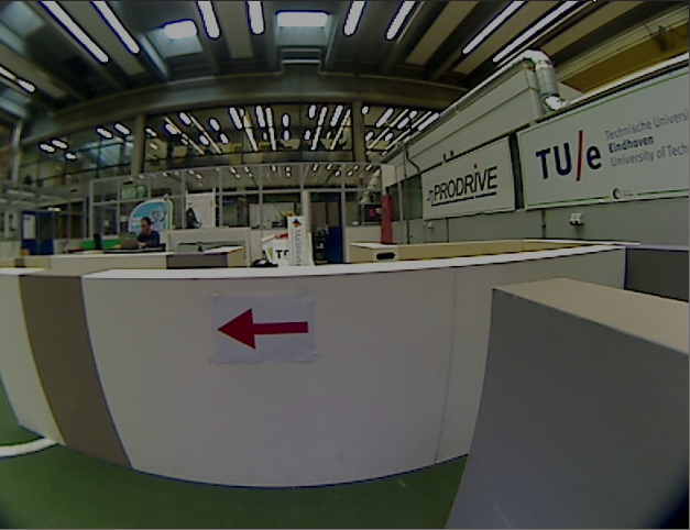
The strategy for the arrow recognition is to create a template of an arrow and check the obtained camera image for this template. This is implemented by making the following steps:
- Obtain camera image from PICO
This camera image is not being calibrated or modified otherwise. This is not required since we will use a template based algorithm to detect the arrow.
- Transform this image to a HSV (Hue, Saturation, Value) image
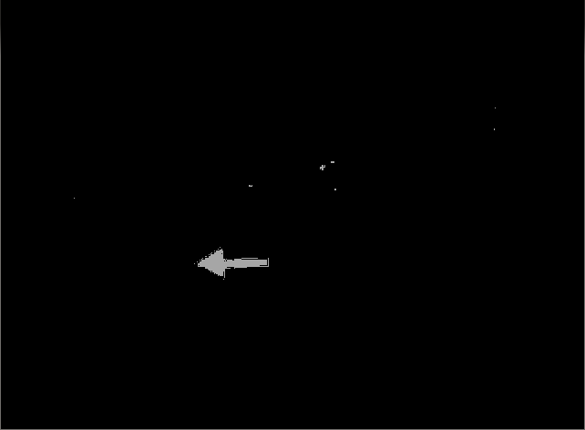
- Tresholding this image to obtain a wide enough range of the red colors of interest
This thresholding is done by obtaining the HSV value from the arrow is found by using a color picker tool within a image editor program. A wide range of HSV values is used to make a robust arrow recognition, noise in the image will not be a problem. The tresholded image will contain all the red objects in the camera image. The range of HSV values is the minimum (150, 100, 80) till the maximum (240,255,255).
- Since a binary image is obtained after tresholding a template matching algorithm can be used
- A template image is created which contains an arrow, this image is made in a simple image editor only once
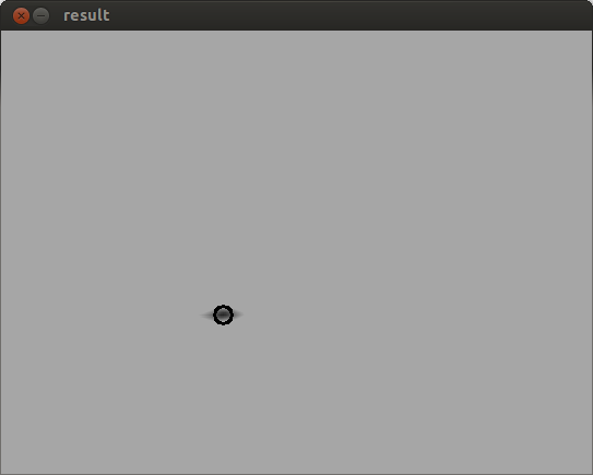
- The openCV function matchTemplate is used to compare the template image with the image from the camera of PICO. This function in combination with the CV_TM_SQDIFF_NORMED matchTemplate method gives a normalized score from 0 - 1 which represents the similarity inverse, 0 being an exact match.. An image representing this score can be seen below, the circle represents the found arrow.
- A threshold is set to 0.5, until this value an arrow will be accepted.
- By using only a left image template it is prevented that an arrow to the right will be detected, neither other red object within the environment will be recognized
- Since the arrow in the corridor will be horizontal placed the algorithm does not cope for a rotated arrow
Since we are using a right-wall following algorithm, only an arrow to the left is interesting for us. A template of the left arrow is used for the comparison algorithms. This is tested with several of earlier created BAG files to verify its robustness of actually only detecting arrows to the left. No arrows to the right are detected and no red objects in the environment are recognized as being an arrow.
The algorithm is tested during the final test before the contest. The algorithm is not used during the final competition since the camera node in real-time was too slow to give feedback to PICO. The algorithm itself did work properly and the arrow was recognized for an interval of +- 50 centimetres.
Things that could be implemented to make the algorithm better and faster are:
- Cropping the camera image to a smaller image in which an arrow could be, this will make the code faster
- Scaling the template image to be able to detect an arrow from greater distance
- Information from an arrow could also be used when PICO is not in a T-junction, to avoid PICO to enter dead ends in the maze for example. The arrow to the left at the final competition maze could have been used to override a possible decision of the brain to enter one of the dead ends in the beginning of the maze.
- Also detect arrows pointing to the right. This must be done for the previous point and if a maze solving algorithm is used (No right wall following)
Functions
Work division
We decided to divide the work to optimize the available time:
- Erik -> Image acquisition, Camera and everything concerned with the arrow detection
- Jordi -> Line detection algorithm and junction recognition
- Martin -> Line detection algorithm and junction recognition
- Marcello -> Software architecture, inputs/outputs, custom messages, nodes
- Luigi -> Working on previous algorithm, brain node and take-exit functions using the right wall following method
Tests
First test (19/9)
Experiments are performed on PICO, however the testing did not go as planned. PICO had to be resetted sometimes and did not respond to our commands as expected. The data shown in the terminal however, did show the proper values while running.
Second test (20/19)
We experienced again some connection issues. We were able to move the robot, and again some delay seemed to occur. The discharged batteries have put a premature end to our tests.
Third test (24/9)
We had 15 minutes to verify our new code, developed in a few hours of this very day, that allows PICO to turn on the spot. Everything worked fine, but improvements have to be made to get a more robust algorithm and, most of all, a fastest one: the turning maneuver is too slow.
Fourth test (11/10)
In this test we used the ROS record function in order to check in different situations what PICO can elaborate from his sensors and from the camera thanks to our line detection and arrow detection algorithm. We recorded in various .bag files the only three topics in which we were interested: camera,laser and odom. Now we can work in this week-end to improve our codes with the real data.
Fifth test (17/10)
Today, we tried to deal with all the different types of junction. It was successful except in the deadend. To turn, we are using a counter, so it is a time-based turn. As the robot field is not perfectly flat, we lack of precision at the end of the U-turn. We are going to work on a solution using the orientation of PICO w.r.t. the right/left wall at the end of the turn to have a higher accuracy. Then, it will be a 2-steps turn:
- 1st step: turn nearly till +/-90 or +180 degrees using a counter;
- 2nd step: end the turn using the orientation of PICO according to the walls.
Sixth test (21/10)
This was our last chance to test the whole software and especially the new camera node. We experienced some problems with the 180° degrees turning due to specific wall configurations. Unfortunately, the camera node didn't work as expected. We tried to change the resolution of the image used as template, but we needed more time to continue the tests. We decided thus not to include it, since it's unreliable. We did tune the wall following algorithm though, and other parameters useful for the exit detection function.
Possible (and impossible) problems
Simulation/Reality discrepancies
During our real tests, the simulations and -unfortunately- the final competition, we realized that something can always go wrong. Even though we try to achieve a robust code, the robot can behave in an unexpected way. Some noticeable examples are related to PICO's movements: they don't correspond exactly to our commands, probably because of friction of the wheels and the non-idealities of the environment, i.e. non straight walls. We computed how to turn accurately of 90° and 180° using the velocity commands, anyway we obtain often an error of about plus or minus 2 degrees. We are not able to control this error with our functions so we decided to compensate for it only after the turning function has been completed, using the wall-following feature. Sensor issues are also a thing to be aware of: pre-processing the data is always a must, because sensor and environment noise is an omnipresent fellow during our maze exploration and doesn't show up in the simulations.
Coding issues
Our programming skill is very basic, since none of us has a computer science background. The code shape could get better and sometimes it's hard to implement an idea from the pseudo code to the actual code; because of the lack of experience and solutions, our code often boils down to a series of "if" conditions and evaluations.
- For instance, we've not been able to handle the tricky safety condition. We don't want PICO to crash against the wall, so for emergency cases we need it to stop. We have not managed yet to restart him to continue his path. Unfortunately when PICO is so close to the walls, (that normally shouldn't happen if our wall-following function works correctly), PICO suddenly stops and finishes his run! An efficient way to solve this issue must be found.
- Some readings seem to have no sense. In the first three loops, scan_ranges gives back only null values. Actually we don't know why and we decided to exclude these values from some functions, like the turning 180° for the dead end because they were inhibiting its operations.
- Always regarding the scan ranges we don't use the first and last 10 scans of every loop because the first 7 laser scan hit PICO's body and overcome our working, we decided to discard other few values to maintain a certain security extent.
Timing issues
Nodes have to communicate one to another. Even if we think this is not the case, since we have only three nodes working together and exchanging informations, delay and/or data overlapping can occur, if buffers are not set appropriately or loop spin rates are wrongly chosen.
Hardware issues (Virtual Machines)
Last, but not least, are the problems related to hardware requirements for the simulation on Gazebo. We tried to simulate PICO in the maze with two virtual machines, and PICO would not turn correctly on the spot. Probably that happens because of the insufficient computational power, since the hosting machine is running on the background, memory and CPU are limited and the performance is poor, not as a plain Ubuntu dual boot installation.
Could it have gone better?
Yes, it could. Apart from the error in the final competition, there's large room for improvement.
- We did not have a reset condition after the safety condition was triggered.
- We could have come up with a line detection algorithm since the corridor competition, to avoid the waste of time due to an almost complete re-design of the algorithm.
- A better laser data filter should have been designed, since we just use a resolution filter (though it has proven to be adequate).
- We weren't able to finish the camera node in time to have at least 2 hours to test it.
- We did not implement any maze solving algorithm, due to the lack of time.
- In the beginning we were not familiar with Ubuntu, Qtcreator and the SVN repository, all of this resulting in a loss of time.
- Work division had to be rethinked.
Other improvements?
- We didn't write an elegant code.
- We didn't use the odometry information.
- Path planning, localization, learning elements?
