Embedded Motion Control 2013 Group 10: Difference between revisions
| (143 intermediate revisions by 3 users not shown) | |||
| Line 1: | Line 1: | ||
= Group Name = | |||
Team Picobello | Team Picobello | ||
= Group Members = | |||
<table> | <table> | ||
<tr> | <tr> | ||
<td width="150px"><b>Name:</b></td> | <td width="150px"><b>Name:</b></td> | ||
<td width="120px"><b>Student id:</b></td> | <td width="120px"><b>Student id:</b></td> | ||
<td width=" | <td width="400px"><b>Email:</b></td> | ||
</tr> | </tr> | ||
<tr> | <tr> | ||
<td>Pepijn Smits</td> | <td>Pepijn Smits</td> | ||
<td>0651350</td> | <td>0651350</td> | ||
<td>[ | <td>p [dot] smits [dot] 1 [at] student [dot] tue [dot] nl</td> | ||
</tr> | </tr> | ||
<tr> | <tr> | ||
<td>Sanne Janssen</td> | <td>Sanne Janssen</td> | ||
<td>0657513</td> | <td>0657513</td> | ||
<td>[ | <td>s [dot] e [dot] m [dot] janssen [at] student [dot] tue [dot] nl</td> | ||
</tr> | </tr> | ||
<tr> | <tr> | ||
<td>Rokus Ottervanger</td> | <td>Rokus Ottervanger</td> | ||
<td>0650019</td> | <td>0650019</td> | ||
<td>[ | <td>r [dot] a [dot] ottervanger [at] student [dot] tue [dot] nl</td> | ||
</tr> | </tr> | ||
<tr> | <tr> | ||
| Line 29: | Line 29: | ||
<td>0649843</td> | <td>0649843</td> | ||
<td>[ | <td>t [dot] korssen [at] student [dot] tue [dot] nl</td> | ||
</tr> | </tr> | ||
</table> | </table> | ||
== | =Introduction= | ||
To | |||
[[File:jazz.jpg|left|bottom|200px]] | |||
Nowadays, many human tasks have been taken over by robots. Robot motion control and embedded motion control in the future allow us to use robots for many purposes, such as health care. The (humanoid) robots therefore have to be modeled such that they can adapt to any sudden situation. | |||
The goal of this project is to get the real-time concepts in embedded software design operational. This wiki page reviews the design choices that have been made for programming Jazz robot Pico. Pico is programmed to navigate fully autonomously through a maze, without any user intervention. | |||
The wiki contains three different programs. The first program was used for the corridor competition. In this program the basic skills like avoiding collision with the walls, finding corners and turning are implemented. | |||
After the corridor competition, a new design strategy was adopted. The second program consists of a low level code, namely a wall follower. By keeping the right wall at a fixed distance from Pico, a fairly simple, but robust code will guide Pico through the maze. | |||
Besides this wall follower strategy, a high level approach was used. This maze solving program uses wall (line) detection to build a navigation map, which Pico uses to create and follow path lines to solve the maze. To update the position of Pico, the odometry information, local and global maps are used. | |||
The latter two programs use Pico’s camera to detect arrows in the maze that point Pico in the right direction. | |||
=Data processing= | |||
Pico outputs a lot of sensordata. Most of the data needs to be preprocessed for use the maze-solving algorithm. The odometry data, laserscandata and imagedata are discussed below. | |||
==Odometry data== | |||
One of the incoming data types is the odometry. The odometry information is based on the angular positions of the robot wheels. These angular positions are converted into a position based on a Cartesian odometry system, which gives the position and orientation of Pico, relative to its starting point. For the navigation software of Pico, only the x,y-position and <math>\theta</math>-orientation are of interest. | |||
Due to slip of the wheels, the odometry information is never fully accurate. Therefore the odometry is only used as initial guess in the navigating map-based software. For accurate localization, it always needs to be corrected. | |||
This correction is based on the deviation vector obtained from the map updater. This deviation vector gives the (x,y,θ)-shift that is used to fit the local map onto the global map and therefore represent the error in the odometry. Because of the necessary amount of communication between the parts of the software that create the global map and the part that keeps track of the accurate position, these parts are programmed together in one node. This node essentially runs a custom SLAM (Simultaneous Localization and Mapping) algorithm. | |||
==Laserscan data== | |||
To reduce measurement noise and faulty measurements the laser data is filtered. Noise is reduced by implementing a Gaussian filter, which smoothens each data point over eight other data points. | |||
<math>G(x)=\frac{1}{\sqrt{\sigma \pi}}e^{\frac{-x^2}{2 \sigma^2}}</math> with <math> \sigma = 2.0 </math> | |||
Faulty measurements are eliminated in three different ways. First data points which deviate a lot from their neighbors are ignored in the Gaussian filter so that the filter does not close openings. When ignoring data points the Gaussian is normalized based on the used points. | |||
Secondly the first and last 15 data points are ignored, decreasing the angle of view by 7.5 degrees at each side, but preventing the robot to measure itself. At last, only data points are used which are between a certain range, not only to prevent measuring the robot itself, but also to eliminate outliers. | |||
==Arrow detection== | |||
===Binary image=== | |||
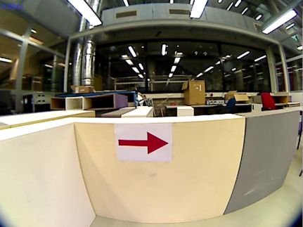
From a full color camera image we want to determine whether there is an arrow and to determine its direction. Because this full color camera image is too complex to process, we transform it into a binary image. Since the arrows used in the competition are red, everything that is red (with a certain margin) is made white and the remaining is set as black. | |||
===Canny edge detection=== | |||
Next edges are detected with a canny edge detection algorithm from openCV. This algorithm uses a Gaussian filter to reduce noise, similar to the one explained above. But it also uses the gradient of this Gaussian filter. At and edge there is a very strong transition from white to black, resulting in an extreme value in the gradient. So by thresholding the gradient, edges can be detected. | |||
===Find contours=== | |||
The binary image from the canny edge detection is used as input in the FindContours function from openCV. This function finds contours by connecting nearby points, giving a vector of contours as output. Each contour consists of a vectors filled with points. | |||
===Arrow detection=== | |||
[[File:arrow1.png|thumbnail|right|200px|alt=|figure 1 Arrow direction]] | |||
[[File:arrow2.png|thumb|200px|alt=|figure 2 Arrow shape]] | |||
Finally the image is processed so that we can start detecting arrows. Arrows are detected in two steps. First the ratio of the height and the width of each contour is determined, to see if the contour can be an arrow, see figure 1. The arrow used in the competition has a ratio of 2.9, with a lower and upper bound, this results in: | |||
<math> 2.4 < \frac{dx}{dy} < 3.4 </math> | |||
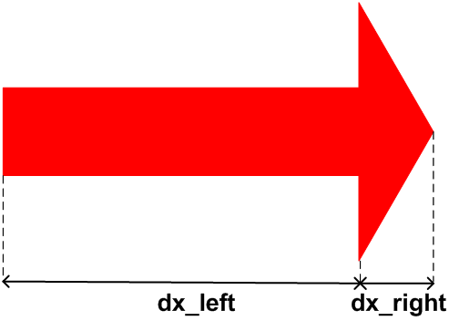
Next if a contour can be an arrow, the direction is investigated. This is done by determining the ratio of dx_right and dx_left, see figure 2. If the largest width (dy) is shifted towards the right dx_left > dx_right and the other way around. With some lower and upper bound this results into: | |||
Right arrow if: | |||
:::<math> dx_{left} > \frac{5}{4} dx_{right} </math> | |||
Left arrow if: | |||
:::<math> dx_{left} < \frac{4}{5} dx_{right} </math> | |||
No arrow if: | |||
:::<math> \frac{4}{5} dx_{right} <= dx_{left} <= \frac{5}{4} dx_{right} </math> | |||
If the largest width is in between the margins, the contour cannot be an arrow and is treated as such. This may not be the most robust way to detect an arrow, but during the tests it seemed to work just fine. A few other methods that can be used or combined to make the arrow detection more robust are circularity, shape matching, matching of moments or finding lines with the Hough transform. | |||
{| class="wikitable" | |||
| [[File:camera image538.png|thumb|alt=|figure 3 Camera image]] | |||
| [[File:binary image538.png|thumb|alt=|figure 4 Binary image]] | |||
| [[File:canny edge detection538.png|thumb|alt=|figure 5 Canny edge detection]] | |||
| [[File:find contours538.png|thumb|alt=|figure 6 Contours]] | |||
| [[File:arrow detection538.png|thumb|alt=|figure 7 Arrow detection]] | |||
| | |||
|} | |||
=Program 1: Corridor Challenge solver= | |||
==Wall avoidance== | |||
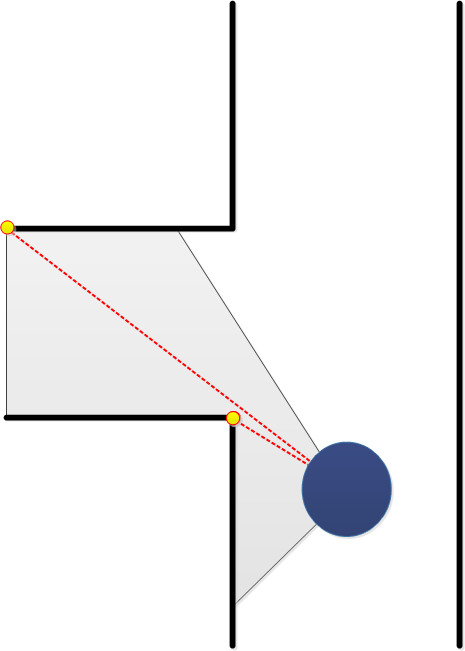
[[File:Wall_avoidance.png|thumb|100px|alt = |figure 8 Wall avoidance]] | |||
The function ‘wall_avoidance’ has the simple function of preventing collisions. It therefore overrules the determined velocity and rotation if an object is very close. | |||
The function calculates a region in which no objects are allowed. This region is elliptically shaped and its parameters are velocity and rotation rate dependent. This makes it possible to drive near objects if the velocity is low, for example when driving in a narrow corridor. | |||
This function could be improved by not only using the rotation rate but also the rotation direction. Now Pico may stop when driving to the right if an object is to the left. The ellipse should then consist of more than two parameters. | |||
. | |||
==Edge detection== | |||
For the corridor competition, Pico should first be able to detect an outside corner (see figure 9). To detect corners, the laser range data is used. | |||
The robot searches left and right for large differences in wall distance. If the length ratio between two neighboring ranges exceeds a certain threshold, the position (1) of the outside corner is saved. Also the side of the corridor is set to left or right. If the first corner has been found, Pico searches at this side for other corners. This search algorithm starts at the first corner and checks for the shortest laser range distance. This coordinate is saved as second edge position (see figure 10). The coordinates of the edges are sent to the make turn function, which controls Pico’s movement. | |||
If Pico is past the first corner, the first algorithm explained above cannot recognize this first corner anymore. To avoid problems, the second algorithm is activated for both the first and last corner (see figure 11). | |||
{| class="wikitable" | |||
|[[File:edgescan1.png|thumb|180px|alt=|figure 9 Detect first edge]] | |||
|[[File:edgescan2.png|thumb|180px|alt=|figure 10 Detect second edge]] | |||
|[[File:edgescan3.png|thumb|180px|alt=|figure 11 Detect both edges when pico has turned]] | |||
|} | |||
==Turning into the corridor== | |||
[[File:corner detection.png|thumbnail|150px|right|alt = |figure 12 Make the turn]] | |||
If the first corner is passed, a boolean is set to true and the centering algorithm is replaced by the algorithm used to make a turn. This algorithm uses the two corners of the side exit determined by the corner detection algorithm. | |||
First it drives a little towards the side exit but prevents a collision with the first corner. If the middle of the side exit is reached, L1 = L2 in figure 12, Pico is turned until both angles to the corners are equal, Theta1 = Theta2. It then drives in the exit while keeping the difference between the distances to the corners within a margin. If the absolute values of the angles to the corners are both larger than 90 degrees, the make turn algorithm is switched off and the centering algorithm is switched on again. | |||
The algorithm could be improved by not only using the distances to the corners but also preventing coming to close to the other wall of the corridor. This is not a big problem since the wall avoidance algorithm prevents collisions. | |||
. | |||
==Centering algorithm== | |||
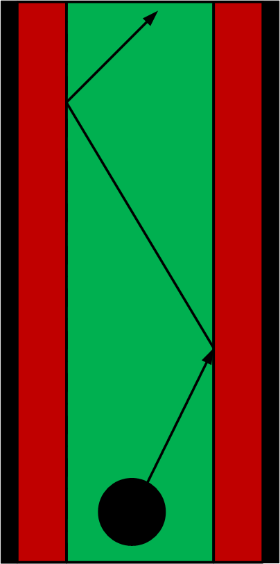
[[File:Center Corridor.png|thumb|100px|alt =|figure 13 Centering algorithm]] | |||
This algorithm uses the shortest length to left and right and the corresponding angle. These properties are derived in the function ‘detectWalls’ and put together in one variable. Its output is a forward velocity and a rotation rate. | |||
First the current corridor width is determined by summing up the shortest distances to the left and the right. This sum is wrong when a side exit is reached, but this is not a problem since a different function is used to make the turn. | |||
If the distance to one of the sides is smaller than one third of the corridor width, it is determined if Pico is facing the wall or the middle of the corridor, see the red area in figure 13. If it is facing the wall it is turned back without driving forward, if it is facing the middle, it drives with a velocity of 0.2. | |||
If Pico is in the middle third if the corridor, it also drives forward with a velocity of 0.2, see green area in figure 13. | |||
The function could be improved by determining the angle that has to be made to face the right direction. This angle should not be used as the rotation rate, but the odometry should be used to determine if the preferred angle is reached. | |||
Another improvement would be a better controller, which also steers if Pico is still in the middle part of the corridor. This was not implemented since in this stadium the function wall_avoidence was still very basic and could not handle driving and steering well. | |||
. | |||
==Program structure== | |||
[[File:structure corridor.png|thumb|right|100px|alt =|figure 14 Structure of the corridor competition program]] | |||
This program has a single node structure. All functions are defined internally in a so called ‘awesome node’. The wall avoidance has the highest priority in the node to avoid wall collision. The second most important function is the centering algorithm. if the edge detection has detected a side corridor, the turning algorithm is activated. A schematic view is shown in figure 14. | |||
. | |||
==Program evaluation== | |||
During the corridor competition, the program was fixed, but some bugs came up. The functions stay in middle and wall avoidance worked well, but during the last simulations before the corridor competition, the corner detection showed some undesired results. | |||
The first and second corners are detected correctly. While turning however, Pico starts to recognize an outside corner at the end of the corridor, as depicted in figure 15. This third corner confuses the program, because the turning algorithm now questions which corners to use as a reference. Due to this unexpected corner, Pico was not able to solve the corridor competition. Therefore two new strategies were developed to win the upcoming competition: solving the maze. The wall follower and high-level maze solving program. | |||
[[File:edgescan4.png|thumb|200px|alt = |center|figure 15 Problems occur when Pico turns]] | |||
=Program 2: Wall Follower= | |||
==Structure== | |||
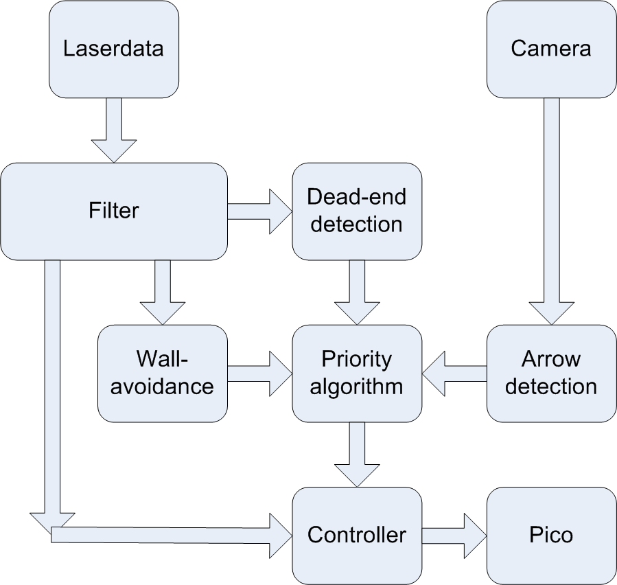
The wall follower is constructed as shown in figure 16. First the laserdata is used for wall-avoidance as explained above and dead-end detection. Also the cameradata is used to detect arrows. Based on these three modules, the priority algorithm decides which action to take and is more or less the ‘brain’ of the program. Depending on the desires of the priority algorithm, the controller makes sure Pico either follows the right wall or makes a left turn. | |||
[[File:Structure_wallfollower.png|thumbnail|center|300px|alt=|figure 16 Structure of the wall follower.]] | |||
==Dead end detection== | |||
[[File:Dead_end.png|thumbnail|right|300px|alt=|figure 17 Dead-end detection.]] | |||
The main reason for dead-end detection is to make sure Pico does not drive into corridors without an exit or crossing at the end. The main idea is that if dead-ends can be detected, Pico returns immediately, which can save a lot of time. | |||
Dead-ends are detected by closed contours in the filtered laser data. To find closed contours the distance (dL) between two subsequent data points is calculated with the cosine rule: | |||
<math> dL = \sqrt{R_1^2+R_2^2-2R_1R_2cos(d\theta)} </math> | |||
If two points are inside a closed contour, the distance between those points is small, see the red dots in figure 17. While they are not inside a closed contour the distance is large, see the green dots in the same figure. To determine whether the points are in- or outside a closed contour we use a threshold, <math> dL < dL_{max} </math>. | |||
Finally we say there is a dead-end, if the contour is closed for a certain range of points. Testing confirmed that a range of -60 to 60 degrees ensures that Pico does not only correctly detect dead-ends, but also detect them from a reasonable distance. | |||
If a dead-end is detected the robot turns left, until it finds an opening within the -60 to 60 degrees ranges and then continues following the right wall. | |||
==Priority algorithm== | |||
There is a simple decision making algorithm that can decide to follow the right wall, turn left or stop. This is done by checking the states of different modules and their desires. The wall follower always wants to follow the right wall, except when there is a dead-end or an arrow to the left. In these cases the robot will turn left. Arrows to the right are ignored, since the robot already wants to go that way. Finally if the robot is too close to a wall the wall avoidance wants Pico to stop. This results in the following priority: | |||
Wall avoidance > Arrow detection > Dead-end detection > Wall follower | |||
==Controller== | |||
[[File:Min_distances_total.png|thumbnail|upright|400px|alt=|figure 18 Left) Minimal distances within three different areas. Right) Proportional controller.]] | |||
The controller is a simple proportional controller, based upon a few essential values, defined in figure 18 | |||
The essential values are the closest distance to the wall and their corresponding angles, defined in three different areas. | |||
:Left: -130 until -10 degrees. | |||
:Front: -30 until 30 degrees. | |||
:Right: 30 until 130 degrees. | |||
The wall follower always wants to keep <math> L_{right} </math> at a distance (d) of the wall, see figure 18 | |||
The controller sends an angular velocity (<math> \dot{\theta}</math>) to Pico, | |||
which is proportional to the difference between this setpoint and the minimal distance to the right wall. So | |||
:<math>\dot{\theta}\sim L_{right}{-}d</math> | |||
To make sure that the robot drives as straight as possible, the angle towards the closest distance at the right wall (<math> \theta_{right} </math>) is kept at 90 degrees. Also | |||
:<math>\dot{\theta}\sim\theta_{right}{-}\pi/2 </math> | |||
The linear velocity (v) is also controlled proportionally. If <math>L_{front}</math> is large, the path is clear and meaning it is fairly safe to drive fast. So | |||
:<math>\mathbf{v}\sim L_{front}</math> | |||
Both linear and angular velocity are limited by 0.2 and 0.7 respectively. | |||
==Program evaluation== | |||
A wall-follower is a fairly simple, but very robust program. It also benefits from dead-end and arrow detection; two features which both highly increase the performance. On the other hand, the simplicity of the program will eventually prevent the program from becoming highly intelligent. The lack of a map makes position determination, decision making and complex maze configurations hard to deal with. This is the program we used during the final competition, which resulted in the first place. | |||
=Program 3: Map based strategy= | |||
==Program Structure and introduction== | |||
[[File:structure map based.png|thumb|200px|left|alt = |figure 19 Structure of map based strategy]] | |||
The wall following code is effective and robust, but a more challenging code was created. Here a total map of the maze is created and used to determine its path. | |||
The laser data is filtered with the aforementioned Gaussian filter. | |||
A local map is created from the laser data only. This results in lines representing the visible walls which are then sent to the map updater node. Then the local map and odometry are updated with an optimization algorithm to match the global map. The global map is updated and visualized together with the driven path. | |||
This map is then sent to the node ‘create path’. This function also receives an arrow direction if an arrow is detected. If a service is asked from the ‘Line follower’ the end point of the last path is reached and a new one has to be sent back. This path consists of a line with an end point and an absolute angle that has to be matched with the odometry at the end of the line. | |||
It is also possible to do this path planning with the local map, but then it is not possible to create a path going back when a dead-end is found. The global map consists of many optimization steps and is therefore much more reliable than the local map. | |||
The line follower receives the new path and a global position. The line follower drives to the end of the line if the shortest distance to the line stays within a margin. Otherwise it will first drive back to the line and then again to the end. | |||
Then the earlier described ‘wall avoidance’ node checks if no objects are close and sends the velocity and rotation rate to Pico. | |||
The main advantage of this map based navigation is that arrows can be used smartly and the path planning allows for feed forward where the wall follower only uses feedback. The path planning algorithm can be improved for creating smooth corners and determining the path before the end of the line is reached. In this way to the total maze can be driven with the maximum velocity of 0.2. | |||
==Local map creation== | |||
To create a useful and efficiently containable map, the laser data must be reduced to the essential information it contains. Since the walls scanned by the laser data are in good approximation straight, these can be represented by line segments. Before any search for lines is done, the laser data is filtered with the specialized Gaussian filter ([[#Laserscan data]]). | |||
Local map | |||
To obtain the line segments, the approach proposed by group 5 of 2012 ([[http://cstwiki.wtb.tue.nl/index.php?title=Embedded_Motion_Control_2012_Group_5#Node-based_Mapping]]) is adopted. The method is implemented as follows. | |||
create a line between point 1 and point 2 of the LRF data (LINE class) | |||
l = current line (defined by first two points) | |||
FOR all data points | |||
p = current point | |||
s = current new line segment (defined by end of current line and current point) | |||
nFaulty = current number of points found that do not belong to s | |||
IF ( nFaulty < n_max AND angle between l and s < angle_max AND length of s < length_max) | |||
// Point is good and can be added to the line | |||
replace end point of l by current point | |||
nFaulty := 0 | |||
ELSE IF ( nFaulty >= n_max ) | |||
add current line to array of lines (map) | |||
IF ( length of s > length_max ) | |||
// There is a jump in the laser data, so an outer corner point is found | |||
//initiate new current line with | |||
start point := saved first faulty point | |||
end point := current point | |||
ELSE | |||
// The angle was too large, so an inner corner point is found | |||
// initiate new current line with | |||
start point := end point of old current line | |||
end point := current point | |||
END | |||
ELSE | |||
IF (first faulty point found) | |||
save current point to start potential new line from | |||
END | |||
nFaulty ++ | |||
END | |||
END | |||
After this original setup, an extra if statement was added to keep the algorithm from adding line segments that are too long to a line (possible if there are two jumps in laser data right subsequent of each other. | |||
Implementing this routine and testing it showed that the resulting number of lines is too high. Especially the laser data near the robot is relatively noisy. This is most likely due to the fact that the absolute error in laser range data stays about equal, such that the relative error on small measurements is relatively large. Also the points near the robot are relatively close together (order of millimeters), so that the error in the laser data quickly results in a large angle between the current line and the to-be-added line segment. The algorithm recognizes this as being an inner corner, so it does not add the line segment to the current line. | |||
To deal with this, an extra filter is implemented over the lines, which combines lines if their difference in angle is within a certain range which is narrower than used in the original algorithm. Also short lines are combined with one of their direct neighbours. This way, short lines that occur due to noise are filtered out and corners are sharpened. | |||
The additional filters reduce the number of lines found from around 60 to less than 10. | |||
==Global map== | |||
For navigation purposes, a global map is desired. This global map can be built out of the local maps from each time step. However, these local maps are saved in a vector format with the robot fixed reference frame as a base. The global map needs to be defined in a global perspective. Hereto the local map is transformed to a global vector base. Additionally, the position of the robot in the map is required. This is however a nice byproduct of the process of creating a map. The noisy and error sensitive odometry information can be enhanced using the translation and rotation necessary to fit the local map to the global map. | |||
Firstly, the global vector base must be defined, this can be done using the robot’s initial position (at the start of the program). This position and orientation is chosen as the (x,y,theta) = (0,0,0) point of the global map. | |||
Next, the local map created by the robot needs to be translated and rotated to the global base. This can be done by using an estimation of the robot’s position given by the odometry information ([[#Odometry data]]). Every point in the local map can be transformed to a point in the global map using the following transformation: | |||
<math>\mathbf{x_{global}} = \begin{bmatrix} | |||
cos(\theta) & -sin(\theta) \\ | |||
sin(\theta) & cos(\theta) \\ | |||
\end{bmatrix}. \begin{bmatrix} | |||
x_{local} \\ | |||
y_{local} \\ | |||
\end{bmatrix}+\begin{bmatrix} | |||
x_{robot} \\ | |||
y_{robot} \\ | |||
\end{bmatrix}.</math> | |||
[[File:world_with_global_map.png|thumb|200px|alt =|figure 20 Simulation maze representation]] | |||
[[File:global_map.png|thumb|200px|alt =|figure 21 Pico's global map representation]] | |||
where \theta is the orientation of the robot in the global system, the local coordinates are the coordinates of a point with respect to the robot fixed frame and the robot coordinates depict the robot’s position in the global frame of reference. This creates a local map in the coordinate system of the global map. This map can now be added to the global map. Using this method it is already possible for a human to get some understanding of the layout of the maze. An example can be found in figures 20 and 21. | |||
To create a better map, it is possible to start by replacing lines in the global map by their corresponding lines in the local map. However, as can be seen in figures 20 and 21, the lines drift off as the robot drives through the maze. This can be attributed to the accumulating error in the odometry information. | |||
The error can be accounted for by fitting the new local map to the old global map. To do this, first the common points must be found. A brute-force approach is acceptable since the number of corner points in the maze is limited. Points are said to be common if their coordinates are within a predefined range of each other. Additionally, each point is the end point to a line, the angle of the line in the local map should be within a certain range from the angle in the global map. | |||
Optimization problem | |||
When the common points are found, the points in the local map can be fitted to the points in the global map by minimizing their respective distances. The distance between two corresponding points i can be expressed as | |||
<math>d_{i}=\sqrt{(x_{ig}-x_{il})^2+(y_{ig}-y_{il})^2} </math> | |||
<math> d_{i}=\frac{1}{\sqrt{\sigma \pi}}e^{\frac{-x^2}{2 \sigma^2}}</math> with <math> \sigma = 2.0 </math> | |||
where subscript <math>g</math> means global and <math>l</math> means local. The local map can then be perturbed by a vector <math>r_{dif}=(x_{dif},y_{dif},\theta_{dif})</math> such that | |||
<math>x_{il} = (1+\cos\theta_{dif})x_{il,old} + x_{dif} </math> | |||
<math>y_{il} = (1+\sin\theta_{dif})y_{il,old} + y_{dif} </math> | |||
where subscript <math>il, old</math> il,old means the <math>i</math>’th point in the list of common points found in the local map, and <math>il</math> is the perturbed point. | |||
Using above equations for all common points one obtains a vector of distances. Now to obtain a scalar value to optimize, the obvious way is to use the Euclidean norm. It is however computationally cheaper not to determine the square root of the sum of squares. So the objective function becomes | |||
<math>f(x_{dif},y_{dif},\theta_{dif}) = \sum_{i = 0}^{k}(x_{ig}-x_{il, old}(1+\cos\theta_dif)-x_{dif})^2+(y_{ig}-y_{il, old}(1+\sin\theta_{dif})-y_{dif})^2,</math> | |||
where <math>k</math> is the number of common points found. Using any norm has the advantage that the resulting function is convex. This means that any minimum is a global minimum and Newton’s method for optimization can be used to obtain this minimum. | |||
===Implementation of Newton’s method=== | |||
http://en.wikipedia.org/wiki/Newton's_method http://en.wikipedia.org/wiki/File:NewtonIteration_Ani.gif | |||
Newton’s method can be used to find minima of a twice differentiable function by calculating the roots of the derivative. In this case, the objective function is a function of three variables. This means the vector form of Newton’s method is used. Newton’s method is implemented as | |||
<math>x_{n+1}=x_{n}-[Hf(x_{n})]^{-1}\nabla f(x_n).</math> | |||
The gradient vector and Hessian matrix are calculated by hand. The original coordinates of the points in the local and the global map are coefficients in these. However, calculating the inverse of the Hessian is impossible beforehand because it is the sum of an undetermined number of terms (dependent on the number of common points in the local and the global map). Calculating the inverse of the Hessian is computationally expensive. A common way to deal with this is to calculate | |||
<math> p_{n}=[Hf(x_{n})]^{-1}\nabla f(x_n)</math> | |||
solving | |||
<math>\nabla f(x_n)=[Hf(x_{n})] p_{n}.</math> | |||
This is a linear system, which can be solved much more quickly. | |||
Using an appropriate stopping condition, only a few (order 10) iterations are needed to produce an accurate value for the minimum argument. | |||
==Path creator== | |||
This node uses the global map and the presence and direction of arrows. It consists of the following five steps: | |||
1) Determining the closest points and their positions | |||
2) Determining the crossing type | |||
3) Checking for arrows | |||
4) Checking for driven path | |||
5) Creating the path | |||
6) Send and save the path | |||
Its preferred direction is to the right. So, just like the wall follower, if nothing special happens, the robot will always turn to the right. | |||
===Determine the closest points and their positions=== | |||
[[File:create path1.png|thumb|150px|alt=|figure 22 Four vectors represents four quadrants]] | |||
All start and end points of the lines of the global map are checked and put in a vector if they are closer than one corridor width. This vector is then split up in four vectors representing the four quadrants relative to Pico (See figure 22). Also two vectors are made of the lines that are parallel. With this information it is possible to distinguish all but two crossing types and create all of the paths. This is possible since the angular position is also determined by the previous path and therefore known. | |||
===Determine the crossing point=== | |||
Seven different crossing types can be distinguished including the corridor: | |||
1. 3 exits. End points in all quadrants. | |||
2. 2 exits; left and strait on. End points in the two left quadrants. | |||
[[File:crossings.png|thumb|200px|alt = |figure 23 Crossing possibilities]] | |||
3. 2 exits; right and strait on. End points in the two right quadrants. | |||
4. 2 exits; left and right. *End points in the two quadrants behind. | |||
5. 1 exit; left. End points in the quadrant on the left behind and on the right in front. | |||
6. 1 exit; right. End points in the quadrant on the right behind and on the left in front. | |||
7. 1 exit; straight (corridor). *End points in the two quadrants behind, or only points in the quadrant left behind, or only points in the quadrant right behind. | |||
.* It is not possible to know if a corridor or a T-junction is reached. This is then done by checking whether all start points belonging to the lines with their end points on the crossing are behind Pico. If this is the case a T-junction is reached. | |||
===checking for arrows=== | |||
[[File:arrowcreate.png|thumb|100px|alt = |figure 24 Arrow recognition]] | |||
If an arrow is found, the path is towards the arrow. The arrow is then followed if the crossing with the arrows (probably T-junction) is reached. | |||
===Checking for driven path=== | |||
This function is not actually needed if the robot always turns to the right, but it increases the robustness of the program. Due to this algorithm a wrongly identified arrow does not need to be fatal. | |||
If a crossing is reached and one or two of the exits are already visited, the path will go in the direction that is left or turn around. If it has to turn around (also at a dead-end) the entire saved path is checked for the first possibility to deviate from it. This is then sent in a vector of lines and a direction to the line follower. | |||
If a different exit has to be chosen than the first right, this is done by changing the determined crossing type. For example, if a crossing with three exits is reached and the front and right exit are already visited, Pico should go left. This is done by removing the found end points of lines on the quadrants in front on the left and behind on the right. | |||
===Creating the path=== | |||
The starting point of a path is always the end point of the previous path. Subsequently the exit point and the angle with respect to the last angle sent are defined. In this direction a small extra distance is added. This ensures that the crossing has been passed. | |||
If possible, the exit is found by averaging between two points at the edges of the exit. | |||
{| class="wikitable" | |||
| [[File:camera turn1.png|thumb|alt=]] | |||
| [[File:camera turn2.png|thumb|alt=]] | |||
| | |||
|} | |||
When this is not possible a ‘new point’ is defined. This is done with the corridor width and the direction of the walls alongside Pico. Sometimes this direction needs to be turned first. This new point and one of the old points is averaged to find the exit point. | |||
{| class="wikitable" | |||
| [[File:camera turn3.png|thumb|alt=]] | |||
| [[File:camera turn4.png|thumb|alt=]] | |||
| | |||
|} | |||
The crossing types with only one exit are treated differently. For the two corners a line is defined between the corner points. This line is turned 90 degrees and its length is divided by two. This new line is then added to the current position; this defines the exit of the crossing. | |||
{| class="wikitable" | |||
| [[File:camera turn5.png|thumb|alt=]] | |||
| [[File:camera turn6.png|thumb|alt=]] | |||
| | |||
|} | |||
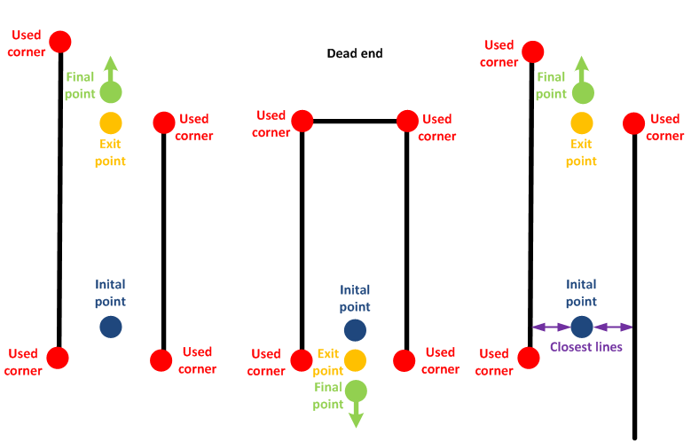
The corridor is the most difficult to handle crossing type. The lines parallel to Pico are the initial guess of the direction. If only one parallel line is found using corner detection, another method is used. All lines are cut is segments and the closest three lines are found. Two of these closest lines should be parallel to Pico and determine the direction. | |||
The direction of the lines is rotated if the lines are pointed backwards and then averaged. Here the correctness of the direction is of higher importance since larger distances may be traveled. Then it is checked whether the endpoints of the lines parallel to Pico are not part of the same line. If this is the case, a dead-end is found. Then the angle is changed 180 degrees. | |||
Then the distance to the shortest end of a line in front is determined. This distance is a little bit increased and added in the found direction to the current position. | |||
[[File:dead end path.png|300px|center]] | |||
===improvements=== | |||
An improvement would be to also detect whether Pico has left the maze. If no straight lines are visible close, the maze is solved and Pico should stop driving and start celebrating. | |||
It would be more robust to define the end angle absolute and not as a function of the old angle to avoid cumulative errors. The ‘old angle’ can then be determined with the direction of the walls parallel to Pico. | |||
Another improvement would be if more than two end points are found within one quadrant, to take a closer look at these points. Probably the wall consists of a single block and the two furthest points can be left unused in the path planning. | |||
==Follow the line== | |||
This algorithm is relatively simple. It follows the path which is in the middle of the corridor. An absolute position is used to navigate with a simple controller to the end point of the line. | |||
[[File:follow line1.png|300px|center]] | |||
The main idea is visible in the figure above. The line follower receives a path and a global position. The line follower drives to the end of the line if the shortest distance to the line stays within a margin. This margin is an absolute value since in this algorithm the corridor width is unknown. Otherwise it will first drive back to the line and then again to the end. If the end is reached within a certain margin and the odometry angle is matched to the angle form the path within a certain margin, a new path is requested from the ‘create path’ node. | |||
If Pico has to drive back a few lines, the line follower is able to follow these lines sequentially. The same position margin is used to switch to the next line. The angle is only matched at the last end point of the path of lines. | |||
The rotation rate is proportional to the difference between the odometry and the angle that has to be made to reach the end point from the current position. The velocity is inversely proportional to the rotation rate. If Pico deviates from the line, the rotation rate increases. This causes the forward velocity to drop resulting in an increased effect on the rotation. | |||
If the rotation rate reaches a certain value, the velocity is put to zero. This also prevents problems if a dead-end is found. Pico will first turn and will only start to drive if it is facing the direction of the end point. | |||
The velocity is also scaled with the distance to the end point. This prevents overshoot. | |||
The found velocity and rotation rate are sent to the ‘wall avoidance’ node which probably does not need to the change these values. | |||
This controller could probably be improved, but this is not done since it is not tested and its performance with this controller is unknown. Maybe it is also possible to tune the margins with the corridor width, but at this point, the corridor width is not sent along with the path. | |||
==Program evaluation== | |||
In the end, the mapping and navigation software was not used in the maze competition. A week prior to the competition, the implementation of the mapping and localization was not behaving correctly. Therefore, the low level program was developed in the last week to be sure that there was a backup. Debugging the SLAM algorithm was not finished at the time of the maze competition, so it could not be used. | |||
Latest revision as of 20:53, 22 May 2014
Group Name
Team Picobello
Group Members
| Name: | Student id: | Email: |
| Pepijn Smits | 0651350 | p [dot] smits [dot] 1 [at] student [dot] tue [dot] nl |
| Sanne Janssen | 0657513 | s [dot] e [dot] m [dot] janssen [at] student [dot] tue [dot] nl |
| Rokus Ottervanger | 0650019 | r [dot] a [dot] ottervanger [at] student [dot] tue [dot] nl |
| Tim Korssen | 0649843 | t [dot] korssen [at] student [dot] tue [dot] nl |
Introduction
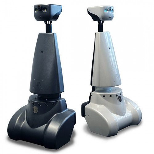
Nowadays, many human tasks have been taken over by robots. Robot motion control and embedded motion control in the future allow us to use robots for many purposes, such as health care. The (humanoid) robots therefore have to be modeled such that they can adapt to any sudden situation.
The goal of this project is to get the real-time concepts in embedded software design operational. This wiki page reviews the design choices that have been made for programming Jazz robot Pico. Pico is programmed to navigate fully autonomously through a maze, without any user intervention.
The wiki contains three different programs. The first program was used for the corridor competition. In this program the basic skills like avoiding collision with the walls, finding corners and turning are implemented.
After the corridor competition, a new design strategy was adopted. The second program consists of a low level code, namely a wall follower. By keeping the right wall at a fixed distance from Pico, a fairly simple, but robust code will guide Pico through the maze.
Besides this wall follower strategy, a high level approach was used. This maze solving program uses wall (line) detection to build a navigation map, which Pico uses to create and follow path lines to solve the maze. To update the position of Pico, the odometry information, local and global maps are used.
The latter two programs use Pico’s camera to detect arrows in the maze that point Pico in the right direction.
Data processing
Pico outputs a lot of sensordata. Most of the data needs to be preprocessed for use the maze-solving algorithm. The odometry data, laserscandata and imagedata are discussed below.
Odometry data
One of the incoming data types is the odometry. The odometry information is based on the angular positions of the robot wheels. These angular positions are converted into a position based on a Cartesian odometry system, which gives the position and orientation of Pico, relative to its starting point. For the navigation software of Pico, only the x,y-position and [math]\displaystyle{ \theta }[/math]-orientation are of interest.
Due to slip of the wheels, the odometry information is never fully accurate. Therefore the odometry is only used as initial guess in the navigating map-based software. For accurate localization, it always needs to be corrected.
This correction is based on the deviation vector obtained from the map updater. This deviation vector gives the (x,y,θ)-shift that is used to fit the local map onto the global map and therefore represent the error in the odometry. Because of the necessary amount of communication between the parts of the software that create the global map and the part that keeps track of the accurate position, these parts are programmed together in one node. This node essentially runs a custom SLAM (Simultaneous Localization and Mapping) algorithm.
Laserscan data
To reduce measurement noise and faulty measurements the laser data is filtered. Noise is reduced by implementing a Gaussian filter, which smoothens each data point over eight other data points.
[math]\displaystyle{ G(x)=\frac{1}{\sqrt{\sigma \pi}}e^{\frac{-x^2}{2 \sigma^2}} }[/math] with [math]\displaystyle{ \sigma = 2.0 }[/math]
Faulty measurements are eliminated in three different ways. First data points which deviate a lot from their neighbors are ignored in the Gaussian filter so that the filter does not close openings. When ignoring data points the Gaussian is normalized based on the used points.
Secondly the first and last 15 data points are ignored, decreasing the angle of view by 7.5 degrees at each side, but preventing the robot to measure itself. At last, only data points are used which are between a certain range, not only to prevent measuring the robot itself, but also to eliminate outliers.
Arrow detection
Binary image
From a full color camera image we want to determine whether there is an arrow and to determine its direction. Because this full color camera image is too complex to process, we transform it into a binary image. Since the arrows used in the competition are red, everything that is red (with a certain margin) is made white and the remaining is set as black.
Canny edge detection
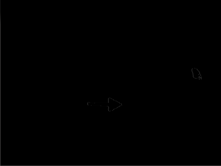
Next edges are detected with a canny edge detection algorithm from openCV. This algorithm uses a Gaussian filter to reduce noise, similar to the one explained above. But it also uses the gradient of this Gaussian filter. At and edge there is a very strong transition from white to black, resulting in an extreme value in the gradient. So by thresholding the gradient, edges can be detected.
Find contours
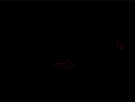
The binary image from the canny edge detection is used as input in the FindContours function from openCV. This function finds contours by connecting nearby points, giving a vector of contours as output. Each contour consists of a vectors filled with points.
Arrow detection
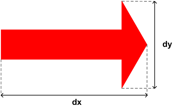
Finally the image is processed so that we can start detecting arrows. Arrows are detected in two steps. First the ratio of the height and the width of each contour is determined, to see if the contour can be an arrow, see figure 1. The arrow used in the competition has a ratio of 2.9, with a lower and upper bound, this results in: [math]\displaystyle{ 2.4 \lt \frac{dx}{dy} \lt 3.4 }[/math]
Next if a contour can be an arrow, the direction is investigated. This is done by determining the ratio of dx_right and dx_left, see figure 2. If the largest width (dy) is shifted towards the right dx_left > dx_right and the other way around. With some lower and upper bound this results into:
Right arrow if:
- [math]\displaystyle{ dx_{left} \gt \frac{5}{4} dx_{right} }[/math]
Left arrow if:
- [math]\displaystyle{ dx_{left} \lt \frac{4}{5} dx_{right} }[/math]
No arrow if:
- [math]\displaystyle{ \frac{4}{5} dx_{right} \lt = dx_{left} \lt = \frac{5}{4} dx_{right} }[/math]
If the largest width is in between the margins, the contour cannot be an arrow and is treated as such. This may not be the most robust way to detect an arrow, but during the tests it seemed to work just fine. A few other methods that can be used or combined to make the arrow detection more robust are circularity, shape matching, matching of moments or finding lines with the Hough transform.
 |
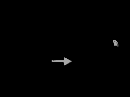 |
 |
 |
 |
Program 1: Corridor Challenge solver
Wall avoidance
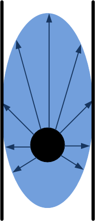
The function ‘wall_avoidance’ has the simple function of preventing collisions. It therefore overrules the determined velocity and rotation if an object is very close.
The function calculates a region in which no objects are allowed. This region is elliptically shaped and its parameters are velocity and rotation rate dependent. This makes it possible to drive near objects if the velocity is low, for example when driving in a narrow corridor.
This function could be improved by not only using the rotation rate but also the rotation direction. Now Pico may stop when driving to the right if an object is to the left. The ellipse should then consist of more than two parameters.
.
Edge detection
For the corridor competition, Pico should first be able to detect an outside corner (see figure 9). To detect corners, the laser range data is used.
The robot searches left and right for large differences in wall distance. If the length ratio between two neighboring ranges exceeds a certain threshold, the position (1) of the outside corner is saved. Also the side of the corridor is set to left or right. If the first corner has been found, Pico searches at this side for other corners. This search algorithm starts at the first corner and checks for the shortest laser range distance. This coordinate is saved as second edge position (see figure 10). The coordinates of the edges are sent to the make turn function, which controls Pico’s movement.
If Pico is past the first corner, the first algorithm explained above cannot recognize this first corner anymore. To avoid problems, the second algorithm is activated for both the first and last corner (see figure 11).
 |
 |
 |
Turning into the corridor
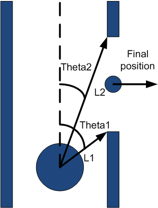
If the first corner is passed, a boolean is set to true and the centering algorithm is replaced by the algorithm used to make a turn. This algorithm uses the two corners of the side exit determined by the corner detection algorithm.
First it drives a little towards the side exit but prevents a collision with the first corner. If the middle of the side exit is reached, L1 = L2 in figure 12, Pico is turned until both angles to the corners are equal, Theta1 = Theta2. It then drives in the exit while keeping the difference between the distances to the corners within a margin. If the absolute values of the angles to the corners are both larger than 90 degrees, the make turn algorithm is switched off and the centering algorithm is switched on again.
The algorithm could be improved by not only using the distances to the corners but also preventing coming to close to the other wall of the corridor. This is not a big problem since the wall avoidance algorithm prevents collisions.
.
Centering algorithm
This algorithm uses the shortest length to left and right and the corresponding angle. These properties are derived in the function ‘detectWalls’ and put together in one variable. Its output is a forward velocity and a rotation rate.
First the current corridor width is determined by summing up the shortest distances to the left and the right. This sum is wrong when a side exit is reached, but this is not a problem since a different function is used to make the turn.
If the distance to one of the sides is smaller than one third of the corridor width, it is determined if Pico is facing the wall or the middle of the corridor, see the red area in figure 13. If it is facing the wall it is turned back without driving forward, if it is facing the middle, it drives with a velocity of 0.2.
If Pico is in the middle third if the corridor, it also drives forward with a velocity of 0.2, see green area in figure 13.
The function could be improved by determining the angle that has to be made to face the right direction. This angle should not be used as the rotation rate, but the odometry should be used to determine if the preferred angle is reached.
Another improvement would be a better controller, which also steers if Pico is still in the middle part of the corridor. This was not implemented since in this stadium the function wall_avoidence was still very basic and could not handle driving and steering well.
.
Program structure

This program has a single node structure. All functions are defined internally in a so called ‘awesome node’. The wall avoidance has the highest priority in the node to avoid wall collision. The second most important function is the centering algorithm. if the edge detection has detected a side corridor, the turning algorithm is activated. A schematic view is shown in figure 14.
.
Program evaluation
During the corridor competition, the program was fixed, but some bugs came up. The functions stay in middle and wall avoidance worked well, but during the last simulations before the corridor competition, the corner detection showed some undesired results.
The first and second corners are detected correctly. While turning however, Pico starts to recognize an outside corner at the end of the corridor, as depicted in figure 15. This third corner confuses the program, because the turning algorithm now questions which corners to use as a reference. Due to this unexpected corner, Pico was not able to solve the corridor competition. Therefore two new strategies were developed to win the upcoming competition: solving the maze. The wall follower and high-level maze solving program.

Program 2: Wall Follower
Structure
The wall follower is constructed as shown in figure 16. First the laserdata is used for wall-avoidance as explained above and dead-end detection. Also the cameradata is used to detect arrows. Based on these three modules, the priority algorithm decides which action to take and is more or less the ‘brain’ of the program. Depending on the desires of the priority algorithm, the controller makes sure Pico either follows the right wall or makes a left turn.
Dead end detection
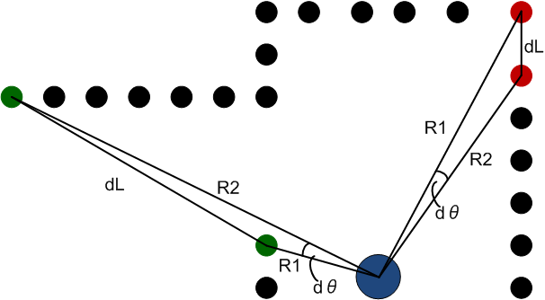
The main reason for dead-end detection is to make sure Pico does not drive into corridors without an exit or crossing at the end. The main idea is that if dead-ends can be detected, Pico returns immediately, which can save a lot of time.
Dead-ends are detected by closed contours in the filtered laser data. To find closed contours the distance (dL) between two subsequent data points is calculated with the cosine rule:
[math]\displaystyle{ dL = \sqrt{R_1^2+R_2^2-2R_1R_2cos(d\theta)} }[/math]
If two points are inside a closed contour, the distance between those points is small, see the red dots in figure 17. While they are not inside a closed contour the distance is large, see the green dots in the same figure. To determine whether the points are in- or outside a closed contour we use a threshold, [math]\displaystyle{ dL \lt dL_{max} }[/math].
Finally we say there is a dead-end, if the contour is closed for a certain range of points. Testing confirmed that a range of -60 to 60 degrees ensures that Pico does not only correctly detect dead-ends, but also detect them from a reasonable distance.
If a dead-end is detected the robot turns left, until it finds an opening within the -60 to 60 degrees ranges and then continues following the right wall.
Priority algorithm
There is a simple decision making algorithm that can decide to follow the right wall, turn left or stop. This is done by checking the states of different modules and their desires. The wall follower always wants to follow the right wall, except when there is a dead-end or an arrow to the left. In these cases the robot will turn left. Arrows to the right are ignored, since the robot already wants to go that way. Finally if the robot is too close to a wall the wall avoidance wants Pico to stop. This results in the following priority: Wall avoidance > Arrow detection > Dead-end detection > Wall follower
Controller

The controller is a simple proportional controller, based upon a few essential values, defined in figure 18
The essential values are the closest distance to the wall and their corresponding angles, defined in three different areas.
- Left: -130 until -10 degrees.
- Front: -30 until 30 degrees.
- Right: 30 until 130 degrees.
The wall follower always wants to keep [math]\displaystyle{ L_{right} }[/math] at a distance (d) of the wall, see figure 18
The controller sends an angular velocity ([math]\displaystyle{ \dot{\theta} }[/math]) to Pico, which is proportional to the difference between this setpoint and the minimal distance to the right wall. So
- [math]\displaystyle{ \dot{\theta}\sim L_{right}{-}d }[/math]
To make sure that the robot drives as straight as possible, the angle towards the closest distance at the right wall ([math]\displaystyle{ \theta_{right} }[/math]) is kept at 90 degrees. Also
- [math]\displaystyle{ \dot{\theta}\sim\theta_{right}{-}\pi/2 }[/math]
The linear velocity (v) is also controlled proportionally. If [math]\displaystyle{ L_{front} }[/math] is large, the path is clear and meaning it is fairly safe to drive fast. So
- [math]\displaystyle{ \mathbf{v}\sim L_{front} }[/math]
Both linear and angular velocity are limited by 0.2 and 0.7 respectively.
Program evaluation
A wall-follower is a fairly simple, but very robust program. It also benefits from dead-end and arrow detection; two features which both highly increase the performance. On the other hand, the simplicity of the program will eventually prevent the program from becoming highly intelligent. The lack of a map makes position determination, decision making and complex maze configurations hard to deal with. This is the program we used during the final competition, which resulted in the first place.
Program 3: Map based strategy
Program Structure and introduction
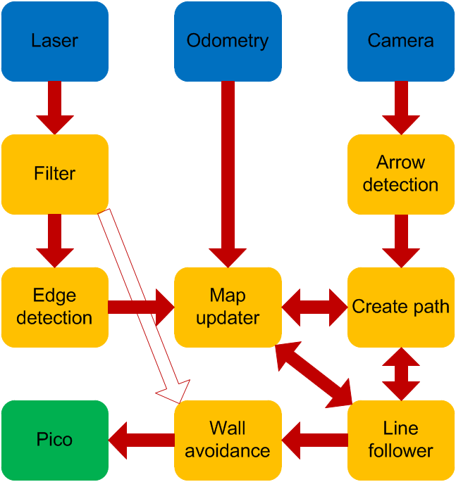
The wall following code is effective and robust, but a more challenging code was created. Here a total map of the maze is created and used to determine its path.
The laser data is filtered with the aforementioned Gaussian filter.
A local map is created from the laser data only. This results in lines representing the visible walls which are then sent to the map updater node. Then the local map and odometry are updated with an optimization algorithm to match the global map. The global map is updated and visualized together with the driven path.
This map is then sent to the node ‘create path’. This function also receives an arrow direction if an arrow is detected. If a service is asked from the ‘Line follower’ the end point of the last path is reached and a new one has to be sent back. This path consists of a line with an end point and an absolute angle that has to be matched with the odometry at the end of the line.
It is also possible to do this path planning with the local map, but then it is not possible to create a path going back when a dead-end is found. The global map consists of many optimization steps and is therefore much more reliable than the local map.
The line follower receives the new path and a global position. The line follower drives to the end of the line if the shortest distance to the line stays within a margin. Otherwise it will first drive back to the line and then again to the end.
Then the earlier described ‘wall avoidance’ node checks if no objects are close and sends the velocity and rotation rate to Pico.
The main advantage of this map based navigation is that arrows can be used smartly and the path planning allows for feed forward where the wall follower only uses feedback. The path planning algorithm can be improved for creating smooth corners and determining the path before the end of the line is reached. In this way to the total maze can be driven with the maximum velocity of 0.2.
Local map creation
To create a useful and efficiently containable map, the laser data must be reduced to the essential information it contains. Since the walls scanned by the laser data are in good approximation straight, these can be represented by line segments. Before any search for lines is done, the laser data is filtered with the specialized Gaussian filter (#Laserscan data).
Local map To obtain the line segments, the approach proposed by group 5 of 2012 ([[1]]) is adopted. The method is implemented as follows.
create a line between point 1 and point 2 of the LRF data (LINE class)
l = current line (defined by first two points)

FOR all data points
p = current point
   	s = current new line segment (defined by end of current line and current point)
nFaulty = current number of points found that do not belong to s

IF ( nFaulty < n_max AND angle between l and s < angle_max AND length of s < length_max)
// Point is good and can be added to the line
replace end point of l by current point
nFaulty := 0
ELSE IF ( nFaulty >= n_max )
	add current line to array of lines (map)
	IF ( length of s > length_max )
		// There is a jump in the laser data, so an outer corner point is found
		//initiate new current line with
start point := saved first faulty point
end point := current point
ELSE
	// The angle was too large, so an inner corner point is found
	// initiate new current line with
	start point := end point of old current line
	end point := current point
END
ELSE
IF (first faulty point found)
save current point to start potential new line from
END
		nFaulty ++
	END
END
After this original setup, an extra if statement was added to keep the algorithm from adding line segments that are too long to a line (possible if there are two jumps in laser data right subsequent of each other.
Implementing this routine and testing it showed that the resulting number of lines is too high. Especially the laser data near the robot is relatively noisy. This is most likely due to the fact that the absolute error in laser range data stays about equal, such that the relative error on small measurements is relatively large. Also the points near the robot are relatively close together (order of millimeters), so that the error in the laser data quickly results in a large angle between the current line and the to-be-added line segment. The algorithm recognizes this as being an inner corner, so it does not add the line segment to the current line.
To deal with this, an extra filter is implemented over the lines, which combines lines if their difference in angle is within a certain range which is narrower than used in the original algorithm. Also short lines are combined with one of their direct neighbours. This way, short lines that occur due to noise are filtered out and corners are sharpened. The additional filters reduce the number of lines found from around 60 to less than 10.
Global map
For navigation purposes, a global map is desired. This global map can be built out of the local maps from each time step. However, these local maps are saved in a vector format with the robot fixed reference frame as a base. The global map needs to be defined in a global perspective. Hereto the local map is transformed to a global vector base. Additionally, the position of the robot in the map is required. This is however a nice byproduct of the process of creating a map. The noisy and error sensitive odometry information can be enhanced using the translation and rotation necessary to fit the local map to the global map.
Firstly, the global vector base must be defined, this can be done using the robot’s initial position (at the start of the program). This position and orientation is chosen as the (x,y,theta) = (0,0,0) point of the global map. Next, the local map created by the robot needs to be translated and rotated to the global base. This can be done by using an estimation of the robot’s position given by the odometry information (#Odometry data). Every point in the local map can be transformed to a point in the global map using the following transformation:
[math]\displaystyle{ \mathbf{x_{global}} = \begin{bmatrix}
cos(\theta) & -sin(\theta) \\
sin(\theta) & cos(\theta) \\
\end{bmatrix}. \begin{bmatrix}
x_{local} \\
y_{local} \\
\end{bmatrix}+\begin{bmatrix}
x_{robot} \\
y_{robot} \\
\end{bmatrix}. }[/math]
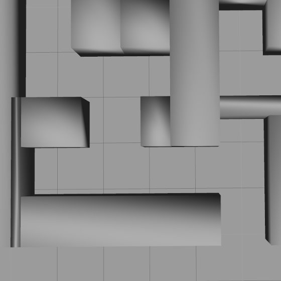
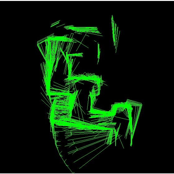
where \theta is the orientation of the robot in the global system, the local coordinates are the coordinates of a point with respect to the robot fixed frame and the robot coordinates depict the robot’s position in the global frame of reference. This creates a local map in the coordinate system of the global map. This map can now be added to the global map. Using this method it is already possible for a human to get some understanding of the layout of the maze. An example can be found in figures 20 and 21.
To create a better map, it is possible to start by replacing lines in the global map by their corresponding lines in the local map. However, as can be seen in figures 20 and 21, the lines drift off as the robot drives through the maze. This can be attributed to the accumulating error in the odometry information.
The error can be accounted for by fitting the new local map to the old global map. To do this, first the common points must be found. A brute-force approach is acceptable since the number of corner points in the maze is limited. Points are said to be common if their coordinates are within a predefined range of each other. Additionally, each point is the end point to a line, the angle of the line in the local map should be within a certain range from the angle in the global map.
Optimization problem When the common points are found, the points in the local map can be fitted to the points in the global map by minimizing their respective distances. The distance between two corresponding points i can be expressed as
[math]\displaystyle{ d_{i}=\sqrt{(x_{ig}-x_{il})^2+(y_{ig}-y_{il})^2} }[/math]
[math]\displaystyle{ d_{i}=\frac{1}{\sqrt{\sigma \pi}}e^{\frac{-x^2}{2 \sigma^2}} }[/math] with [math]\displaystyle{ \sigma = 2.0 }[/math]
where subscript [math]\displaystyle{ g }[/math] means global and [math]\displaystyle{ l }[/math] means local. The local map can then be perturbed by a vector [math]\displaystyle{ r_{dif}=(x_{dif},y_{dif},\theta_{dif}) }[/math] such that
[math]\displaystyle{ x_{il} = (1+\cos\theta_{dif})x_{il,old} + x_{dif} }[/math]
[math]\displaystyle{ y_{il} = (1+\sin\theta_{dif})y_{il,old} + y_{dif} }[/math]
where subscript [math]\displaystyle{ il, old }[/math] il,old means the [math]\displaystyle{ i }[/math]’th point in the list of common points found in the local map, and [math]\displaystyle{ il }[/math] is the perturbed point.
Using above equations for all common points one obtains a vector of distances. Now to obtain a scalar value to optimize, the obvious way is to use the Euclidean norm. It is however computationally cheaper not to determine the square root of the sum of squares. So the objective function becomes
[math]\displaystyle{ f(x_{dif},y_{dif},\theta_{dif}) = \sum_{i = 0}^{k}(x_{ig}-x_{il, old}(1+\cos\theta_dif)-x_{dif})^2+(y_{ig}-y_{il, old}(1+\sin\theta_{dif})-y_{dif})^2, }[/math]
where [math]\displaystyle{ k }[/math] is the number of common points found. Using any norm has the advantage that the resulting function is convex. This means that any minimum is a global minimum and Newton’s method for optimization can be used to obtain this minimum.
Implementation of Newton’s method
http://en.wikipedia.org/wiki/Newton's_method http://en.wikipedia.org/wiki/File:NewtonIteration_Ani.gif Newton’s method can be used to find minima of a twice differentiable function by calculating the roots of the derivative. In this case, the objective function is a function of three variables. This means the vector form of Newton’s method is used. Newton’s method is implemented as
[math]\displaystyle{ x_{n+1}=x_{n}-[Hf(x_{n})]^{-1}\nabla f(x_n). }[/math]
The gradient vector and Hessian matrix are calculated by hand. The original coordinates of the points in the local and the global map are coefficients in these. However, calculating the inverse of the Hessian is impossible beforehand because it is the sum of an undetermined number of terms (dependent on the number of common points in the local and the global map). Calculating the inverse of the Hessian is computationally expensive. A common way to deal with this is to calculate
[math]\displaystyle{ p_{n}=[Hf(x_{n})]^{-1}\nabla f(x_n) }[/math]
solving
[math]\displaystyle{ \nabla f(x_n)=[Hf(x_{n})] p_{n}. }[/math]
This is a linear system, which can be solved much more quickly.
Using an appropriate stopping condition, only a few (order 10) iterations are needed to produce an accurate value for the minimum argument.
Path creator
This node uses the global map and the presence and direction of arrows. It consists of the following five steps:
1) Determining the closest points and their positions
2) Determining the crossing type
3) Checking for arrows
4) Checking for driven path
5) Creating the path
6) Send and save the path
Its preferred direction is to the right. So, just like the wall follower, if nothing special happens, the robot will always turn to the right.
Determine the closest points and their positions
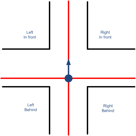
All start and end points of the lines of the global map are checked and put in a vector if they are closer than one corridor width. This vector is then split up in four vectors representing the four quadrants relative to Pico (See figure 22). Also two vectors are made of the lines that are parallel. With this information it is possible to distinguish all but two crossing types and create all of the paths. This is possible since the angular position is also determined by the previous path and therefore known.
Determine the crossing point
Seven different crossing types can be distinguished including the corridor:
1. 3 exits. End points in all quadrants.
2. 2 exits; left and strait on. End points in the two left quadrants.
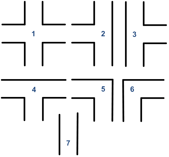
3. 2 exits; right and strait on. End points in the two right quadrants.
4. 2 exits; left and right. *End points in the two quadrants behind.
5. 1 exit; left. End points in the quadrant on the left behind and on the right in front.
6. 1 exit; right. End points in the quadrant on the right behind and on the left in front.
7. 1 exit; straight (corridor). *End points in the two quadrants behind, or only points in the quadrant left behind, or only points in the quadrant right behind.
.* It is not possible to know if a corridor or a T-junction is reached. This is then done by checking whether all start points belonging to the lines with their end points on the crossing are behind Pico. If this is the case a T-junction is reached.
checking for arrows

If an arrow is found, the path is towards the arrow. The arrow is then followed if the crossing with the arrows (probably T-junction) is reached.
Checking for driven path
This function is not actually needed if the robot always turns to the right, but it increases the robustness of the program. Due to this algorithm a wrongly identified arrow does not need to be fatal.
If a crossing is reached and one or two of the exits are already visited, the path will go in the direction that is left or turn around. If it has to turn around (also at a dead-end) the entire saved path is checked for the first possibility to deviate from it. This is then sent in a vector of lines and a direction to the line follower.
If a different exit has to be chosen than the first right, this is done by changing the determined crossing type. For example, if a crossing with three exits is reached and the front and right exit are already visited, Pico should go left. This is done by removing the found end points of lines on the quadrants in front on the left and behind on the right.
Creating the path
The starting point of a path is always the end point of the previous path. Subsequently the exit point and the angle with respect to the last angle sent are defined. In this direction a small extra distance is added. This ensures that the crossing has been passed.
If possible, the exit is found by averaging between two points at the edges of the exit.
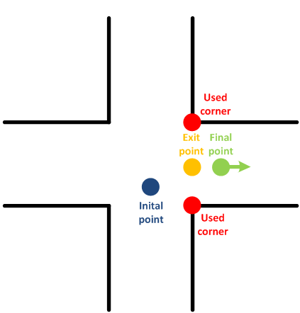 |
 |
When this is not possible a ‘new point’ is defined. This is done with the corridor width and the direction of the walls alongside Pico. Sometimes this direction needs to be turned first. This new point and one of the old points is averaged to find the exit point.
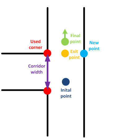 |
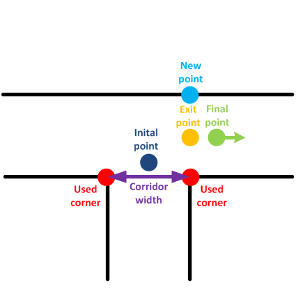 |
The crossing types with only one exit are treated differently. For the two corners a line is defined between the corner points. This line is turned 90 degrees and its length is divided by two. This new line is then added to the current position; this defines the exit of the crossing.
 |
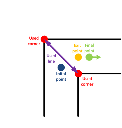 |
The corridor is the most difficult to handle crossing type. The lines parallel to Pico are the initial guess of the direction. If only one parallel line is found using corner detection, another method is used. All lines are cut is segments and the closest three lines are found. Two of these closest lines should be parallel to Pico and determine the direction. The direction of the lines is rotated if the lines are pointed backwards and then averaged. Here the correctness of the direction is of higher importance since larger distances may be traveled. Then it is checked whether the endpoints of the lines parallel to Pico are not part of the same line. If this is the case, a dead-end is found. Then the angle is changed 180 degrees.
Then the distance to the shortest end of a line in front is determined. This distance is a little bit increased and added in the found direction to the current position.
improvements
An improvement would be to also detect whether Pico has left the maze. If no straight lines are visible close, the maze is solved and Pico should stop driving and start celebrating. It would be more robust to define the end angle absolute and not as a function of the old angle to avoid cumulative errors. The ‘old angle’ can then be determined with the direction of the walls parallel to Pico.
Another improvement would be if more than two end points are found within one quadrant, to take a closer look at these points. Probably the wall consists of a single block and the two furthest points can be left unused in the path planning.
Follow the line
This algorithm is relatively simple. It follows the path which is in the middle of the corridor. An absolute position is used to navigate with a simple controller to the end point of the line.
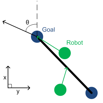
The main idea is visible in the figure above. The line follower receives a path and a global position. The line follower drives to the end of the line if the shortest distance to the line stays within a margin. This margin is an absolute value since in this algorithm the corridor width is unknown. Otherwise it will first drive back to the line and then again to the end. If the end is reached within a certain margin and the odometry angle is matched to the angle form the path within a certain margin, a new path is requested from the ‘create path’ node.
If Pico has to drive back a few lines, the line follower is able to follow these lines sequentially. The same position margin is used to switch to the next line. The angle is only matched at the last end point of the path of lines. The rotation rate is proportional to the difference between the odometry and the angle that has to be made to reach the end point from the current position. The velocity is inversely proportional to the rotation rate. If Pico deviates from the line, the rotation rate increases. This causes the forward velocity to drop resulting in an increased effect on the rotation.
If the rotation rate reaches a certain value, the velocity is put to zero. This also prevents problems if a dead-end is found. Pico will first turn and will only start to drive if it is facing the direction of the end point. The velocity is also scaled with the distance to the end point. This prevents overshoot. The found velocity and rotation rate are sent to the ‘wall avoidance’ node which probably does not need to the change these values. This controller could probably be improved, but this is not done since it is not tested and its performance with this controller is unknown. Maybe it is also possible to tune the margins with the corridor width, but at this point, the corridor width is not sent along with the path.
Program evaluation
In the end, the mapping and navigation software was not used in the maze competition. A week prior to the competition, the implementation of the mapping and localization was not behaving correctly. Therefore, the low level program was developed in the last week to be sure that there was a backup. Debugging the SLAM algorithm was not finished at the time of the maze competition, so it could not be used.