Embedded Motion Control 2017 Group 10: Difference between revisions
| (56 intermediate revisions by 3 users not shown) | |||
| Line 97: | Line 97: | ||
==''Interface''== | ==''Interface''== | ||
The interfaces between functions are shown in Figure 3. Here the functions are devided into: Tasks, Skills, | The interfaces between functions are shown in Figure 3. Here the functions are devided into: Tasks, Skills, Motions and the World Model. The world model contains the functions that are used to keep track of Pico's surrounding. Tasks contains the functions on the highest level where the robot decides what it is going to do, like solve the maze. The skill block consists of all functions that make the robot perform lower level tasks such that the high level objective can be achieved. The motion block does the low level operations that make the skill functions work. | ||
[[File:Interfaces v1.png|thumb|center|600px|alt=interface diagram group 10|Figure 3: Interface overview of all functions needed by Pico to solve the maze and corridor challenge.]] | [[File:Interfaces v1.png|thumb|center|600px|alt=interface diagram group 10|Figure 3: Interface overview of all functions needed by Pico to solve the maze and corridor challenge.]] | ||
| Line 103: | Line 103: | ||
==''Moving and cornering''== | ==''Moving and cornering''== | ||
A couple of things are used in order for Pico to move through the corridor and make a corner. The first thing is a potential field. This creates an artificial bubble around Pico which repels it from objects that get too close. The second thing that allows Pico to make the corner in the corridor is its corner detection. This corner detection analyses the data from Pico's laser sensor and finds the corners of the corridor. When Pico approaches a corner on either side of the corridor, a reference point is placed beyond this corner in the middle of the hallway Pico should turn into. An attracting force is created that pulls Pico straight towards this reference point. Of course Pico can't go straight to this reference point since part of the wall is in the way and Pico is pushed from this by the potential field (see | A couple of things are used in order for Pico to move through the corridor and make a corner. The first thing is a potential field. This creates an artificial bubble around Pico which repels it from objects that get too close. The second thing that allows Pico to make the corner in the corridor is its corner detection. This corner detection analyses the data from Pico's laser sensor and finds the corners of the corridor. When Pico approaches a corner on either side of the corridor, a reference point is placed beyond this corner in the middle of the hallway Pico should turn into. An attracting force is created that pulls Pico straight towards this reference point. Of course Pico can't go straight to this reference point since part of the wall is in the way and Pico is pushed from this by the potential field (see Figure 4). This combination of attraction and repulsion creates a curved path around the corner and into the exit of the corridor. Pico keeps cornering until either the odometry has detected that a turn of more than 1/2 Pi radians has been made or until the point around which Pico is cornering has been lost out of sight. As shown in the corridor challenge result video below, a drunk Pico makes a beautiful turn to exit the corridor. In the two following sections the inner workings of the potential field and the corner detection are explained in greater detail. | ||
[[File:Cornering_group_10_2017.png|thumb|center|500px|alt=effective speed group 10|Figure | [[File:Cornering_group_10_2017.png|thumb|center|500px|alt=effective speed group 10|Figure 4: When a corner is detected (yellow dot), a reference point is placed a bit further in the middle of the hallway. Pico is drawn towards this reference point by a vector that points straight at it. This vector is combined with Picos potential field to create a smooth path around the corner (blue line).]] | ||
==''Potential field''== | ==''Potential field''== | ||
In order for Pico to safely manoeuvre through the corridor, a potential field is implemented. This potential field will push Pico away from walls with a force that gets bigger the closer Pico gets to a wall. The size and direction of this force is calculated based on the data gained from the laser sensor. First, the length of all 1000 laser lines is inverted and the angle of each line is shifted over an angle of Pi radians. This creates vectors that point away from obstacles with a force that increases the closer an obstacle is to Pico. After that, all converted vectors are split into x and y segments which are summed up and recombined to create a single vector pointing away from any obstacles. The size of the resulting vector equals the force, and thus speed, with which Pico is pushed away from the obstacles. In order to make the behaviour of Pico more predictable the size of the resulting vector is normalized and rescaled based on the closest object at a later point. Rescaling all vectors that influence Picos movements (potential field and reference point from previous section) based on the distance to the nearest object creates a clear overview of how these different forces interact and make Pico move. Figure 5 visualizes the potential field. | |||
In order for Pico to safely manoeuvre through the corridor, a potential field is implemented. This potential field will push Pico away from walls with a force that gets bigger the closer Pico gets to a wall. The size and direction of this force is calculated based on the data gained from the laser sensor. First, the length of all 1000 laser lines is inverted and the angle of each line is shifted over an angle of Pi radians. This creates vectors that point away from obstacles with a force that increases the closer an obstacle is to Pico. After that, all converted vectors are split into x and y segments which are summed up and recombined to create a single vector pointing away from any obstacles. The size of the resulting vector equals the force, and thus speed, with which Pico is pushed away from the obstacles. In order to make the behaviour of Pico more predictable the size of the resulting vector is normalized and rescaled based on the closest object at a later point. Rescaling all vectors that influence Picos movements based on the distance to the nearest object creates a clear overview of how these different forces interact and make Pico move. | |||
[[File:Potential_field_group_10_2017.png|thumb|center|500px|alt=effective speed group 10|Figure | [[File:Potential_field_group_10_2017.png|thumb|center|500px|alt=effective speed group 10|Figure 5: The laser data from Picos laser sensor is used to make a potential field. The length of every laser line is inverted and shifted over an angle of Pi radians. The resulting vectors are summed up to create a single vector which points in the direction of the most open space.]] | ||
=='' Corner detection''== | =='' Corner detection''== | ||
To detect corners and walls the Split and | To detect corners and walls the 'Split and Merge' algorithm is used on the laser data. This algorithm contains the following procedure: | ||
* 1. Laser data is transformed | * 1. Laser data is transformed into x and y coordinates | ||
* 2. | * 2. Laser data points will grouped into segments | ||
* 3. Within each segment | * 3. Within each segment a line is drawn between the first and last point and the perpendicular distance between each other point and this line is checked | ||
* 4. If the maximum perpendicular | * 4. If the maximum perpendicular distance is above a set threshold (0.2 m), this point will be set as a vertex within this segment. | ||
* 5. Step 3 and 4 will be repeated until there are no new vertices are found. | * 5. Step 3 and 4 will be repeated until there are no new vertices are found. | ||
* 6. Within each segment a line will be defined using the least squire method. | * 6. Within each segment a line will be defined using the least squire method. | ||
* 7. If two lines are connected with each other, the intersection will be used to define the vertex. | * 7. If two lines are connected with each other, the intersection will be used to define the vertex. | ||
* 8. If there | * 8. If there a line has no further connections, the last point of the line will be set as an end point. | ||
These steps are visualized in the figure below: | These steps are visualized in the figure below: | ||
| Line 135: | Line 127: | ||
[[File:Split and merge resized.gif|center|alt=interface diagram group 10|Split and merge procedure.]] | [[File:Split and merge resized.gif|center|alt=interface diagram group 10|Split and merge procedure.]] | ||
To create a better and more stable fit of lines on the data, the standard 'Split and merge' algorithm has been expanded with a 'Least Square Method'. As can be seen in the first situation in the figure below, there is a wall left of Pico. Using the standard Least Squire Method, a line (yellow) is constructed where the error (purple) between the points and the line is minimized over the y axis. However, if there is a wall in front of pico, as shown in the second situation, the least squire method finds a line that is not equal to the orientation of the wall. This is because the standard method minimizes the error over the y axis. If the same procedure method is used over the y axis, as shown in the third situation, the found line has the same orientation as the wall. Therefore, the Least Square Method is extended so that the Least Square Solution over x or y axis is picked for which one the error is the smallest. | |||
[[File:Least squire method advanced2.png|thumb|center|700px|alt=function diagram group 10|Figure 6: Least square method for x and y axis.]] | |||
=='' Visualization corner detection''== | =='' Visualization corner detection''== | ||
In order to test the corner detection, a visualization is made based on the existing code from 'emc-viz'. With this visualization it is easier to see what pico observes. On the left in green dots, the raw laser data is shown. In the middle the result after the split and merge algorithm is applied. On the right the walls and corners are shown after removing false walls and applying the Least Square Method. From this GIF it is visible that the error on the edges and lines is reduced, and the results are more stable/robust. | |||
[[File:GIF visualisation corners group 10.gif|center|alt=interface diagram group 10|Visualisation corner detection; (from left to right) raw data, after split and merge, after Leas Squire Fitting.]] | [[File:GIF visualisation corners group 10.gif|center|alt=interface diagram group 10|Visualisation corner detection; (from left to right) raw data, after split and merge, after Leas Squire Fitting.]] | ||
| Line 195: | Line 143: | ||
='''The Maze Challenge'''= | ='''The Maze Challenge'''= | ||
== Final design== | == Final design== | ||
To solve the maze challenge there are designed individual parts, which will be explained in the next part. To manage these individual parts | To solve the maze challenge there are designed individual parts, which will be explained in the next part. To manage these individual parts the state machine shown in Figure 7 is needed. This state machine switches from one state to another based on the given outputs. The start state of the state machine is 'Go Straight', this is because the counter of the Plegde algorithm start at zero and Pico should not follow a wall in these conditions. Pico stays withing this state until it detects a wall in front of it. To do this it uses the function 'Detect wall'. This function simply checks the range of the front facing laser beams. If the detected range gets below a threshold, the state machine switches to the 'Follow wall' state. In order to move the robot straight ahead, the 'Go straight' state also has a function to move the robot. In order to prevent deadlocks in certain situations the robot always returns to the 'Follow wall' state after leaving another state. Before doing anything in the 'Follow wall' state, conditions are checked for dead ends and the pledge algorithm is updated. If a dead end is found the robot will switch to the 'Dead end' state. If the pledge counter is set to zero and no dead end is detected, the robot will enter the 'Go straight' state. | ||
Part of the maze challenge is to open a door which can be seen as a dead end because of the specifications of a door in the assignment. Attempting to open a door should therefor only be done when the robot finds itself near a dead end. Because of this, the 'Ring bell' functionality to open the door is located inside the 'Dead end' state. To get in the 'Dead end' state the 'Follow wall' state has a function called 'Dead end detection'. When this results in a positive outcome, the state machine switches to the 'Dead end' state. Once inside the 'Dead end' state the robot attempts to open the door by ringing a bell and waiting 5 seconds. This has two potential outcomes. Either the dead end had a door, or it didn't. The robot checks which outcome is the case by rerunning the 'Dead end detection' function. If it finds no dead end it means there was a door and it has been opened. The robot can now resume its wall following by returning to the 'Follow wall' state. If it still finds a dead end however, it means there was no door and the robot is simply located in a real dead end. To prevent a dead lock in which the robot keeps checking for dead ends and trying to open a door that isn't there, the robot enters the 'Exit dead end' state. In this state the robot will resume its normal wall following behavior, but without checking for dead ends. It will stay in this state until it has moved more than one meter away or turned more than 180 degrees from the position where it entered the state. When these conditions are met the robot will reenter the 'Follow wall' state. | |||
[[File:Group 10 State setup.png|thumb|center|800px|alt=state machine group 10|Figure 7: State machine]] | |||
With these four states and the individual functions, Pico should be capable of solving the maze challenge. The following sections will give in depth explanations of the functions that have not been explained before (Wall following, Pledge, Dead end detection). | |||
With these four states and the individual functions, Pico should be capable of solving the maze challenge. | |||
==Individual state machine functions== | ==Individual state machine functions== | ||
=== Wall following=== | === Wall following=== | ||
To implement the pledge based strategy it is necessary for Pico to be able to follow a wall in a robust manner. For this goal a wall following function has been implemented. This function makes use of some of the functionality of the corner detection explained earlier. This used part connects the individual laser dots and forms a single line that follows the overall direction of the wall (see Figure | To implement the pledge based strategy it is necessary for Pico to be able to follow a wall in a robust manner. For this goal a wall following function has been implemented. This function makes use of some of the functionality of the corner detection explained earlier. This used part connects the individual laser dots and forms a single line that follows the overall direction of the wall (see Figure 8). Based on this line a reference point at a fixed distance from the wall is set for the robot. Using a PD-controller, the robot is then moved to keep itself at this reference point. Another PD-controller is used to keep the difference between the angle of the wall and Pico close to zero. This causes Pico to drive parallel to the wall. The two PD-controllers are then combined with the potential field to make sure Pico never bumps into any walls. Finally, to move Pico forward, a fixed reference point is placed in front of it which moves it forward at maximum speed when no obstacles are detected. | ||
[[File:Wall_detection_group_10_2017.png|thumb|center|750px|alt=scalar image group 10|Figure | [[File:Wall_detection_group_10_2017.png|thumb|center|750px|alt=scalar image group 10|Figure 8: This image pictures Pico following a wall that makes a right turn. The black arrows and gray area dictate the region of the laser data that is used during the wall following. With functionality of the corner detection function explained earlier, a line is drawn through the laser points. Any points that lie further than 0.4 meters are discarded and not seen as part of the current wall. The orientation of the line is compared to that of Pico which results in the error <math>\alpha</math>. This error is used in the angle PD-controller to keep Pico parallel to the wall or, in this case, make Pico turn to follow the general direction of the detected wall. To keep Pico at a safe distance from the wall, a reference point is placed at 30 cm from the wall. Picos current distance from the wall is compared to this reference point which results in an error. This error is used in the other PD-controller to keep Pico at a set distance from the wall. There might be situations during turns or unknown environments where the line drawn through the wall gets placed in such a manner that the reference point causes Pico to collide with its environment. To prevent this from happening the PD-controllers are combined with the potential field.]] | ||
In order to balance the three different forces at work (PD-controllers, potential field, forward reference), each force is scaled based on the distance and position of to the closest object. When, for instance, no objects are detected in front of pico and pico is oriented perfectly parallel with the wall, the potential field and PD-controller for the angle are scaled down significantly and will influence Picos speed very little. However, when taking a corner along an outside wall, Pico will detect that the angle of the wall it is following deviates from its own. It will also detect the wall in front of it. These conditions will respectively increase the influence (gain) of the PD-controller for the angle and the potential field. Both will also decrease the influence of the forward reference, causing Pico to slow down and carefully make the corner. | In order to balance the three different forces at work (PD-controllers, potential field, forward reference), each force is scaled based on the distance and position of to the closest object. When, for instance, no objects are detected in front of pico and pico is oriented perfectly parallel with the wall, the potential field and PD-controller for the angle are scaled down significantly and will influence Picos speed very little. However, when taking a corner along an outside wall, Pico will detect that the angle of the wall it is following deviates from its own. It will also detect the wall in front of it. These conditions will respectively increase the influence (gain) of the PD-controller for the angle and the potential field. Both will also decrease the influence of the forward reference, causing Pico to slow down and carefully make the corner. | ||
An example of balancing these forces to avoid collision is given in Figures 10 and 11. These plots show the scaling of the potential field and forward force based on the formulas given in Figure 9. Besides scaling the three earlier mentioned forces to make sure Pico drives smooth and fast along the walls, the following example acts like a final safety net to avoid any collision. Figure 10 shows the vector lengths of the potential field and the force of the forward reference based on the distance to the closest object detected by the laser. When Pico drives head on towards an object, the potential field works in exactly the opposite direction as the forward force. To calculate the effective speed in this situation the length of the potential field vector can be subtracted from the length of the forward force vector. Figure 11 shows the resulting speed of Pico when this is done. What shows is that Pico will drive at full speed when there is approximately 38 cm of free space in front of it. When objects get closer it quickly decelerates and stops when objects get as close as 22 cm. If objects get any closer, the potential field will become stronger than the forward force and Pico will drive backwards. The distance between the laser sensor and the front of Picos body is approximately 15 cm. This leaves 8 cm of extra room for Pico to stop and move backwards. Test have shown that this is sufficient room for Pico to avoid any collision. In the first Maze challenge try (video is shown further down), it can be seen that Pico stops perfectly in front of any wall and always avoids collisions. | |||
[[File:FF_PF_group_10_2017.png|thumb|center|300px|alt=scalar image group 10|Figure 9: Formulas to calculate the Forward Force and potential field gain based on the distance to the closest object.]] | |||
[[File:Scalar_image_group_10_2017.png|thumb|center|500px|alt=scalar image group 10|Figure | [[File:Scalar_image_group_10_2017.png|thumb|center|500px|alt=scalar image group 10|Figure 10: This image shows the Vector length of the potential field (forward direction only) and the forward force based on the distance to the closest object.]] | ||
[[File:Effective_speed_image_group_10_2017.png|thumb|center|500px|alt=effective speed group 10|Figure | [[File:Effective_speed_image_group_10_2017.png|thumb|center|500px|alt=effective speed group 10|Figure 11: Effective speed of Pico based on the distance to the nearest object. Calculated by subtracting the length of the potential field vector from the forward force vector.]] | ||
=== Pledge=== | === Pledge=== | ||
The Pledge algorithm is used to make a very simplistic global world map to solve the maze. The pledge algorithm uses relative angle movements to calculate the total rotation angle of the robot | The Pledge algorithm is used to make a very simplistic global world map to solve the maze. The pledge algorithm uses relative angle movements to calculate the total rotation angle of the robot and keep track of the 'Pledge score'. A 90 degree turn to the left equals +1 for this 'Pledge score', a 90 degree turn to the right equals -1. When this score reaches zero, the state machine should switch to the 'Go straight' functions in order to find a new wall to follow. To make the pledge algorithm robust, a method is used where a corner is counted after the robot turns 1/2 Pi minus a small term (Delta 1 and 2 in Figure 12). In between these areas, the robot can move freely without the corner count being changed. Figure 12 shows two situations. The left circle shows the points (indicated with +1) at which the corner count goes up by one when making left turns. The right circle shows the points at which the corner count goes down by one when making right turns. | ||
To make the pledge algorithm robust, a method is used where a corner is counted after the robot | |||
A problem arises when the corner count becomes zero and the robot switches to the 'Go straight' state. The moment the corner counter becomes zero, the robot will stop following the wall and drive straight ahead. To increase robustness the area at which a corner is counted is increased with a term Delta 1. However, this has the downside that the corner counter will be set to 0 just a bit before the robot completed its 90 degree turn. The robot will now drive straight ahead while not being parallel to the wall (this is also visible in the first try of the maze challenge). To decrease the amount the robot deviates from the wall, a second smaller delta term is used when the counter gets close to 0. | |||
Another problem arises when the robot turns beyond a certain point. At this point the angle that is measured by the odometry switches from Pi to -Pi. This results in a relative angle of 2 Pi, which will wrongly increase or decrease the corner counter. To compensate for this, a check is done to see if the measured relative angle between two measurements is within set thresholds. When it is not, 2 Pi is subtracted from the measured relative angle which leaves only the relative angle which the robot actually turned. | |||
[[File:Group_10_Pledge_count_V2.png|thumb|center|600px|alt=pledge counter group 10|Figure | [[File:Group_10_Pledge_count_V2.png|thumb|center|600px|alt=pledge counter group 10|Figure 12: Pledge counter]] | ||
=== Dead end detection=== | === Dead end detection=== | ||
The dead end detection method makes use of the [[#Corner | The dead end detection method makes use of the [[#Corner detection|corner detection]] method as used in the corridor challenge. | ||
The corner mapping returns the vertices's of the line segments it has found, and if the vertices's are connected to each other. This information is used by the corner detection to form vectors between these vertices's. | The corner mapping returns the vertices's of the line segments it has found, and if the vertices's are connected to each other. This information is used by the corner detection to form vectors between these vertices's. | ||
| Line 254: | Line 195: | ||
Matrix multiplication, matrix norms and inner products where used in this function to make the implementation easier. Here fore the [http://eigen.tuxfamily.org/index.php?title=Main_Page Eigen] library was used, this made working with matrices a lot more convenient (almost matlab like). The implementation of the function is found on git [https://gist.github.com/anonymous/49a7d91d327d4bf225661b34c705b1c1 dead end detection] | Matrix multiplication, matrix norms and inner products where used in this function to make the implementation easier. Here fore the [http://eigen.tuxfamily.org/index.php?title=Main_Page Eigen] library was used, this made working with matrices a lot more convenient (almost matlab like). The implementation of the function is found on git [https://gist.github.com/anonymous/49a7d91d327d4bf225661b34c705b1c1 dead end detection] | ||
==Final challenge result == | ==Final challenge result == | ||
After the mild succes at the corridor challenge, | After the mild succes at the corridor challenge, a complete overhaul of the approach to the problem was done. For the corridor challenge the robot relied too much on its potential field. This resulted in drunk movements from one wall to the other. To change this the potential field was given a backseat, only functioning as a final safety net. For the primary motion skill the 'follow wall' function was created. This makes use of laser data to find the distance from and direction of the nearest wall. Using two PD-controllers Pico is then positioned parallel to the wall and allowed to run at full speed if there are no obstacles in front of it. This robust and fast way of maneuvering through the maze and the robust implementation of the pledge algorithm resulted in a system that could easily solve any standard maze that was thrown at it. The maze for the challenge however, had a door. | ||
In order to open the door it first needed to be detected. It was given in the assignment that the door was located in a dead end. Reusing the code that was able to convert laser data into vectors that form sections of walls that can be checked for the conditions of a dead end. Once a dead end is detected the bell can be ringed to attempt to open a door. | |||
When we first tested the completed version of this maze solving program, the day before the challenge, we where amazed by the robustness of our code. All scenarios made up by us were solved without any effort. Walls where followed, loops in the maze were avoided, dead ends where found and doors were opened. All good. During the challenge itself however, a tiny little bug would wreck havoc upon our beautiful Pico. | |||
===The day of the challenge === | |||
We were the last group to have a go at the challenge, the time to beat: 2:43 minutes. During the first attempt, great progress was made by Pico. The commentator was amazed by the speed of the little robot. Within no time, the door was found and opened. The only task left was finding the exit. It was looking very good. With about a 40 second lead people start to cheer as Pico begins his last turn towards to exit. This is where the tiny little bug from before decided to show up. With the finish line in sight, the program throws a segmentation error. With the finish line only 20 cm away, Pico comes to a sudden stop. | |||
No worries we thought, we have had segmentation faults before. Sometimes they would just pop up in weird situations. We thought we had removed all warnings that had caused the segmentation errors before and thus found it strange that one would show up here, 20 cm in front of the finish line, but we just put it off as bad luck and started our second attempt. Knowing we were by far the fastest and hoping that the error was just a case of weird coincidence, we had good hopes for our seconds try. Pico was as fast and steady as during the first try. It managed to find and open the door again in no time. However, after taking another corner an error was thrown again and Pico stopped once more. Another segmentation error? No, this time the program crashed by a matrix multiplication error. This ends our second try resulting in a 3rd place. At the bottom of this section a video of both attempts can be viewed. | |||
It is unclear to us where the matrix multiplication error came from. Even after testing many different situations we have never encountered this error nor were we able to reproduce it. The segmentation fault however was, unfortunately, a very easy fix. The error was caused by the robot detecting too many different elements in the net that was hanging near the exit of the maze. All these elements are stored in a matrix with a statically defined size. The matrix was too small to store all these elements, which resulted in a segmentation error. After the challenge, the size of the matrix was increased and the program was tested again. This time it worked fine. | |||
A hard lesson was learned. | |||
[[File:Pico3th.png|thumb|center|400px|alt=Pico3th]] | [[File:Pico3th.png|thumb|center|400px|alt=Pico3th]] | ||
[[File:Maze_poging_1_groep_10.gif|thumb|left|600px|alt=maze top try 1|Maze challenge result first try ( speed 4x). ]] | |||
[[File:Maze_poging2_groep10.gif|thumb|right|600px|alt=maze top try 1|Maze challenge result second try ( speed 4x). ]] | |||
{| | |||
|[[File:Maze_poging_1_groep_10.gif|thumb|left|600px|alt=maze top try 1|Maze challenge result first try ( speed 4x). ]] | |||
|[[File:Maze_poging2_groep10.gif|thumb|right|600px|alt=maze top try 1|Maze challenge result second try ( speed 4x). ]] | |||
|} | |||
=Evaluation = | =Evaluation = | ||
We are very proud of the end result. Even though we technically did not finish the maze, we were the fastest ones to 'finish' the maze (up to the last corner). The movements of Pico were almost perfect. When closing in on a wall he slowed down and turned without colliding with anything. When moving along a wall and no obstacles were in the forward direction Pico went full speed ahead, just like a real robot should. The dead end detection also worked flawlessly. Not a single wrong measurement was done for the dead end detection. The pledge algorithm also worked very well and guided the robot flawlessly out of the loops that were present in the maze. All of this could not have worked without a very robust method to detect the walls and corners around Pico. So it goes to say that the corner detection worked marvellous as well. Overall we are again very pleased with the result. | |||
Of course there were also many things that went wrong during the design and implementation of the program. To sum up some important lessons we have learned from this course. It is important to really think something through before starting the implementation. Sometimes sitting down that one extra time to think everything through and question your ideas leads to new insights. For us, this resulted in giving the potential field a back seat and guiding the robot along the maze by following the walls. Letting it move at high speed towards open space instead of letting it pay too much attention to unimportant objects that might be close by, but are in no way in its path. It is also very important to clearly work out your ideas on paper before starting to implement them. This would have saved us a lot of tweaking, fixing and redoing little things. The harshest lesson of all is to always create matrices and other parts of your code to which you write data to have a size that can be dynamically adjusted. This will prevent segmentation faults by not accidentally writing to memory that cannot be accessed. If nothing else, at least use try() and catch() structures to catch any unforeseen exceptions. | |||
='''Code Snippets''' = | ='''Code Snippets''' = | ||
These are the code snippets of | These are some of the code snippets of which we are especially proud. The first snippet shows the config file we use to configure the behaviour of Pico. All settings necessary to tune or debug Pico can be set from here. We are especially proud of the typedefs at the bottom of this file, which are used in for instance the environment scan function. Since we didn't want to struggle with creating lists of pointers to use as matrices, we defined these typedefs to use as objects that can be initialized where needed, and store all the necessary information they were created for. | ||
* | * [https://gist.github.com/Gengoz/72921e5373ca89926ded56fba3e4ae29 Environment scan] | ||
* [https://gist.github.com/ | |||
The second code snippet shows the 'Dead end detection' used during the maze challenge. We are proud of this code snippet since it uses the template matching taught during the lectures. In the code a template for what a dead end should look like is defined. The incoming laser data is mapped on this template to see if there is a match. | |||
* [https://gist.github.com/Gengoz/d7f42a33a0955dd340015b658c8e9a2b Dead end detection] | |||
* | |||
The third code snippet shows the least square method from the corner detection. We are proud of this code snippet because of its simplicity, clearness and robustness. | |||
* [https://gist.github.com/Gengoz/de92300b63493700313c93dbde999bd7 Least Square Method] | |||
Latest revision as of 20:47, 21 June 2017
Group Members
| 0773865 | Tim Coerver |
| 0953808 | Pieter de Groot |
| 0970955 | Jos Terlouw |
| 0973811 | Bas Vermij |
| 0972391 | Roel Vromans |
| 0975718 | Corné van Haren |
Initial Design
Link to the PDF version of the design document: PDF
Requirements
- Software easy to setup
- Updated with one easy command, e.g. 'git pull'.
- Software can be compiled using 'cmake' and 'make'.
- One executable to start software.
- Autonomously solving the corridor challenge
- Solving the corridor challenge has to be done within 5 minutes.
- Autonomously solving the maze challenge
- Solving the maze challenge has to be done within 7 minutes.
- Avoiding collision
- Do not bump into walls or doors.
- Recognize and open a door in the maze
- There might be multiple dead ends in the maze, one of which is a door. The robot has to be autonomously open the door (by ringing a bell) to solve the maze.
- Detect corridors, corners, T-junctions and intersections
- The maze and corridor challenge consists of several, corridors, corners, T-junctions and intersections. Various algorithms created in order to detect these.
- Navigate through corridors, corners, T-junctions and intersections
- When corridors, corners, T-junctions and intersections are detected, the robot has to drive trough these. In order to do this, strategies have to be created for each of these.
- Detecting dead ends
- The maze can contain dead ends, these have to be distinguished from doors.
- Detecting maze exit
- The exit of the maze has to be detected in order to know when the maze is finished.
- Navigate open spaces
- The maze can contain open spaced, when these are detected these has to be explored by navigating trough them.
Specifications
The specifications are related to the requirements specified above.
- The time to reach the end of the maze is 7 minutes.
- The time to accomplish the corridor challenge is 5 minutes
- The robot may not be idle for more than 30 seconds.
- When the robot find a door, it rings a bell and the door will be opened manually.
- Two attempts to solve the maze are allowed. Both attempts have to be finished within 7 minutes total.
- Two attempts are allowed to solve the corridor challenge. Both attempts have to be finished within 5 minutes.
- When the robot bumps into a wall the attempt is over.
Specifications of the maze
- All walls are positioned approximately perpendicular to one another.
- Open spaces might occur (as depicted in Figure 1 ).
- There may be loops in the maze, which means that some walls may not be connected to other walls.
- Walls are approximately parallel.
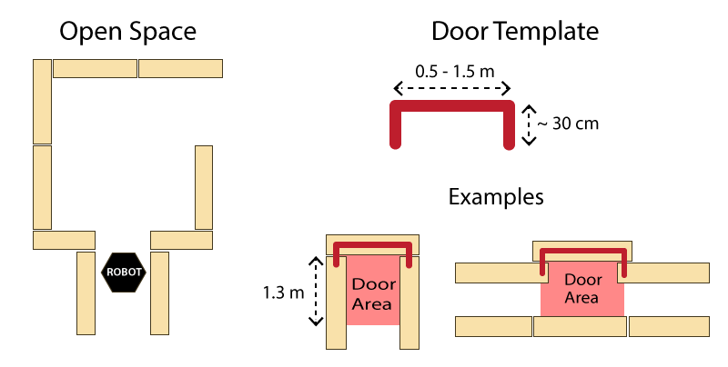
Doors and open spaces are specified as described by Figure 1.
Functions
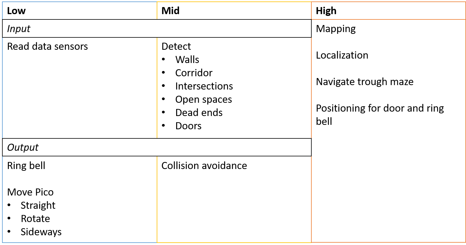
The functions are categorized in three different levels of complexity: Low, Mid and High level. An overview of the functions is given in Figure 2.
Components
The following components are accessible on the pico:
- Sensors
- Laser Range Finder (LFR)
- Wheel encoders (odometry)
- Actuators
- Holonomic Base (Omni-wheels)
- Computer
- CPU Intel i7
- OS Ubuntu 14.04
Interface
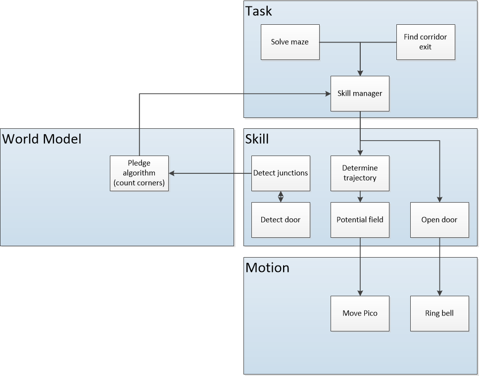
The interfaces between functions are shown in Figure 3. Here the functions are devided into: Tasks, Skills, Motions and the World Model. The world model contains the functions that are used to keep track of Pico's surrounding. Tasks contains the functions on the highest level where the robot decides what it is going to do, like solve the maze. The skill block consists of all functions that make the robot perform lower level tasks such that the high level objective can be achieved. The motion block does the low level operations that make the skill functions work.
The Corridor Challenge
Moving and cornering
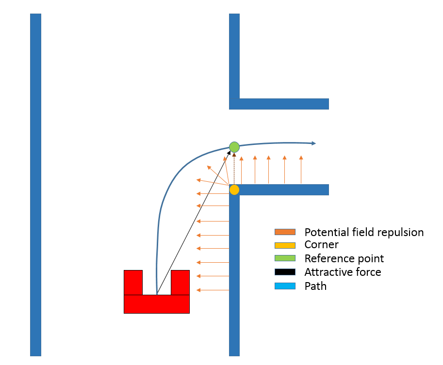
A couple of things are used in order for Pico to move through the corridor and make a corner. The first thing is a potential field. This creates an artificial bubble around Pico which repels it from objects that get too close. The second thing that allows Pico to make the corner in the corridor is its corner detection. This corner detection analyses the data from Pico's laser sensor and finds the corners of the corridor. When Pico approaches a corner on either side of the corridor, a reference point is placed beyond this corner in the middle of the hallway Pico should turn into. An attracting force is created that pulls Pico straight towards this reference point. Of course Pico can't go straight to this reference point since part of the wall is in the way and Pico is pushed from this by the potential field (see Figure 4). This combination of attraction and repulsion creates a curved path around the corner and into the exit of the corridor. Pico keeps cornering until either the odometry has detected that a turn of more than 1/2 Pi radians has been made or until the point around which Pico is cornering has been lost out of sight. As shown in the corridor challenge result video below, a drunk Pico makes a beautiful turn to exit the corridor. In the two following sections the inner workings of the potential field and the corner detection are explained in greater detail.
Potential field
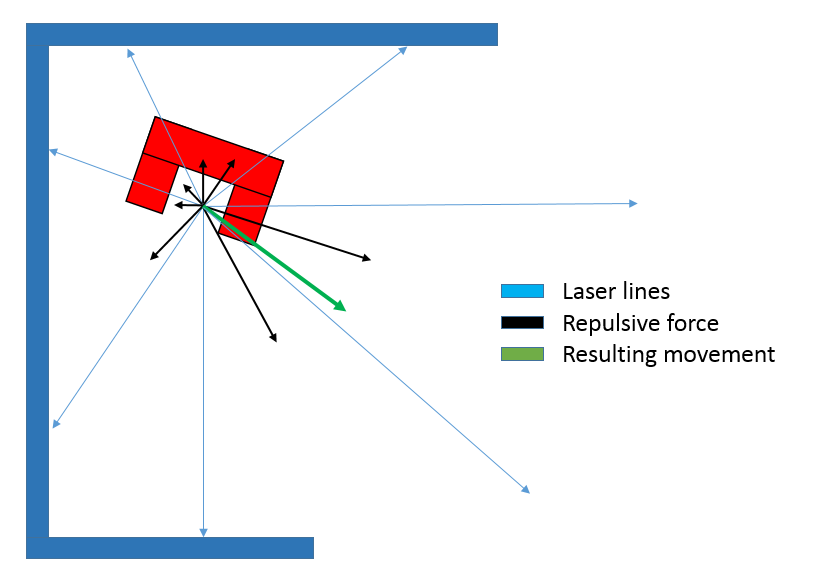
In order for Pico to safely manoeuvre through the corridor, a potential field is implemented. This potential field will push Pico away from walls with a force that gets bigger the closer Pico gets to a wall. The size and direction of this force is calculated based on the data gained from the laser sensor. First, the length of all 1000 laser lines is inverted and the angle of each line is shifted over an angle of Pi radians. This creates vectors that point away from obstacles with a force that increases the closer an obstacle is to Pico. After that, all converted vectors are split into x and y segments which are summed up and recombined to create a single vector pointing away from any obstacles. The size of the resulting vector equals the force, and thus speed, with which Pico is pushed away from the obstacles. In order to make the behaviour of Pico more predictable the size of the resulting vector is normalized and rescaled based on the closest object at a later point. Rescaling all vectors that influence Picos movements (potential field and reference point from previous section) based on the distance to the nearest object creates a clear overview of how these different forces interact and make Pico move. Figure 5 visualizes the potential field.
Corner detection
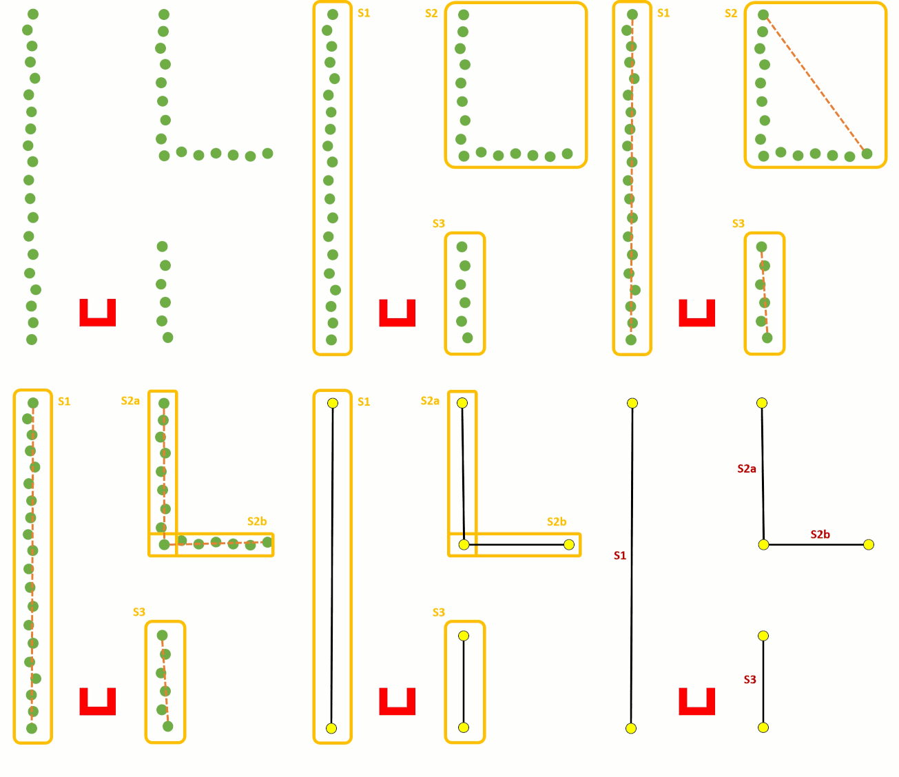
To detect corners and walls the 'Split and Merge' algorithm is used on the laser data. This algorithm contains the following procedure:
- 1. Laser data is transformed into x and y coordinates
- 2. Laser data points will grouped into segments
- 3. Within each segment a line is drawn between the first and last point and the perpendicular distance between each other point and this line is checked
- 4. If the maximum perpendicular distance is above a set threshold (0.2 m), this point will be set as a vertex within this segment.
- 5. Step 3 and 4 will be repeated until there are no new vertices are found.
- 6. Within each segment a line will be defined using the least squire method.
- 7. If two lines are connected with each other, the intersection will be used to define the vertex.
- 8. If there a line has no further connections, the last point of the line will be set as an end point.
These steps are visualized in the figure below:
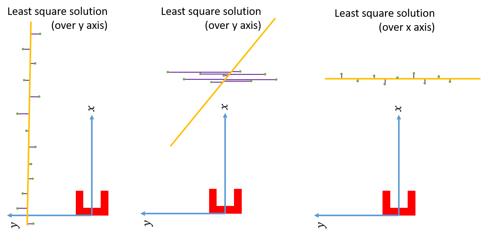
To create a better and more stable fit of lines on the data, the standard 'Split and merge' algorithm has been expanded with a 'Least Square Method'. As can be seen in the first situation in the figure below, there is a wall left of Pico. Using the standard Least Squire Method, a line (yellow) is constructed where the error (purple) between the points and the line is minimized over the y axis. However, if there is a wall in front of pico, as shown in the second situation, the least squire method finds a line that is not equal to the orientation of the wall. This is because the standard method minimizes the error over the y axis. If the same procedure method is used over the y axis, as shown in the third situation, the found line has the same orientation as the wall. Therefore, the Least Square Method is extended so that the Least Square Solution over x or y axis is picked for which one the error is the smallest.
Visualization corner detection
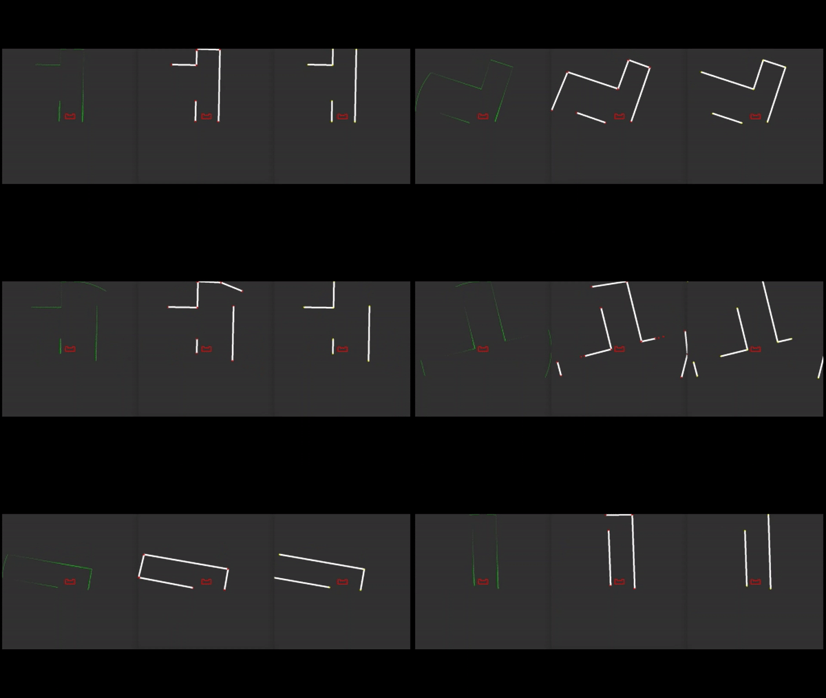
In order to test the corner detection, a visualization is made based on the existing code from 'emc-viz'. With this visualization it is easier to see what pico observes. On the left in green dots, the raw laser data is shown. In the middle the result after the split and merge algorithm is applied. On the right the walls and corners are shown after removing false walls and applying the Least Square Method. From this GIF it is visible that the error on the edges and lines is reduced, and the results are more stable/robust.
Challenge Result
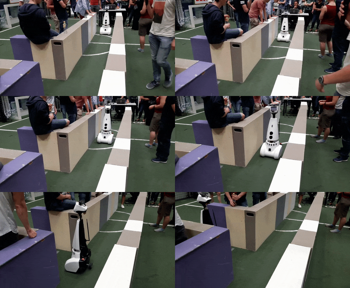
Pico managed to finish the corridor challenge in 24 seconds, this got us the third place. As can be seen in die video on the straight the Pico wobbles a lot this is due to the over reactive implementation of the potential field. Without this wobbling we would possible be in the first place due to the very smooth corner.
The Maze Challenge
Final design
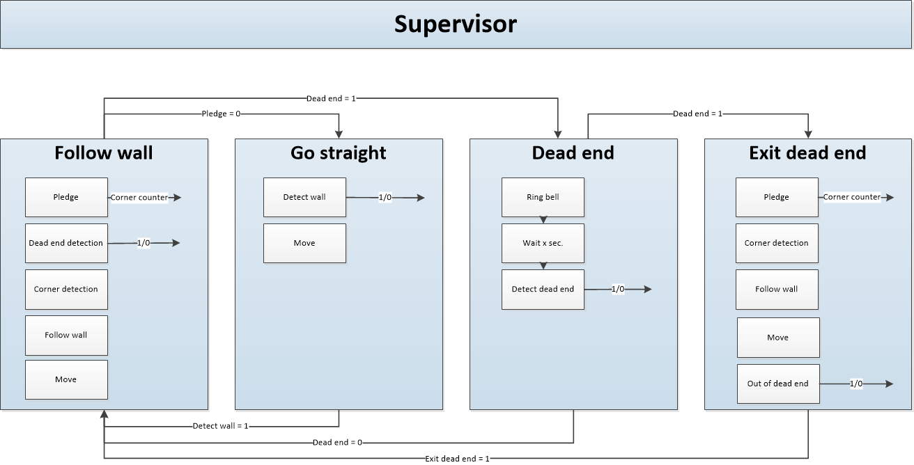
To solve the maze challenge there are designed individual parts, which will be explained in the next part. To manage these individual parts the state machine shown in Figure 7 is needed. This state machine switches from one state to another based on the given outputs. The start state of the state machine is 'Go Straight', this is because the counter of the Plegde algorithm start at zero and Pico should not follow a wall in these conditions. Pico stays withing this state until it detects a wall in front of it. To do this it uses the function 'Detect wall'. This function simply checks the range of the front facing laser beams. If the detected range gets below a threshold, the state machine switches to the 'Follow wall' state. In order to move the robot straight ahead, the 'Go straight' state also has a function to move the robot. In order to prevent deadlocks in certain situations the robot always returns to the 'Follow wall' state after leaving another state. Before doing anything in the 'Follow wall' state, conditions are checked for dead ends and the pledge algorithm is updated. If a dead end is found the robot will switch to the 'Dead end' state. If the pledge counter is set to zero and no dead end is detected, the robot will enter the 'Go straight' state.
Part of the maze challenge is to open a door which can be seen as a dead end because of the specifications of a door in the assignment. Attempting to open a door should therefor only be done when the robot finds itself near a dead end. Because of this, the 'Ring bell' functionality to open the door is located inside the 'Dead end' state. To get in the 'Dead end' state the 'Follow wall' state has a function called 'Dead end detection'. When this results in a positive outcome, the state machine switches to the 'Dead end' state. Once inside the 'Dead end' state the robot attempts to open the door by ringing a bell and waiting 5 seconds. This has two potential outcomes. Either the dead end had a door, or it didn't. The robot checks which outcome is the case by rerunning the 'Dead end detection' function. If it finds no dead end it means there was a door and it has been opened. The robot can now resume its wall following by returning to the 'Follow wall' state. If it still finds a dead end however, it means there was no door and the robot is simply located in a real dead end. To prevent a dead lock in which the robot keeps checking for dead ends and trying to open a door that isn't there, the robot enters the 'Exit dead end' state. In this state the robot will resume its normal wall following behavior, but without checking for dead ends. It will stay in this state until it has moved more than one meter away or turned more than 180 degrees from the position where it entered the state. When these conditions are met the robot will reenter the 'Follow wall' state.
With these four states and the individual functions, Pico should be capable of solving the maze challenge. The following sections will give in depth explanations of the functions that have not been explained before (Wall following, Pledge, Dead end detection).
Individual state machine functions
Wall following
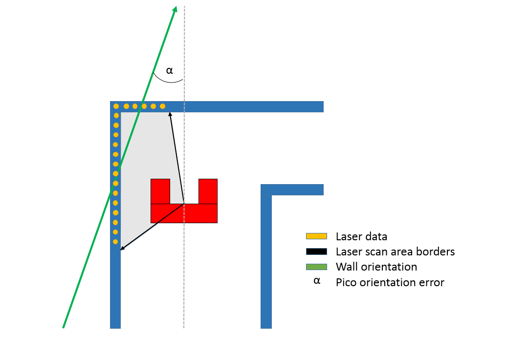
To implement the pledge based strategy it is necessary for Pico to be able to follow a wall in a robust manner. For this goal a wall following function has been implemented. This function makes use of some of the functionality of the corner detection explained earlier. This used part connects the individual laser dots and forms a single line that follows the overall direction of the wall (see Figure 8). Based on this line a reference point at a fixed distance from the wall is set for the robot. Using a PD-controller, the robot is then moved to keep itself at this reference point. Another PD-controller is used to keep the difference between the angle of the wall and Pico close to zero. This causes Pico to drive parallel to the wall. The two PD-controllers are then combined with the potential field to make sure Pico never bumps into any walls. Finally, to move Pico forward, a fixed reference point is placed in front of it which moves it forward at maximum speed when no obstacles are detected.
In order to balance the three different forces at work (PD-controllers, potential field, forward reference), each force is scaled based on the distance and position of to the closest object. When, for instance, no objects are detected in front of pico and pico is oriented perfectly parallel with the wall, the potential field and PD-controller for the angle are scaled down significantly and will influence Picos speed very little. However, when taking a corner along an outside wall, Pico will detect that the angle of the wall it is following deviates from its own. It will also detect the wall in front of it. These conditions will respectively increase the influence (gain) of the PD-controller for the angle and the potential field. Both will also decrease the influence of the forward reference, causing Pico to slow down and carefully make the corner.
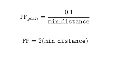
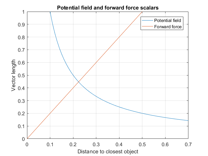
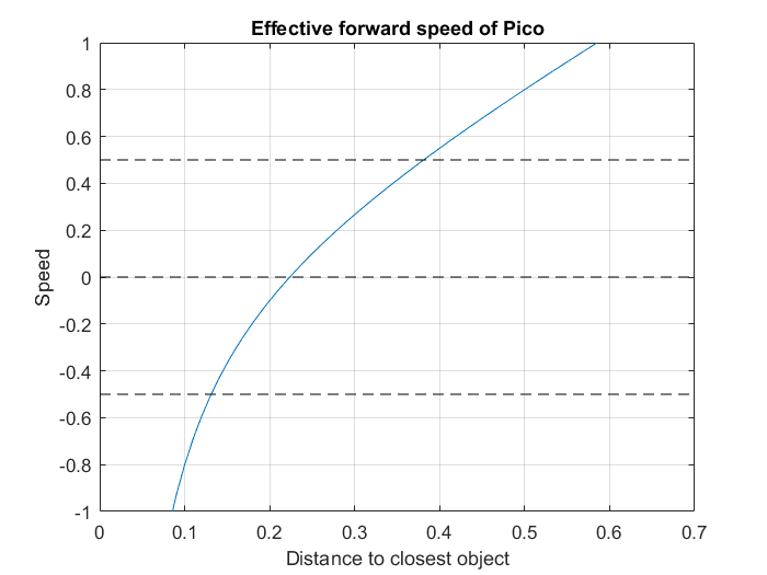
An example of balancing these forces to avoid collision is given in Figures 10 and 11. These plots show the scaling of the potential field and forward force based on the formulas given in Figure 9. Besides scaling the three earlier mentioned forces to make sure Pico drives smooth and fast along the walls, the following example acts like a final safety net to avoid any collision. Figure 10 shows the vector lengths of the potential field and the force of the forward reference based on the distance to the closest object detected by the laser. When Pico drives head on towards an object, the potential field works in exactly the opposite direction as the forward force. To calculate the effective speed in this situation the length of the potential field vector can be subtracted from the length of the forward force vector. Figure 11 shows the resulting speed of Pico when this is done. What shows is that Pico will drive at full speed when there is approximately 38 cm of free space in front of it. When objects get closer it quickly decelerates and stops when objects get as close as 22 cm. If objects get any closer, the potential field will become stronger than the forward force and Pico will drive backwards. The distance between the laser sensor and the front of Picos body is approximately 15 cm. This leaves 8 cm of extra room for Pico to stop and move backwards. Test have shown that this is sufficient room for Pico to avoid any collision. In the first Maze challenge try (video is shown further down), it can be seen that Pico stops perfectly in front of any wall and always avoids collisions.
Pledge
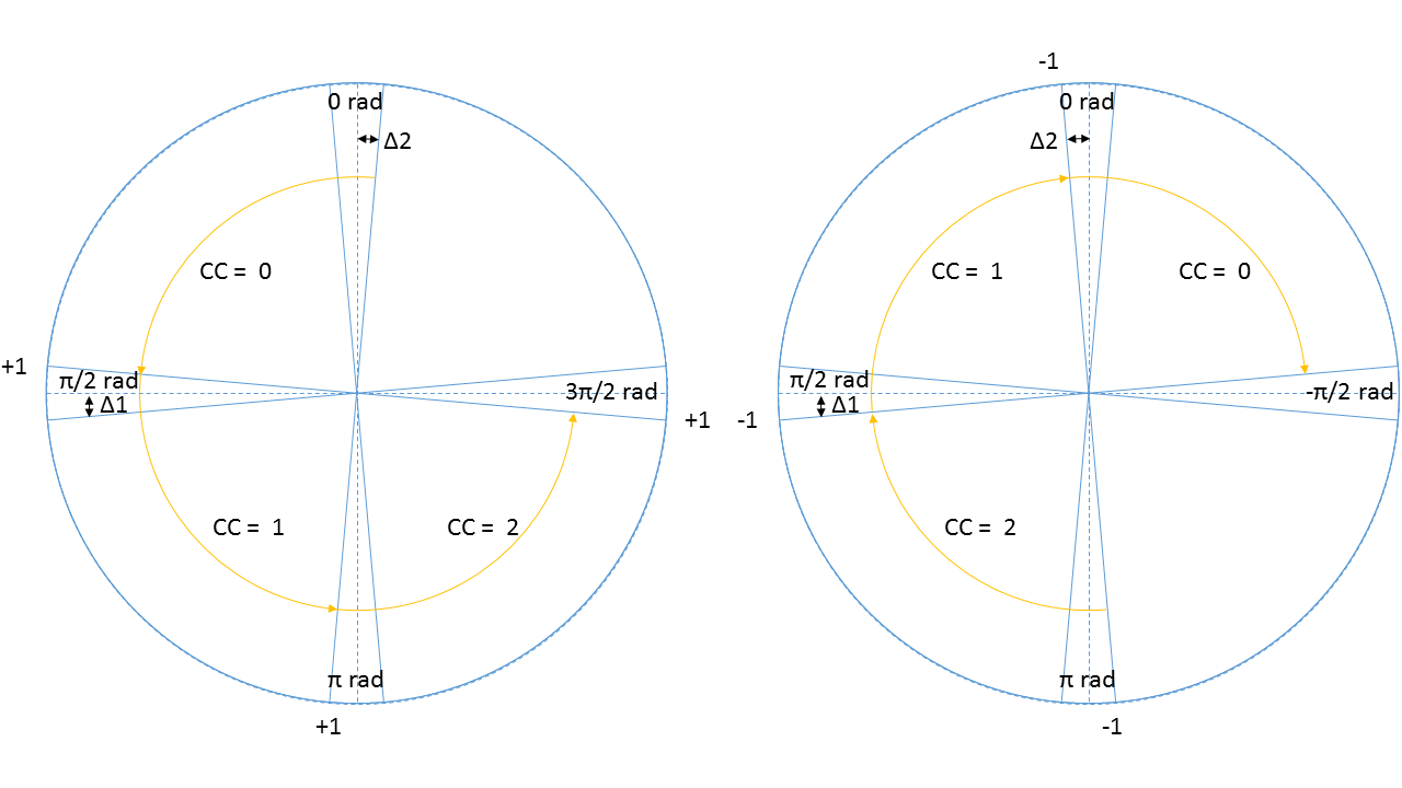
The Pledge algorithm is used to make a very simplistic global world map to solve the maze. The pledge algorithm uses relative angle movements to calculate the total rotation angle of the robot and keep track of the 'Pledge score'. A 90 degree turn to the left equals +1 for this 'Pledge score', a 90 degree turn to the right equals -1. When this score reaches zero, the state machine should switch to the 'Go straight' functions in order to find a new wall to follow. To make the pledge algorithm robust, a method is used where a corner is counted after the robot turns 1/2 Pi minus a small term (Delta 1 and 2 in Figure 12). In between these areas, the robot can move freely without the corner count being changed. Figure 12 shows two situations. The left circle shows the points (indicated with +1) at which the corner count goes up by one when making left turns. The right circle shows the points at which the corner count goes down by one when making right turns.
A problem arises when the corner count becomes zero and the robot switches to the 'Go straight' state. The moment the corner counter becomes zero, the robot will stop following the wall and drive straight ahead. To increase robustness the area at which a corner is counted is increased with a term Delta 1. However, this has the downside that the corner counter will be set to 0 just a bit before the robot completed its 90 degree turn. The robot will now drive straight ahead while not being parallel to the wall (this is also visible in the first try of the maze challenge). To decrease the amount the robot deviates from the wall, a second smaller delta term is used when the counter gets close to 0.
Another problem arises when the robot turns beyond a certain point. At this point the angle that is measured by the odometry switches from Pi to -Pi. This results in a relative angle of 2 Pi, which will wrongly increase or decrease the corner counter. To compensate for this, a check is done to see if the measured relative angle between two measurements is within set thresholds. When it is not, 2 Pi is subtracted from the measured relative angle which leaves only the relative angle which the robot actually turned.
Dead end detection
The dead end detection method makes use of the corner detection method as used in the corridor challenge.
The corner mapping returns the vertices's of the line segments it has found, and if the vertices's are connected to each other. This information is used by the corner detection to form vectors between these vertices's.
These vectors are then normalized so they can be used to determine the angle between them. If two vectors are connected, the angle is calculated using the following function

Where [math]\displaystyle{ \theta }[/math] is the angle between the vectors and vi • vi+1 is the inner product of vector i with i+1. If this angle is 90±5 degrees, the corner is marked perpendicular. The calculated angle does not give information on the sign. A vector pointing to the left or right result in the same angle (as the inner product between almost perpendicular vectors is approximately 0). In order to determine the direction of the turn, the vector vi is rotated 90 degrees to the left, using a rotation matrix. The inner product is then calculated again, if the result is positive, then the turn is to the left. If rotating the vector to the right results in a positive inner product, then the turn is to the right. All vectors are checked in this fashion, resulting in a list of left-, right- or no-turns, describing all corners visible to the robot.
Using the list of turns, possible dead ends can be identified. An important aspect of the list of vertices's is that it is generated in an anti clockwise direction. Therefore it is known that when two left turns follow after each other indicate a dead end candidate. Since the walls of the dead end candidate can be long, and therefore can just be a wall in the maze, further identification is done. The specifications of a dead end are given in the specifications above. There it is noted that the width of the dead end has to be within (0.5 < width < 1.5) [m]. So when a possible dead end is found, the width of that dead end candidate is checked. If it fails, the dead end is dropped. If it passes the minimum depth of 0.3 [m] is checked. If that also passes the dead end will be marked.
As all turns in the turn vector have been evaluated, the dead end closest to pico is returned from the dead end detection method for furher use in the state machine.
Matrix multiplication, matrix norms and inner products where used in this function to make the implementation easier. Here fore the Eigen library was used, this made working with matrices a lot more convenient (almost matlab like). The implementation of the function is found on git dead end detection
Final challenge result
After the mild succes at the corridor challenge, a complete overhaul of the approach to the problem was done. For the corridor challenge the robot relied too much on its potential field. This resulted in drunk movements from one wall to the other. To change this the potential field was given a backseat, only functioning as a final safety net. For the primary motion skill the 'follow wall' function was created. This makes use of laser data to find the distance from and direction of the nearest wall. Using two PD-controllers Pico is then positioned parallel to the wall and allowed to run at full speed if there are no obstacles in front of it. This robust and fast way of maneuvering through the maze and the robust implementation of the pledge algorithm resulted in a system that could easily solve any standard maze that was thrown at it. The maze for the challenge however, had a door.
In order to open the door it first needed to be detected. It was given in the assignment that the door was located in a dead end. Reusing the code that was able to convert laser data into vectors that form sections of walls that can be checked for the conditions of a dead end. Once a dead end is detected the bell can be ringed to attempt to open a door.
When we first tested the completed version of this maze solving program, the day before the challenge, we where amazed by the robustness of our code. All scenarios made up by us were solved without any effort. Walls where followed, loops in the maze were avoided, dead ends where found and doors were opened. All good. During the challenge itself however, a tiny little bug would wreck havoc upon our beautiful Pico.
The day of the challenge
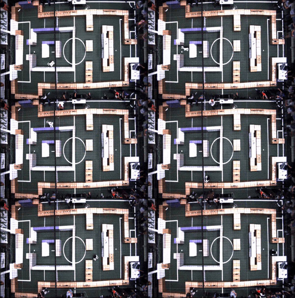
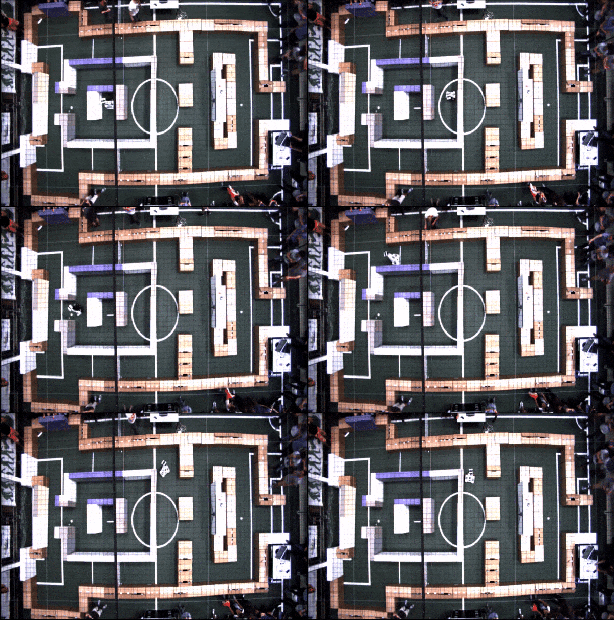
We were the last group to have a go at the challenge, the time to beat: 2:43 minutes. During the first attempt, great progress was made by Pico. The commentator was amazed by the speed of the little robot. Within no time, the door was found and opened. The only task left was finding the exit. It was looking very good. With about a 40 second lead people start to cheer as Pico begins his last turn towards to exit. This is where the tiny little bug from before decided to show up. With the finish line in sight, the program throws a segmentation error. With the finish line only 20 cm away, Pico comes to a sudden stop.
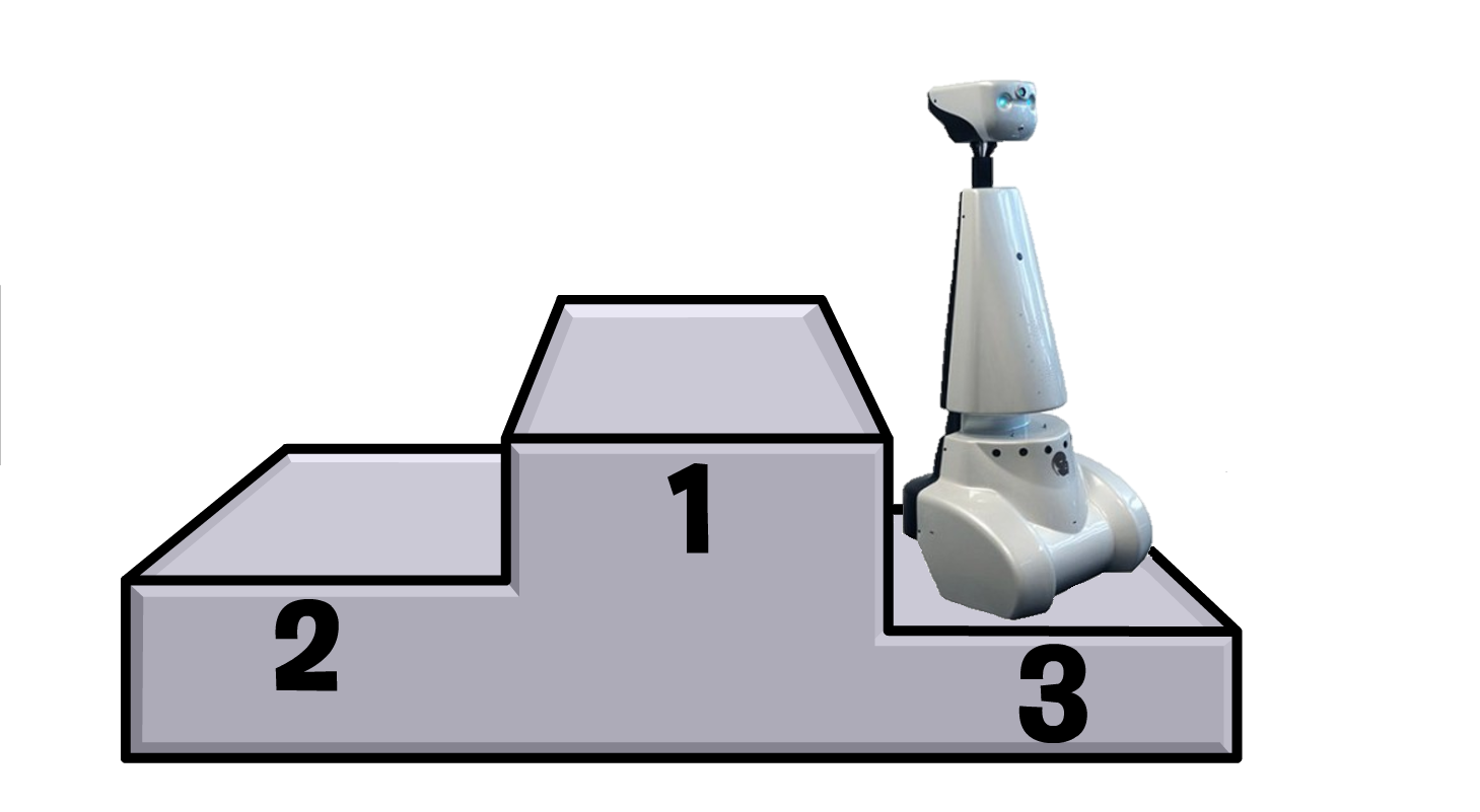
No worries we thought, we have had segmentation faults before. Sometimes they would just pop up in weird situations. We thought we had removed all warnings that had caused the segmentation errors before and thus found it strange that one would show up here, 20 cm in front of the finish line, but we just put it off as bad luck and started our second attempt. Knowing we were by far the fastest and hoping that the error was just a case of weird coincidence, we had good hopes for our seconds try. Pico was as fast and steady as during the first try. It managed to find and open the door again in no time. However, after taking another corner an error was thrown again and Pico stopped once more. Another segmentation error? No, this time the program crashed by a matrix multiplication error. This ends our second try resulting in a 3rd place. At the bottom of this section a video of both attempts can be viewed.
It is unclear to us where the matrix multiplication error came from. Even after testing many different situations we have never encountered this error nor were we able to reproduce it. The segmentation fault however was, unfortunately, a very easy fix. The error was caused by the robot detecting too many different elements in the net that was hanging near the exit of the maze. All these elements are stored in a matrix with a statically defined size. The matrix was too small to store all these elements, which resulted in a segmentation error. After the challenge, the size of the matrix was increased and the program was tested again. This time it worked fine.
A hard lesson was learned.
 |
 |
Evaluation
We are very proud of the end result. Even though we technically did not finish the maze, we were the fastest ones to 'finish' the maze (up to the last corner). The movements of Pico were almost perfect. When closing in on a wall he slowed down and turned without colliding with anything. When moving along a wall and no obstacles were in the forward direction Pico went full speed ahead, just like a real robot should. The dead end detection also worked flawlessly. Not a single wrong measurement was done for the dead end detection. The pledge algorithm also worked very well and guided the robot flawlessly out of the loops that were present in the maze. All of this could not have worked without a very robust method to detect the walls and corners around Pico. So it goes to say that the corner detection worked marvellous as well. Overall we are again very pleased with the result.
Of course there were also many things that went wrong during the design and implementation of the program. To sum up some important lessons we have learned from this course. It is important to really think something through before starting the implementation. Sometimes sitting down that one extra time to think everything through and question your ideas leads to new insights. For us, this resulted in giving the potential field a back seat and guiding the robot along the maze by following the walls. Letting it move at high speed towards open space instead of letting it pay too much attention to unimportant objects that might be close by, but are in no way in its path. It is also very important to clearly work out your ideas on paper before starting to implement them. This would have saved us a lot of tweaking, fixing and redoing little things. The harshest lesson of all is to always create matrices and other parts of your code to which you write data to have a size that can be dynamically adjusted. This will prevent segmentation faults by not accidentally writing to memory that cannot be accessed. If nothing else, at least use try() and catch() structures to catch any unforeseen exceptions.
Code Snippets
These are some of the code snippets of which we are especially proud. The first snippet shows the config file we use to configure the behaviour of Pico. All settings necessary to tune or debug Pico can be set from here. We are especially proud of the typedefs at the bottom of this file, which are used in for instance the environment scan function. Since we didn't want to struggle with creating lists of pointers to use as matrices, we defined these typedefs to use as objects that can be initialized where needed, and store all the necessary information they were created for.
The second code snippet shows the 'Dead end detection' used during the maze challenge. We are proud of this code snippet since it uses the template matching taught during the lectures. In the code a template for what a dead end should look like is defined. The incoming laser data is mapped on this template to see if there is a match.
The third code snippet shows the least square method from the corner detection. We are proud of this code snippet because of its simplicity, clearness and robustness.