Viotar/Quantifying the signal: Difference between revisions
No edit summary |
|||
| (24 intermediate revisions by 3 users not shown) | |||
| Line 1: | Line 1: | ||
{|cellpadding="10" | {|cellpadding="10" | ||
|-valign="top" | |-valign="top" | ||
|width="100%" style="border:1px solid #fabd23; background-color:#FEF5DE;"| | |width="100%" style="border:1px solid #fabd23; background-color:#FEF5DE;text-align: justify;"| | ||
{| padding="0" cellspacing="0" style="margin-top:.2em; width:100%; background:none" | {| padding="0" cellspacing="0" style="margin-top:.2em; width:100%; background:none" | ||
| rowspan="32" width="5px" | | | rowspan="32" width="5px" | | ||
| rowspan="2" class="BGorange1" valign="middle" style="text-align:center; padding:.6em 10px .6em 10px; background-color:#A9D0F5; border-top:2px solid #2E9AFE; border-bottom:2px solid #2E9AFE" | | | rowspan="2" class="BGorange1" valign="middle" style="text-align:center; padding:.6em 10px .6em 10px; background-color:#A9D0F5; border-top:2px solid #2E9AFE; border-bottom:2px solid #2E9AFE" | | ||
<h1 style="font-size:180%; border:none; margin:0; padding:0"> | <h1 style="font-size:180%; border:none; margin:0; padding:0"> | ||
'''Quantifying the signal | '''Software design - Quantifying the signal | ||
''' | ''' | ||
</h1> | </h1> | ||
| Line 24: | Line 24: | ||
'''Subpages:''' | '''Subpages:''' | ||
</h1><br/> | </h1><br/> | ||
{{:Viotar_Menu}} | |||
|width="2%" style="background-color:#FEF5DE;"| | |width="2%" style="background-color:#FEF5DE;"| | ||
|width="49%" style="border:2px solid #fabd23;"| | |width="49%" style="border:2px solid #fabd23;text-align: justify;"| | ||
<h1 style="font-size:180%; border:none; margin:0; padding:0"> | <h1 style="font-size:180%; border:none; margin:0; padding:0"> | ||
'''Overview:''' | '''Overview:''' | ||
| Line 50: | Line 36: | ||
|}<br/> | |}<br/> | ||
{| cellpadding="10" | |||
|-valign="top" | |||
| style="border:2px solid #00FF33; background-color:#CCFF99"| | |||
==Software Design (Quantifying the signal we want to see)== | ==Software Design (Quantifying the signal we want to see)== | ||
With software design, we mean the way the controller is structured. There are many possibilities, but it is important to design the controller in such a way that it matches the requirements that are stated. The controller will be tested on a fixed point model of the string, so it is also important to verify that the model is accurate enough to represent the real string. Besides that, also the following questions need to be answered to come to a good software design: | With software design, we mean the way the controller is structured. There are many possibilities, but it is important to design the controller in such a way that it matches the requirements that are stated. The controller will be tested on a fixed point model of the string, so it is also important to verify that the model is accurate enough to represent the real string. Besides that, also the following questions need to be answered to come to a good software design: | ||
| Line 108: | Line 96: | ||
These are 4 equations with 6 unknowns, so the system can't be solved. Therefore, the measurements of the 1st and 13th frets are dropped, because they are now only excess measurements. | These are 4 equations with 6 unknowns, so the system can't be solved. Therefore, the measurements of the 1st and 13th frets are dropped, because they are now only excess measurements. | ||
===Possible controller architectures=== | ===Controller Design=== | ||
====Possible controller architectures==== | |||
Before we can decide what type of controller would be best for our system, let's take a look at the possible controller architecture. The first type of controller is open loop (feed forward). This means that the controller only sends a signal to actuators without checking whether the desired requirements are achieved or not. The second architecture is a closed loop (feedback) controller. This controller compares a measured value with a pre-defined value and | Before we can decide what type of controller would be best for our system, let's take a look at the possible controller architecture. The first type of controller is open loop (feed forward). This means that the controller only sends a signal to actuators without checking whether the desired requirements are achieved or not. The second architecture is a closed loop (feedback) controller. This controller compares a measured value with a pre-defined value and adapts the system, untill the measured value equals the pre-defined value. At last, there is a combination of both. In this controller, all the known information is used to send a feed forward signal to bring the system as close as possible to the desired state. The small changes are made using the feedback signal. This controller is generally preferred above the feedback only controller because controlling on the feedback signal is mostly rather slow. | ||
Reflected on our viotar, this gives the following concepts: | Reflected on our viotar, this gives the following concepts: | ||
| Line 123: | Line 112: | ||
First, the right bow force and speed are determined using the lookup table, and actuated. Then, the comparison with the ideal Helmholtz signal starts, creating a feedback loop using this “tone quality”. This feedback signal is only used for fine-tuning the bow force and speed. | First, the right bow force and speed are determined using the lookup table, and actuated. Then, the comparison with the ideal Helmholtz signal starts, creating a feedback loop using this “tone quality”. This feedback signal is only used for fine-tuning the bow force and speed. | ||
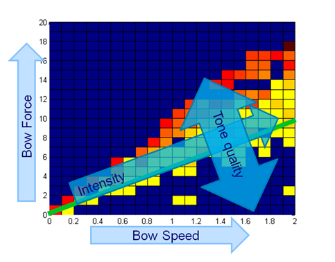
A combination of feed forward and feedback theoretically leads to the best result. That's why we choose to work this concept out first. In theory this means that tone intensity and quality will be controlled in the way shown in figure 6. | A combination of feed forward and feedback theoretically leads to the best result. That's why we choose to work this concept out first. In theory this means that tone intensity and quality will be controlled in the way shown in figure 6. In order to do that, we need to be able to recognize Helmholtz and quantify the signal. This can be done in both time and frequency domain as we will see later. | ||
[[File:controller_int_quant.PNG|frame|Border|center|Figure 6: Quality and intensity paths]] | [[File:controller_int_quant.PNG|frame|Border|center|Figure 6: Quality and intensity paths]] | ||
====Recognising Helmholtz and quantifying the signal==== | ====Recognising Helmholtz and quantifying the signal==== | ||
Probably, Helmholtz is the only harmonic vibration that you can get from a string when you bow it. With a bow you can never get a normal standing wave as when you would pluck the string. Because of this, it is not necessary to quantify "how much" the measured vibration is the specific Helmholtz waveform. It may suffit to merely quantify how harmonic the measured vibration is. This can be done by detecting the fundamental frequency in the Fourier transformation of the signal, and looking how many multiplications of this frequency are still in the signal. The more overtones, the sharper the Helmholtz, and therefore the better the tone. | |||
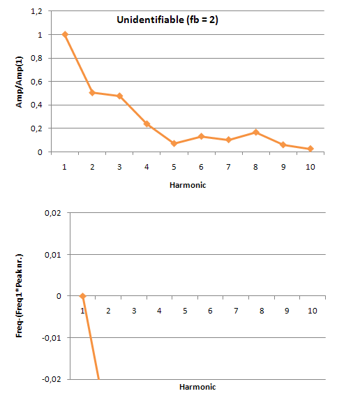
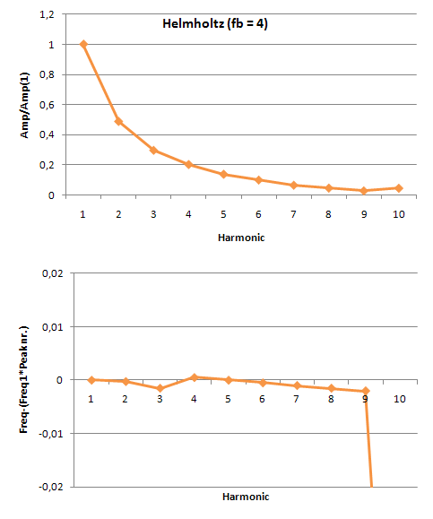
In order to do this we made amplitude plots in the frequency domain. This gives | In order to do this we made amplitude plots in the frequency domain. This gives information about the frequencies at which high peaks appear and what their amplitudes are. We did this for the model as well as for our measurements. When we first analyzed the model, we seemed to be right in the fact that as the tone gets better, more peaks appear in the power spectrum. These peaks are not randomly spread out, but appear at harmonic frequencies. That is, at n-times the fundamental frequency with n being the number of the peak. This is also made visible in the figures below. These figures show the difference between the frequency that you would expect following this rule and the actual frequency that comes out of the model. For an unidentifiable tone, there are no harmonic tones on the expected frequencies, as the graph runs out of the figure. For a clear Helmholtz vibration however, the rule is satisfied for nine peaks. A second thing that becomes clear by analyzing the results from the model, is that the amplitude of every next peak decreases exponentially. | ||
[[File:Model_unidentifiable.PNG|frame|Border|left|Figure | [[File:Model_unidentifiable.PNG|frame|Border|left|Figure 7: Amplitude ratio and frequency errors for an unidentifiable sound]] [[File:Model_helmholtz.PNG|frame|Border|center|Figure 8: Amplitude ratio and frequency errors for a Helmholtz vibration]] | ||
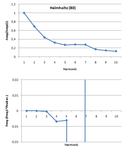
When we take a look at the measurements results, it becomes clear that these measurements are not as “clean” as the model. The same figures as for the model are also made for the measurements, as you can see below. The amplitude of the peaks does indeed decrease more or less exponentially as we would expect from the model. The number of peaks that appear at the expected frequency however, is only three for a vibration that sounded like a clear Helmholtz vibration to us. This can be explained by the fact that these measurements are done using a piezo element and the string vibrates along this element instead of perpendicular to it, which gives another signal. This problem is going to be solved however, because in the meantime experiments have proofed that the signal gets better when the string vibrates perpendicular, like it will on our prototype. | |||
[[File:Metingen_helmholtz.PNG|frame|Border|center|Figure 9: Amplitude ratio and frequency errors for measured Helmholtz sound]] | |||
So, we seemed to be right in the fact that a vibration being Helmholtz has something to do with the frequencies at which harmonic peaks appear and the amplitude of that peaks compared to that of the fundamental frequency. There is only one important thing that makes this method of quantifying the signal irrelevant for our prototype control system. The point is that for this method a Fourier transformation needs to be done in the control unit in order to detect what the quality of the signal is. The problem is, that a Fourier transformation cannot be done instantaneously but only when enough information about the vibration is gathered. A simple rule tells that the resolution of the transformation equals 1/(sample time). In our case, where quality of the sound depends strongly on the exact frequencies where peaks appear, we should have a resolution in the frequency domain of at least 1 Hz. This means that the sample time for every transformation needs to be about a second, while the vibration needs to be adapted in several milliseconds up to several hundreds of seconds at most. So, this method is simply never going to satisfy our requirements. | |||
However, there is another way to perform this method, being in the time domain. When we take a look at the sawtooth like waveform of a Helmholtz vibration, we can already in the time domain draw some conclusions regarding to the quality of the vibration. The reason for this is that the harmonic peaks in the time domain, with their decreasing amplitudes, and the saw-toothed waveform in the time domain are strongly related to each other. A saw-toothed waveform essentially is a set of harmonic sinuses with decreasing amplitudes, being sharper when more harmonic sinuses are present. Putting this in an equation leads to the following expression for the signal, consisting of n harmonics: | |||
<math>f=\sum_{i=1}^{n}(1/n) sin(nt)</math> | |||
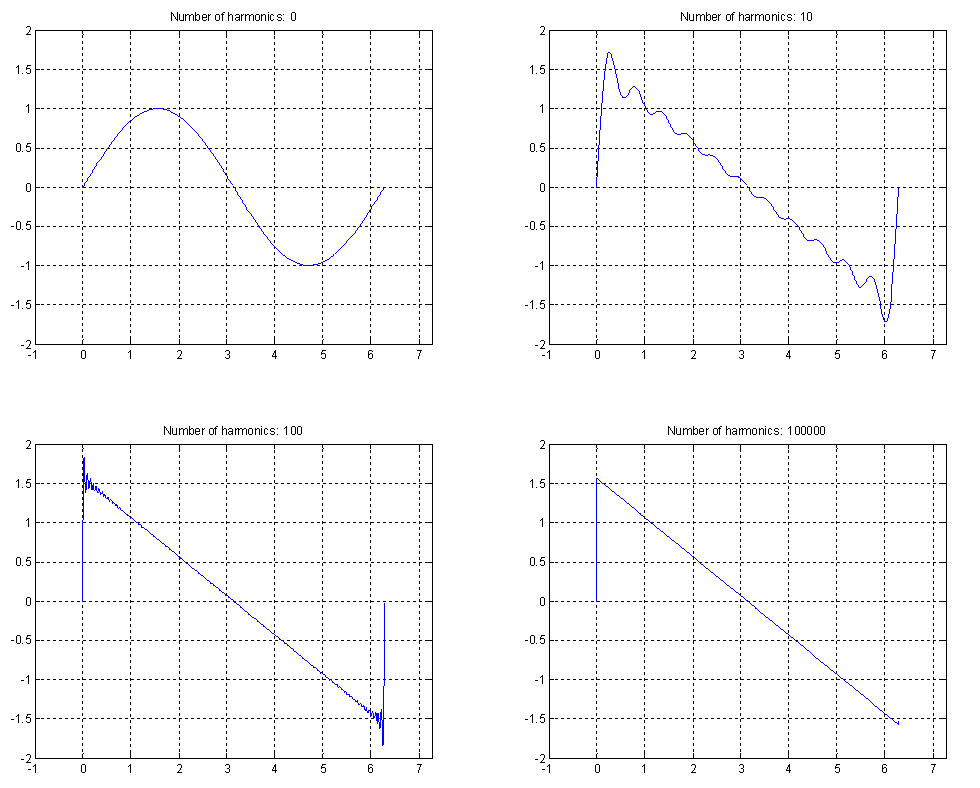
So the fact that more harmonic peaks appear in the frequency domain, finds is origin in the fact that more harmonic sinuses occur in the time domain. Moreover, when we want to quantify the signal in the time domain on the same properties as we did in the frequency domain, we only have to assess the signal on its sharpness. To proof this theory, figure 10 shows how the shape of the signal changes as the number of harmonic sinuses is increased. This leads to a perfectly sharp saw tooth, when the number of harmonic sinuses goes to infinity. | |||
[[File: Sawtooth_x4.PNG|frame|Border|center|Figure 10: Sawtooth signals for an increasing number of harmonics]] | |||
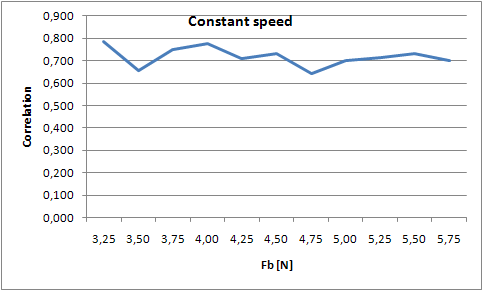
So, the idea is that we quantify the signal on the sharpness of the sawtooth. In order to do this we adapted our model and added a possibility to generate a sawtooth that serves as a reference. The correlation between the signal and our auto-generated reference sawtooth will be used as the quantification. This method will reduce the sample time to the longest period in the signal, which is 1 devided by the lowest frequency present in the signal. In this case the lowest frequency is about 100 Hz, so the sample time is about 10 milliseconds. To find out whether the signal indeed can be quantified on its sharpness (and thuss number of harmonics), we did some experiments. In the Helmholtz region, we varied the bowing speed at a constant bowing force and varied the bowing force at a constant speed. For all these simulations the correlation is calculated and plotted in the figures below (figures 11 and 12). From these figures, it can easily be concluded that there is not an ideal combination of bowing speed and force. That is, there is not an optimum which gives the best Helmholtz vibration. This means that when the vibration is a so called Helmholtz vibration, the system cannot be controlled to a point at which the correlation is highest. That is why we choose to make a lookup table with combinations of bowing speeds and forces that are in the Helmholtz region. The control unit then only needs to identify the fundamental frequency and lookup the right settings for the bowing speed and force. This gives great advantages regarding to adaptation time, because the controlling time now reduces to one sample time. | |||
[[File:Constant_force.PNG|frame|Border|left|Figure 11: Correlation for varying bowing speeds]] [[File:Constant_speed.PNG|frame|Border|center|Figure 12: Correlation for varying bowing forces]] | |||
====Controller concept==== | |||
The process described above, brought us to a controller design for the prototype. This controller makes use of a look-up table. This look-up table contains all the pre-defined values for bowing speed and force. By determining the fundamental frequency of the signal, the controller "knows" which fret is played and therefor what values for bowing speed and force are required. To make sure that the bowing speed indeed equals the value from the look-up table (also under varying bowing force) the engine speed is measured using an encoder and looped back to the controller. For the bowing force this does not seem to be neccesary, since the bowing force does not depend on the bowing speed. | |||
Latest revision as of 14:58, 23 March 2011
|

