Implementation MSD16: Difference between revisions
| (139 intermediate revisions by 4 users not shown) | |||
| Line 6: | Line 6: | ||
= Tasks = | = Tasks = | ||
The tasks which are implemented are: | |||
* Detect Ball Out Of Bound (BOOP) | |||
* Detect Collision | |||
The skill that are needed to achieve these tasks are explained in the section ''Skills''. | |||
= Skills = | = Skills = | ||
== Detection skills == | == Detection skills == | ||
For the B.O.O.P. detection, it is necessary to know where the ball is and where the outer field lines are. To detect a collision the system needs to be able to detect players. Since we decided to use agents with cameras in the system, detecting balls, lines, and players requires some image-processing. The TURTLE already has good image processing software on its internal computer. This software is the product of years of development and has already been tested thoroughly, which is why we will not alter it and use it as is. Preferably we could use this software to also process the images from the drone. However, trying to understand years worth of code in order to make it useable for the drone camera (AI-ball) would take much more time than developing our own code. For this project, we decided to use Matlab's image processing toolbox to process the drone images. The images comming from the AI-ball are in the RGB color space. For detecting the field, the lines, objects and (yellow or orange) balls, it is more convenient to first transpose the image to the [https://en.wikipedia.org/wiki/YCbCr YCbCr] color space. | |||
=== | === Line Detection === | ||
The line detection is achieved using [http://nl.mathworks.com/help/images/hough-transform.html Hough transform] technique. | |||
Since the project is a continuation of the MSD 2015 generations [http://cstwiki.wtb.tue.nl/index.php?title=Robotic_Drone_Referee Robotic Drone Referee Project] ; the previously developed line detection algorithm is updated and used in this project. The detailed explanation of this algorithm can be found [http://cstwiki.wtb.tue.nl/index.php?title=Line_Detection here.] | |||
Some updates have been applied to this code, but the algorithm is not changed. The essential update is the separation of the line detection codes from all detection codes which is created by the previous generation and creating the new function as an isolated skill. | |||
=== Detect balls === | === Detect balls === | ||
The flow of the ball detection algorithm is shown in the next figure. First, the camera images are filtered on color. The balls that can be used can be red, orange or yellow; colors that are in the upper-left corner of the CbCr-plane. A binary image is created where the pixels which fall into this corner get a value of 1 and the rest get a value of 0. Next, to do some noise filtering, a dilation operation is performed on the binary image with a circular element with a radius of 10 pixels. Remaining holes inside the obtained blobs are filled. From the obtained image a blob recognition algorithm returns blobs with their properties, such as the blob center and major- and minor axis length. From this list with blobs and their properties, it is determined if it could be a ball. Blobs that are too big or too small are removed from the list. For the remaining possible balls in the list, a confidence is calculated. This confidence is based on the blob size and roundness: | |||
confidence = (minor Axis / major Axis) * (min(Rblob,Rball) / max(Rblob,Rball)) | |||
<center>[[File:ImageProc_ball.png|thumb|center|1250px|Flow of ball detection algorithm]]</center> | |||
=== Detect objects === | === Detect objects === | ||
The object (or player) detection works in a similar way as the ball detection. However, instead of doing the color filtering on the CbCr plane, it is done on the Y-axis only. Since the players are coated with a black fabric, their Y-value will be lower than the surroundings. Moreover, the range of detected blobs which could be players is larger for the object detection than it was for the ball detection. This is done because the players are not perfectly round like the ball is. If the player is seen from the top, they will appear different than when the are seen from an angle. A bigger range of accepting blobs ensures a lower chance on true negatives. The confidence is calculated in the same fashion as in the ball detection algorithm. | |||
<center>[[File:ImageProc_objects.png|thumb|center|1250px|Fig.1: Flowchart for path planning skill]]</center> | |||
== Refereeing == | == Refereeing == | ||
=== | === Ball Out of the Pitch Detection === | ||
Following the detection of the ball and the boundary lines, the ball out of the pitch detection algorithm is called. Similar to the line detection case, the algorithm developed by the previous generation is used essentially. The detailed explanation of this ball out of pitch detection algorithm is given [http://cstwiki.wtb.tue.nl/index.php?title=Refereeing_Out_of_Pitch here]. | |||
Although this algorithm provides some information about the ball condition, it is not able to handle to all use cases. At that point, an update and improvement to this algorithm added to handle the cases where the ball position is predicted via the particle filter. Although the ball is not detected by the camera, the position of the ball with respect to the field coordinate system can be known (at least predicted) and based on the ball coordinate information, in/out decision can be further improved. This part added to ball out of pitch refereeing skill function. However, this sometimes yields false positives and false negative results as well. A further improvement for refereeing is still necessary. | |||
=== Collision detection === | === Collision detection === | ||
For the collision-detection we can rely on two sources of information: the world model and the raw images. If we can keep track of the position and velocity of two or more players in the world model, we might be able to predict that they are colliding. Moreover, when we take the images of the playing field and we see in the image that there is no space between the blobs (players), we can assume that they are standing against each other. A combination of both these methods would be ideal. However, since the collision detection in the world model was not implemented, we will only discuss the image-based collision detection. This detection makes use of the list of blobs that is generated in the object detection algorithm. For each blob in this list, the length of the minor- and major axes are checked. The axes are compared to each other to determine the roundness of the object. Moreover, the axes are compared with the minimal expected radius of the player. If the following condition holds, a possible collision is detected: | |||
if ((major_axis / minor_axis) > 1.5) & (minor_axis >= 2 * minimal_object_radius) & (major_axis >= 4 * minimal_object_radius)) | |||
== Positioning skills == | |||
Position data of the each component are able to be gotten in diverse methods. In this project, the planar position (x-y-ψ) of the refereeing agents (it is only the drone) is achieved using an ultra bright led strip that is detected by the top camera. The ball position is obtained using image processing and further post-processing of image data. | |||
=== Locating of the Agents : Drone === | |||
The drone has 6 degree-of-freedom (DOF). The linear coordinates (x,y,z) and corresponding angular positions roll, pitch, yaw (φ,θ,ψ). | |||
Although the roll (φ) and pitch (θ) angles of the drone are important for the control of the drone itself, they are not important for the refereeing tasks. Because all the refereeing and image processing algorithms are developed based on an essential assumption: Drone angular positions are well stabilized such that roll (φ) and pitch (θ) values are zero. Therefore these 2 position information have not been taken into account. | |||
The top camera yields the planar position of the drone with respect to the field reference coordinate frame which includes x, y and yaw (ψ) information. However, to be able to handle refereeing tasks and image processing, the drone altitude should also be known. The drone has its own altimeter and the output data of the altimeter is accessible. The obtained drone altitude data is fused with the planar position data. The obtained information from the different position measurements are composed in the vector given below and this vector is used as ‘droneState’. | |||
Then the agent position vector can be obtained as: | |||
<math display="center">\begin{bmatrix} x \\ y \\ \psi \\ z \end{bmatrix}</math> | |||
== Locating | === Locating of the Objects : Ball & Player === | ||
As a result of the ball and object detection skills, the detected object coordinates are obtained as pixels. To define the location of the detected objects in the image, the obtained pixel coordinate should be transferred into the field reference coordinate axes. The coordinate system of the image on Matlab is given below. Note that, here, the unit of the obtained position data is pixels. | |||
[[File:FrameRef_seperat2.png|thumb|centre|400px|Fig.: Coordinate axis of the image frame]] | |||
Followingly, the pixel coordinates for the corresponding center of the detected object or ball, calculated according to the center of the image. This data is processed furtherly, regarding the following principles: | |||
* The center of the image is assumed to be focal center of the camera and this is coincident with the center of the image. | |||
* The camera is always parallel to the ground plane, neglecting the tilting of the drone on drone's roll (φ) and pitch (θ) axes. | |||
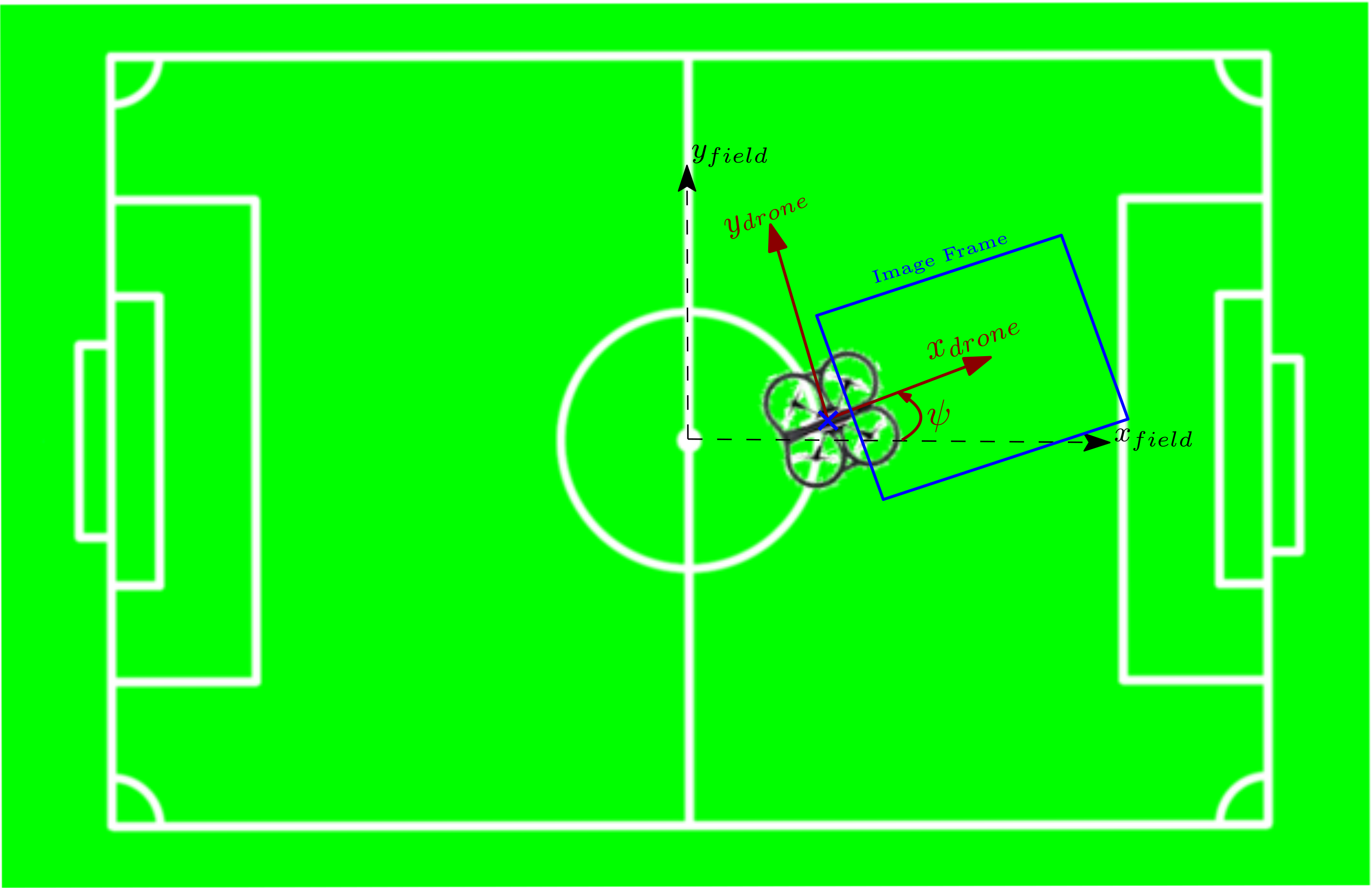
* The camera is aligned and fixed in a way that, the narrow edge of the image is parallel to the y-axis of the drone as shown in the figure below. | |||
* The distance from the center of the gravity of the drone (which is its origin) to the camera lies along the x-axis of the drone and known. | |||
* The height of the camera with respect to the drone base is zero. | |||
* The alignment between camera, drone and the field is shown in the figure below. | |||
[[File:RelativeCoordinates.png|thumb|centre|500px|Fig.: Relative coordinates of captured frame with respect to the reference frame]] | |||
Note that the position of the camera (center of image) with respect to the origin of the drone is known. It is a drone fixed position vector and lies along x-axis of the drone. Taking into account the principles above and adding the known (measured) drone position to the position vector of the camera (including the yaw (ψ) orientation of the drone); the position of the image center with respect to the field reference coordinate axes can be obtained. | |||
The orientation of the received image with respect to the field reference coordinate axes should be fitted according to the figure. | |||
Now, the calculated pixel units of the detected object, should be converted into real-world units (from pixels to millimeters). However this property changes according to the height of the camera. To achieve this, the height information of the drone should be used. Using the height of the drone and the FOV information of the camera, the ratio of the pixels to millimeters is calculated. More detailed information about FOV is given in the next sections. | |||
== Path planning == | == Path planning == | ||
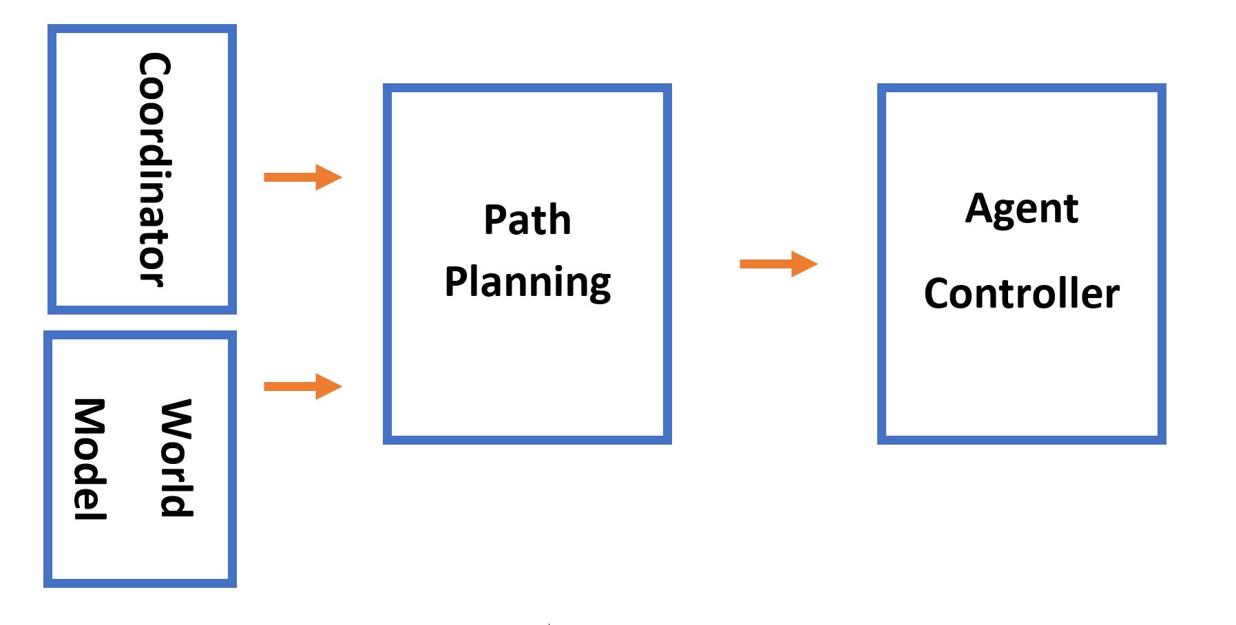
| Line 45: | Line 88: | ||
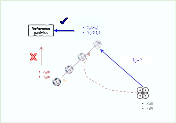
<center>[[File:pp-RefGenerator.jpg|thumb|center|750px|Fig.2:Trajectory of drone]]</center> | <center>[[File:pp-RefGenerator.jpg|thumb|center|750px|Fig.2: Trajectory of drone]]</center> | ||
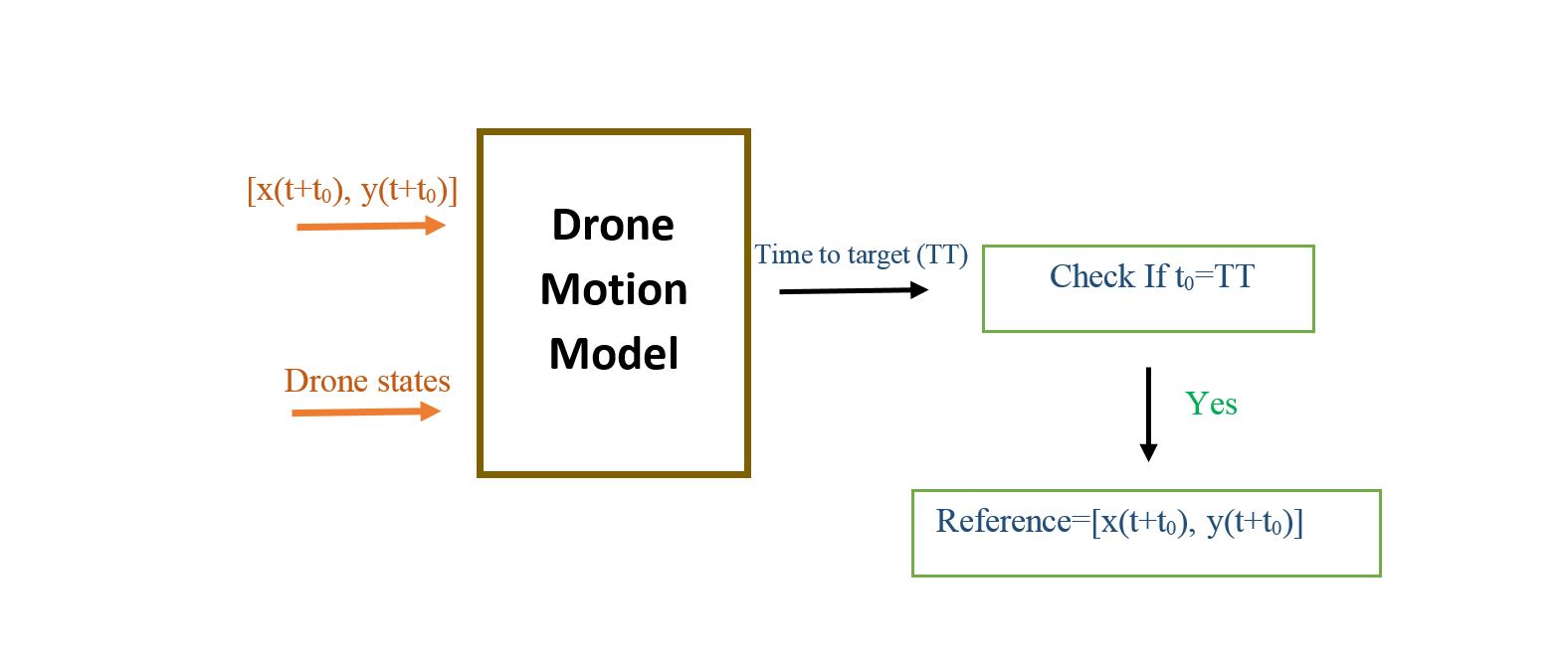
As it is shown in Fig.2, in a case of far distance between drone and ball, the drone should track the position ahead of the object to meet it in the intersection of the velocity vectors. Using the current ball position as a reference input would result in a curve trajectory (red line). However, if the estimated position of the ball in time ahead sent as a reference, the trajectory would be in a less curvy shape with less distance (blue line). This approach would result in better performance of tracking system, but more computational effort is needed. The problem that will be arises is the optimal time ahead t0 that should be set as a desired reference. To solve, we require a model of the drone motion with the controller to calculate the time it takes to reach a certain point given the initial condition of the drone. Then, in the searching Algorithm, for each time step ahead of the ball, the time to target (TT) for the drone will be calculated (see Fig.3). The target position is simply calculated based on the time ahead. The reference position is then the position that satisfies the equation t0=TT. Hence, the reference position would be [x(t+t0), y(t+t0)], instead of [x(t), y(t)]. It should be noted that, this approach wouldn’t be much effective in a case that the drone and object are close to each other. Furthermore, for the ground agents, that moves only in one direction, the same strategy could be applied. For the ground robot, the reference value should be determined only in moving direction of the turtle. Hence, only X component (turtle moving direction) of position and velocity of the interested object must be taken into account. | |||
<center>[[File:pp-searchAlg.jpg|thumb|center|750px|Fig.3: Searching algorithm for time ahead ]]</center> | |||
=== Collision avoidance === | |||
When Drones are flying above a field, the path planning should create a path for agents in a way that avoid collision between them. This can be done in collision avoidance block that has higher priority compared to optimal path planning that is calculated based on objective of drones (see Fig.4). Collision Avoidance-block is triggered when the drones state meet certain criteria that indicate imminent collision between them. Supervisory control then switch to the collision avoidance mode to repel the drones from getting closer. This is fulfilled by sending a relatively strong command to drones in a direction that maintain safe distance. Command as a velocity must be perpendicular to velocity vector of each drone. This is being sent to the LLC as a velocity command in the direction that results in collision avoidance and will be stopped after the drones are in safe positions. In this project, since we are dealing with only one drone, implementation of collision avoidance will not be conducted. However, it could be a possible area of interest to other to continue with this project. | |||
<center>[[File:pp-collisionAvoid.jpg|thumb|center|750px|Fig.4: Collision Avoidance Block Diagram]]</center> | |||
= World Model = | = World Model = | ||
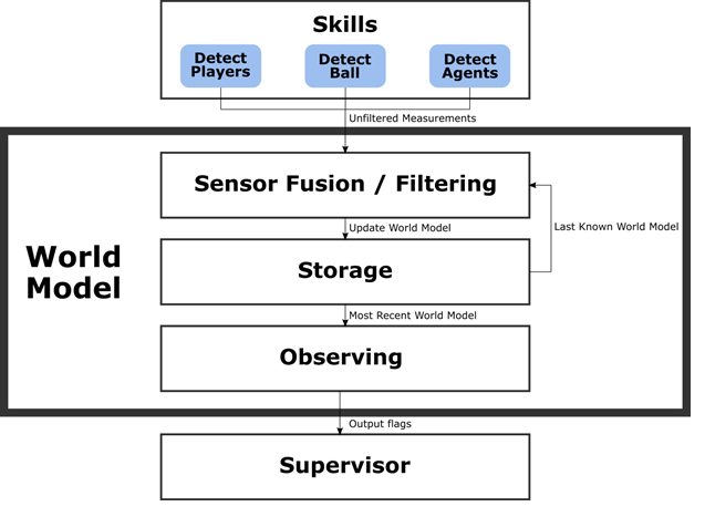
In order to perform tasks in an environment, robots need an internal interpretation of this environment. Since this environment is dynamic, sensor data needs to be processed and continuously incorporated into the so-called World Model (WM) of a robot application. Within the system architecture, the WM can be seen as the central block which receives input from the skills, processes these inputs in filters and applies sensor fusion if applicable, stores the filtered information, and monitors itself to obtain outputs (flags) going to the supervisor block. Figure 1 shows these WM processes and the position within the system. | |||
<center>[[File:worldmodel.png|thumb|center|750px|World Model and its processes]]</center> | |||
==Storage== | |||
One task of the WM is to act like a storage unit. It saves the last known positions of several objects (ball, drone, turtle and all players), to represent how the system perceives the environment at that point in time. This information can be accessed globally, but should only be changed by specific skills. The World Model class (not integrated) accomplishes this by requiring specific ‘set’ functions to be called to change the values inside the WM, as shown by Table 1. This prevents processes from accidentally overwriting WM data. | |||
<center>[[File:storage_table_1.png|thumb|center|750px|Set functions of the World Model ‘W’]]</center> | |||
Note that the WM is called ‘W’ here, i.e. initialized as W = WorldModel(n), where n represents the number of players per team. Since this number can vary (while the number of balls is hardcoded to 1), the players are a class of their own, while ball, drone and turtle are simply properties of class ‘WorldModel’. Accessing the player data is therefore slightly different from accessing the other data, as Table 2 shows. | |||
<center>[[File:storage_table_2.png|thumb|center|750px|Commands to request data from World Model ‘W’]]</center> | |||
==Ball position filter and sensor fusion== | |||
For the system it is useful to know where the ball is located within the field at all times. Since measurements of the ball position are inaccurate and irregular, as well as originating from multiple sources, a filter can offer some advantages. It is chosen to use a particle filter, also known as Monte Carlo Localization. The main reason is that a particle filter can handle multiple object tracking, which will prove useful when this filter is adapted for player detection, but also for multiple hypothesis ball tracking, as will be explained in this document. Ideally, this filter should perform three tasks:<br> | |||
1) Predict ball position based on previous measurement<br> | |||
2) Adequately deal with sudden change in direction<br> | |||
3) Filter out measurement noise<br><br> | |||
Especially tasks 2) and 3) are conflicting, since the filter cannot determine whether a measurement is “off-track” due to noise, or due to an actual change in direction (e.g. caused by a collision with a player). In contrast, tasks 1) and 3) are closely related in the sense that if measurement noise is filtered out, the prediction will be more accurate. These two relations mean that apparently tasks 1) and 2) are conflicting as well, and that a trade-off has to be made.<br><br> | |||
The main reason to know the (approximate) ball position at all times is that the supervisor and coordinator can function properly. For example, the ball moves out of the field of view (FOV) of the system, and the supervisor transitions to the ‘Search for ball’ state. The coordinator now needs to assign the appropriate skills to each agent, and knowing where the ball approximately is, makes this easier. This implies that task 1) is the most important one, although task 2) still has some significance (e.g. when the ball changes directions, and then after a few measurements the ball moves out of the FOV).<br><br> | |||
A solution to this conflict is to keep track of 2 hypotheses, which both represent a potential ball position. The first one is using a ‘strong’ filter, in the sense that it filters out measurements to a degree where the estimated ball hardly changes direction. The second one is using a ‘weak’ filter, in the sense that this estimate hardly filters out anything, in order to quickly detect a change in direction. The filter then keeps track whether these hypotheses are more than a certain distance (related to the typical measurement noise) apart, for more than a certain number of measurements (i.e. one outlier could indicate a false positive in the image processing, while multiple outliers in the same vicinity probably indicate a change in direction). When this occurs, the weak filter acts as the new initial position of the strong filter, with the new velocity corresponding to the change in direction.<br> | |||
This can be further expanded on by predicting collisions between the ball and another object (e.g. players), to also predict the moment in time where a change in direction will take place. This is also useful to know when an outlier measurement really is a false positive, since the ball cannot change direction on its own.<br><br> | |||
Currently, the weak filter is not implemented explicitly, but rather its hypothesis is updated purely by new measurements. In case two consecutive measurements are further than 0.5 meters removed from the estimation at that time, the last one acts as the new initial value for the strong filter. <br><br> | |||
When a new measurement arrives, the new particle velocity v_new is calculated according to<br><br> | |||
<center>[[File:equation_wm_particle.png|thumb|center|750px|]]</center> | |||
with v_old the previous particle velocity, z_new and z_old the new and previous measurements, X_old the previous position (x,y) and dt the time since the previous measurement.<br><br> | |||
The tunable parameters for the filter are given by table 1. Increasing α_v makes the filter ‘stronger’, increasing α_x makes the filter ‘weaker’ (i.e. trust the measurements more) and increasing α_z makes the filter ‘stronger’ with respect to the direction, but increases the average error of the prediction (i.e. the prediction might run parallel to the measurements).<br> | |||
<center>[[File:particle_filter_Parameters.png|thumb|center|750px|]]</center> | |||
As said before, measurements of the ball originate from multiple sources, i.e. the drone and the turtle. These measurement are both used by the same particle filter, as it does not matter from what source the measurement comes. Ideally, these sensors pass along a confidence parameter, like a variance in case of a normally distributed uncertainty. This variance determines how much the measurement is trusted, and makes a distinction between accurate and inaccurate sensors. In its current implementation, this variance is fixed, irrespective of the source, but the code is easily adaptable to integrate it.<br> | |||
==Player position filter and sensor fusion== | |||
In order to detect collisions, the system needs to know where the players are. More specifically, it needs to detect at least all but one players to be able to detect any collision between two players. In order to track them even when they are not in the current field of view, as well as to deal with multiple sensors, again a particle filter is used. This particle filter is similar to that for the ball position, with the distinction that it needs to deal with the case that the sensor(s) can detect multiple players. Thus, the system needs to somehow know which measurement corresponds to which player. This is handled by the ‘Match’ function, nested in the particle filter function. <br> | |||
In short, this ‘Match’ function matches the incoming set of measured positions to the players that are closest by. It performs a nearest neighbor search for each incoming position measurement, to match them to the last known positions of the players in the field. However, the implemented algorithm is not optimal in case this set of nearest neighbors does not correspond to a set of unique players (i.e. in case two measurements are both matched to the same player). In this case, the algorithm finds the second nearest neighbor for the second measured player. With a high update frequency and only two players, this generally is not a problem. However, in case of a larger number of players, which could regularly enter and leave the field of view of a particular sensor, this might decrease the performance of the refereeing system.<br> | |||
Sensor fusion is again handled the same way as with the ball position, i.e. any number of sensors can be the input for this filter, where they would again ideally also transfer a confidence parameter. Here, this confidence parameter is again fixed irrespective of the source of the measurement.<br> | |||
== Kalman filter == | == Kalman filter == | ||
The drone is actuated via UDP commend sent by host computer. The command contains the control signals in pitch angle, roll angle, yaw angle and vertical direction. The corresponding forward velocity and side velocity in bode frame can be measured by sensors inside the drone. At the same time, there are three LEDs on the drone which can be detected by camera on the top of the field. Based on the LEDs on the captured image, the position and orientation of drone on the field can calculated via image processing. <br><br> | |||
As the camera on the top of the field cannot detect the drone LEDs every time, kalman filter needs to be designed to predict the drone motion and minimize the measurement noise. Therefore, the further close loop control system for drone can be robust. As the flying height of drone does not have much requirement for system, the height part of drone is not considered in kalman filter design. | |||
<center>[[File:KF_Overview.png|thumb|center|750px|Command (a) is forward-back tilt -floating-point value in range [-1 1]. Command (b) is left- right tilt- floating -point value in range [-1 1]. d is drone angular speed in range [-1 1 ]. Forward and side velocity is displayed in body frame (orange). Position (x, y, Psi) is displayed in global frame (blue). ]]</center> | |||
=== System identification and dynamic modeling === | |||
The model needed to be identified is the drone block in figure 1. The drone block in figure 1 is regarded as a black box. To model the dynamic of this black box, predefined signals are given as inputs. The corresponding outputs are measured by both top cam and velocity inside the drone. The relation between inputs and outputs are analyzed and estimated in following chapters. | |||
====Data preprocessing ==== | |||
As around 25% of the data measured by camera is empty, the drone positon information reflected is incomplete. The example (fig.2) provide a visualized concept of original data measured from top camera. Based on fig 2, the motion data indicted clearly what motion of drone is like in one degree of freedom. To make it continuous, interpolation can be in implemented. | |||
<center>[[File:Kf_result1.png|thumb|center|750px|Original data point from top camera. ]]</center> | |||
<center>[[File:Kf_result2.png|thumb|center|750px|Processed data ]]</center> | |||
The processed data shows that the interpolation operation estimates reasonable guess for empty data points. | |||
====2.2 Coordinates system introduction ==== | |||
As the drone is flying object with four degree of freedom in the field, there exist two coordinate systems. One is the coordinate system in body frame, the other one is the global frame. | |||
<center>[[File:kf_coordinate.png|thumb|center|750px|Coordinate system description. The black line represents global frame, whereas the blue line represents body frame. ]]</center> | |||
The drone is actuated in body frame coordinate system via control signals (a, b, c, d). The velocities measured are displayed also in the body frame coordinate system. The positions measured by the top camera are calculated in global coordinate system. <br><br> | |||
The data can be transformed between body frame and global frame via the rotation matrix. To simplify the identification process, the rotation matrix will be build outside the kalman filter. The model identified is the response of the input commends (a, b, c and d) in body frame. Then the filtered data will be transferred back to global frame as feedback. The basic concept is filtering data in body frame to avoid make parameter varying kalman filter. Figure 5 describes the basic concept in block diagram. | |||
<center>[[File:kf_rot_mat.png|thumb|center|750px|Concept using rotation matrix ]]</center> | |||
====2.3 Model identification from input to position ==== | |||
The input and corresponding output in velocity in decoupled in body frame theoretically. Therefore, the dynamic model can be identified for each degree of freedom separately. <br><br> | |||
'''System identification for b (drone left-right tilt)<br><br>''' | |||
The response of input b is measured by the top camera. The preprocessed data is shown in following. And this processed data will be used in model identification. | |||
<center>[[File:Kf_result3.png|thumb|center|750px|Data preprocess]]</center> | |||
<center>[[File:Kf_result4.png|thumb|center|750px|Input output]]</center> | |||
The above displays the input and corresponding output. System Identification Toolbox in MATLAB is used to estimate mathematical model with data shown above. As in real world, nothing is linear due external disturbance and components uncertainty. Hence, some assumptions need to be made to help Matlab make a reasonable estimation of model. Base on the response from output, the system behaves similar to a 2nd system. The states name is defined asX= [x ̇ x], which means velocity and positions. | |||
And identified model is demonstrated in state- space form: | |||
[EQUATION 1] | |||
The frequency response based on this state space model is shown below: | |||
<center>[[File:Kf_result5.png|thumb|center|750px|Bode plot of identified model]]</center> | |||
The accuracy of the identified model compared with real response is evaluated in Matlab. The result represents the extent about how the model fits the real response. | |||
<center>[[File:Kf_result6.png|thumb|center|750px|Results validation of input b]]</center> | |||
'''Data analysis''' <br> | |||
The model is built under the assumption that there is no delay from the inputs. However, according to the Simulink model built by David Escobar Sanabria and Pieter J. Mosterman, they measured and built the model of AR drone with 4 samples delays due the wireless communication. Compared with the results measured several times, the estimation is reasonable. <br><br> | |||
In real world, nothing is linear. The nonlinear behavior of system may cause the mismatch part of the identified model.<br><br> | |||
'''Summary'''<br> | |||
The model for input b, which will be used for further kalman filter design, is estimated with a certain accuracy. But the repeatability of the drone is a critical issue which has been investigated. The data selected for identification is measured in situation that battery is full, the orientation is fixed and no drone started from steady state. <br><br> | |||
''System identification for a (drone front-back tilt)''<br> | |||
The identified model in y direction is described as a state space model with the state name [(y ) ̇y] which means velocity and position.<br><br> | |||
The model then is:<br> | |||
[EQUATION 2] | |||
<center>[[File:Kf_result7.png|thumb|center|750px|Bode plot of identified model]]</center> | |||
== Estimator == | == Estimator == | ||
To reduce the false positive detections and required processing work; some ''a priori'' knowledge about the objects to be detected is necessary. For example in case of ''circle detection'' the expected diameter of the circles is important. In that manner, the following estimator functions are defined as part of the ''World Model'' | |||
The estimator blocks which defined are ball size, object size and line estimators. Using the recent state of the drone and information about the field of view of the camera and resolution (which are defined in initialization function); these estimators generate settings for the line, ball and object detection algorithms to reduce the false positives, errors and processing time of the algorithms. | |||
===Ball Size Estimator=== | |||
Ball Detection Skill is achieved using ''imfindcircle'' built-in command of the image processing toolbox of MATLAB®. To run this function in an efficient way and reduce the false positive ball detections, the expected ''radius'' of the ball as the unit of ''pixels'' in the image should be defined. This can be calculated via the available height information of agent which carries the camera, field of view of the camera and the real size of the ball. The height information is obtained from the drone position data and the others are defined in the initialization function. The obtained estimated ball radius in pixel units is calculated here and fed into the ball detection skill. | |||
===Object Size Estimator=== | |||
Very similar to the ball case, the expected size of the objects in pixels are estimated using the drone height and FOV. Instead of the ball radius, here the real size of the objects are defined. The obtained estimated object radius in pixel units is fed into the object detection skill. | |||
===Line Estimator=== | |||
Line Estimator block gives the expected outer lines of the field. This estimator always calculates the relative position of the outer lines corresponding the state of the drone. This position information is coded using Hough Transformation criteria. The line estimator is required for enabling and disabling of the line detection on the outer lines. If some of the Outer Lines are in the field of view of the Drone Camera, then the Line Detection Skill should be enabled. Otherwise should be disabled. This information is also coded in the output matrix of the functional block. Because an always running ''Line Detection'' skill will produce many positive detected line outputs. The expected positions of the outer lines are not only used for enabling-disabling of the Line Detection Skill. Since the relative orientation and position of the lines are computable, this information is also used to filter out the false positive results of the line detection when it is enabled. The filtered lines then will be used for ''Refereeing Task''. | |||
The more detailed information and algorithm behind this estimator is explained [http://http://cstwiki.wtb.tue.nl/index.php?title=Field_Line_predictor here]. However, an additional column is added to the output matrix of the ''Line Estimator'' function to show whether the predicted line is an ''end'' or ''side'' line. | |||
= Hardware = | = Hardware = | ||
== Drone == | == Drone == | ||
In the autonomous referee project, commercially available AR Parrot Drone Elite Edition 2.0 is used for the refereeing issues. The built-in properties of the drone that given in the manufacturer’s website are listed below in Table 1. Note that only the useful properties are covered, the internal properties of the drone are excluded. | In the autonomous referee project, commercially available AR Parrot Drone Elite Edition 2.0 is used for the refereeing issues. The built-in properties of the drone that given in the manufacturer’s website are listed below in Table 1. Note that only the useful properties are covered, the internal properties of the drone are excluded. | ||
| Line 63: | Line 196: | ||
[[File:Table1.png|thumb|centre|500px]] | [[File:Table1.png|thumb|centre|500px]] | ||
The drone is designed as a consumer product and it can be controlled via a mobile phone thanks to its free software (both for Android and iOS) and send high quality HD streaming videos to the mobile phone. The drone has a front camera whose capabilities are given in Table 1. It has its own built-in computer, controller, driver electronics etc. Since it is a consumer product, its design, body and controller are very robust. Therefore, in this project, the drone own structure, control electronics and software are decided to use for positioning of the drone. Apart from that, the controlling of a drone is complicated and is also out of scope of the project. | The drone is designed as a consumer product and it can be controlled via a mobile phone thanks to its free software (both for Android and iOS) and send high quality HD streaming videos to the mobile phone. The drone has a front camera whose capabilities are given in Table 1. It has its own built-in computer, controller,accelerometers,altimeter, driver electronics etc. Since it is a consumer product, its design, body and controller are very robust. Therefore, in this project, the drone own structure, control electronics and software are decided to use for positioning of the drone. Apart from that, the controlling of a drone is complicated and is also out of scope of the project. | ||
===Experiments, Measurements, Modifications=== | ===Experiments, Measurements, Modifications=== | ||
==== Swiveled Camera ==== | ==== Swiveled Camera ==== | ||
As mentioned before, the drone has its own camera and this camera is used to catch images. The camera is placed in front of the drone. However for the refereeing, it should look to the bottom side. Therefore it | As mentioned before, the drone has its own camera and this camera is used to catch images. The camera is placed in front of the drone. However for the refereeing, it should look to the bottom side. Therefore the first idea was disassembling it and connecting the camera to a swivel to tilt down 90 degrees. This will cause some change in the structures. Since all the implementation is achieved using MATLAB/Simulink environment, the images of the camera should be reachable by MATLAB environment. However, after some effort and trial and error processes, it is observed that capturing and transferring the images of the drone embedded camera is not easy or straightforward for MATLAB. Even more effort showed that, the use of this drone camera for capturing images is either not compatible with MATLAB or causes a lot of delay. Therefore the idea of swiveled drone camera is abandoned and a new camera system is investigated. | ||
==== Software Restrictions on Image Processing ==== | ==== Software Restrictions on Image Processing ==== | ||
Using a commercial and non-modifiable drone in this manner brings some difficulties. Since the source code of the drone is not open, it is very hard to reach some data on the drone including the images of the camera. The image processing will be achieved in MATLAB. However, taking snapshots from the drone camera directly using MATLAB is not possible with its built-in software. Therefore an indirect way is required and this causes some processing time. The best time obtained with the current capturing algorithm is 0.4 Hz using 360p standard resolution (640x360). Although the camera can capture images with higher resolution, processing will be achieved using this resolution to decrease the required processing time. | Using a commercial and non-modifiable drone in this manner brings some difficulties. Since the source code of the drone is not open, it is very hard to reach some data on the drone including the images of the camera. The image processing will be achieved in MATLAB. However, taking snapshots from the drone camera directly using MATLAB is not possible with its built-in software. Therefore an indirect way is required and this causes some processing time. The best time obtained with the current capturing algorithm is 0.4 Hz using 360p standard resolution (640x360). Although the camera can capture images with higher resolution, processing will be achieved using this resolution to decrease the required processing time. | ||
====FOV Measurement ==== | ====FOV Measurement of the Drone Camera==== | ||
One of the most important properties of a vision system is the field of view (FOV) angle. The definition of the field of view angle can be seen in the figure. The captured images has a ratio of 16:9. Using this fact and after some measurements the achieved measurements showed that it is near to 70° view although given that the camera has 92° diagonal FOV. The achieved measurements and obtained results are summarized in Table 2 . Here corresponding distance per pixel is calculated in standard resolution (640x360). | One of the most important properties of a vision system is the field of view (FOV) angle. The definition of the field of view angle can be seen in the figure. The captured images has a ratio of 16:9. Using this fact and after some measurements, the achieved measurements showed that it is near to 70° view although given that the camera has 92° diagonal FOV. The achieved measurements and obtained results are summarized in Table 2. Here corresponding distance per pixel is calculated in standard resolution (640x360). | ||
[[File:Field1.png|thumb|centre|500px]] | [[File:Field1.png|thumb|centre|500px]] | ||
[[File:Table2.png|thumb|centre|500px]] | [[File:Table2.png|thumb|centre|500px]] | ||
Although these measurement are achieved using drone camera, it is not used for the final project because of the difficulty on the getting images using MATLAB. Instead, an alternative camera system is investigated. To be able to have an easy communication and satisfactory image quality, a TCP/IP interface communication-based WiFi camera is selected. This camera is called as AiBall and it is explained in the following section. | |||
=== Initialization === | === Initialization === | ||
| Line 108: | Line 244: | ||
== Top-Camera == | == Top-Camera == | ||
The | The top camera is a wide angle camera that is fixed above the playing field and able to see the whole field. | ||
This camera is used to measure the location and orientation of the drone. This measurement is used as feedback for the drone to position itself to the desired location. | |||
The ‘GigeCam’ toolbox of MATLAB® is used to communicate with this camera. To obtain the indoor position of drone, 3 ultra-bright LEDs are placed on top of the Drone. A snapshot image of the field together with the agent is taken with a short exposure time. Then via the processing of this image for searching the pixels illuminated by the LEDs on the Drone, the coordinates on x and y-axes are obtained. Also, the yaw (ψ) orientation of the drone is obtained according to the relative positions of the pixels. | |||
The top-cam can stream images with a frame rate of 30 Hz to the laptop, but searching the image for the drone (i.e. image processing) might be slower. This is not a problem since the positioning of the drone itself is far from perfect and not critical as well. As long as the target of interest (ball, players) is within the field of view of the drone, it is acceptable. | |||
== Ai-Ball : Imaging from the Drone == | |||
As a result of the searches, we finally decided to use a Wi-fi webcam whose details can be found [http://www.thumbdrive.com/aiball/intro.html here]. | |||
This solution is a low-weight solution that sends images directly using a wifi connection. To be able to connect the camera, one needs a Wi-Fi antenna. The camera is placed faced down and in front of the drone. To reduce the weight of the added system, the batteries of the camera is removed and its power is supplied by drone using a USB power cable. | |||
The camera is calibrated using a checker-board shape. The calibration data and functions can be found in the Dropbox folder. | |||
One of the most important properties of a camera is the field of view (FOV) of the camera. The definition of the FOV is shown above. The resolution of the AiBall is 480p with 4:3 aspect ratio. This yields 640x480 pixels image. | |||
The diagonal FOV angle of the camera is given as 60°. This information is necessary to know the real world size of the image frame and the corresponding real dimension of the per pixel. This information is embedded into Simulink code while converting measured positions to world cooordinates. | |||
[[File:Fovtableaiball.PNG|thumb|centre|500px]] | |||
== TechUnited TURTLE == | == TechUnited TURTLE == | ||
| Line 119: | Line 268: | ||
For this project it was to be used as a referee. All the software that has been developed at TechUnited did not need any further expansion as some part of the extensive code could be used to fulfill the role of the referee. This is explained in the section ''Software/Communication Protocol Implementation'' of this wiki-page. | For this project it was to be used as a referee. All the software that has been developed at TechUnited did not need any further expansion as some part of the extensive code could be used to fulfill the role of the referee. This is explained in the section ''Software/Communication Protocol Implementation'' of this wiki-page. | ||
== Drone Motion Control== | |||
The design of appropriate tracking control algorithms is a crucial element in accomplishing the Drone referee project. The agents in this projects have two main capabilities which allow them to move and take images. With regards to situation of a game and the agents position, the desired position of each agents are calculated based on the subtask that is assigned to them. Generating the reference point is within the responsibilities of path-planning block which is not covered here. The goal of the Motion control block for the drone is to track effectively the desired drone states (xd,yd,θd) which represent the drone position and yaw angle in global coordinate system. These values as an outputs of path planning block are being set as a reference value for motion control block. As it is shown in Fig.1, the drone states obtained from a top camera which is installed on the ceiling to use as feedback in control system. | |||
The drone height z also should be maintained at a constant level to provide suitable images for image processing block. In this project, planar motion of the drone in (x,y) is interested as the ball and objects in pitch move in 2-D space. Consequently, the desired trajectories of drone are trajectories like straight line while performing aggressive acrobatic maneuvers are not interested. Hence, linear controllers can be applied for tracking planar trajectories. | |||
[[File:mc-1.jpeg|thumb|centre|750px||fig.1 System Overview]] | |||
Most linear control strategies are based on a linearization of the nonlinear quadrotor dynamics around an operating point or trajectory. A key assumption that is made in this approach, is that the quadrotor is subject to small angular maneuvers. | |||
As it is shown in fig. 2, drone states (x,y,θ) that are measured by the images from the top camera are compared to the reference values. The high level controller (HLC) then calculates the desired speed of the drone in global coordinate and sends it as an input to the speed controller of the drone that is Low Level Controller (LLC). In this project, HLC is designed and the parameter are tuned to meet a specific tracking criteria. LLC is already implemented in drone. With identification techniques, the speed controller block was estimated to behave approximately as first order filter. Furthermore, incorporation of rotation matrix, the commands that are calculated in global coordinates, are transformed in to drone coordinates and being sent as a Fly commands to the drone. | |||
[[File:mc-2.jpeg|thumb|centre|750px||fig.2 Drone Moton Control Diagram]] | |||
At this level, the controller calculates the reference values of the LLC as an input based on the states errors that needs to be controlled (Fig.3). The input-output diagram of controller for each states are composed of 3 region. In dead zone region, if the error in one direction is less than a predefined value, then the output of the controller is zero. This result in comfort zone that the drone would stay without any motion which corresponds to the dead zone of the controller. If the error is larger than that value, then the output is determined based on the error and derivative of the error with PD coefficients (Fig.4). Since there is no position dependent force in the motion equation of the drone, I action is not necessary for controller. Furthermore, to avoid the oscillation in unstable region of the LLC built in the drone, the errors out of the dead zone region haven’t been offset from the dead zone region. This approach prevent sending small commands in the oscillation region to the drone. | |||
=== High Level & Low Level Controllers === | |||
At this level, the controller calculates the reference values of the LLC as an input based on the states errors that needs to be controlled (Fig.3). The input-output diagram of controller for each states are composed of 3 region. In dead zone region, if the error in one direction is less than a predefined value, then the output of the controller is zero. This result in comfort zone that the drone would stay without any motion which corresponds to the dead zone of the controller. If the error is larger than that value, then the output is determined based on the error and derivative of the error with PD coefficients (Fig.4). Since there is no position dependent force in the motion equation of the drone, I action is not necessary for controller. Furthermore, to avoid the oscillation in unstable region of the LLC built in the drone, the errors out of the dead zone region haven’t been offset from the dead zone region. This approach prevent sending small commands in the oscillation region to the drone. | |||
[[File:mc-3.jpeg|thumb|centre|750px||Fig.3 High Level Controller]] | |||
It should be noted that, these errors are calculated with respect to the global coordinate system. Hence, the control command first must be transformed in to drone coordinate system with rotational matrix that uses Euler angles. | |||
[[File:mc-4.jpeg|thumb|centre|750px||Fig.4. Controller for position with respect to global coordinate system]] | |||
[[File:mc-5.jpeg|thumb|centre|750px|| Fig.5. Comfort Zone corresponds to Dead Zone]] | |||
=== Coordinate System Transformation === | |||
The most commonly used method for representing the attitude of a rigid body is through three successive rotation angles (Ф,φ,θ) about the sequentially displaced axes of reference frame. These angles are generally referred to as Euler angles. Within this method, the order of rotation around the specific axes is of importance as the sequence of rotations. In the field of automotive and/or aeronautical research, the transformation from a body frame to an inertial frame is commonly described by means of a specific set of Euler angles, the so-called roll, pitch, and yaw angles (RPY). | |||
In this project, since the motion in z-direction is not subject to change and the variation in the pitch and roll angles are small, then the rotation matrix reduced to function of yaw angle. | |||
[[File:mc-6.jpeg|thumb|centre|750px|| Fig.6 Coordinate Systems Transformation]] | |||
== Player == | == Player == | ||
| Line 127: | Line 309: | ||
To control the robot, Arduino code and a Python script to run on the Raspberry Pi are provided. The python script can receive strings via UDP over Wi-Fi. Furthermore, it processes these strings and sends commands to the Arduino via USB. To control the drone with a Windows device, MATLAB functions are implemented. Moreover, an Android application is developed to be able to control the robot with a smartphone. All the code can be found on GitHub.<ref name=git>[https://github.com/guidogithub/jamesbond/ "GitHub"]</ref> | To control the robot, Arduino code and a Python script to run on the Raspberry Pi are provided. The python script can receive strings via UDP over Wi-Fi. Furthermore, it processes these strings and sends commands to the Arduino via USB. To control the drone with a Windows device, MATLAB functions are implemented. Moreover, an Android application is developed to be able to control the robot with a smartphone. All the code can be found on GitHub.<ref name=git>[https://github.com/guidogithub/jamesbond/ "GitHub"]</ref> | ||
> | |||
== | = Supervisory Blocks = | ||
= Integration = | |||
As explained in System Architecture part, the project consists of many different subsystems and components. Each component has its own task and functions. All of these tasks and skills are implemented using the built-in Matlab® functions and libraries. Communication between all the components is required to apply communication, queuing and ordering according to the tasks and project aims. Regarding tasks and functions; some of the processings and functions are required to work simultaneously, some are consecutive and some others are independent. Additionally, the implementation of the system should also be compatible with system architecture. As you can see in the system architecture, the design has layers. To handle the simultaneous communication and layered structure, Simulink software is used for programming. In that sense, the Simulink diagram created for the project is given in the following figure. | |||
[[File:SimulinkModel.png|thumb|centre|1100px|Simulink Diagram of the overall system]] | |||
= | == Properties of the Simulink File == | ||
* In Simulink diagram, blocks are categorized using ''Area'' utility, according to the functions/tasks that they have. | |||
* The categorization is shown via different colors and these divisions are consistent with the system architecture. | |||
* The interconnections between the functioning blocks are achieved via ''GoTo'' and ''From'' functions and transferring parameter names are shown explicitly. | |||
* Each individual blocks and their function in this Simulink diagram is explained in these documentations. | |||
* All the functions and blocks under ''Visualizations'' area are not part of the main tasks of the project but are necessary to see the results. Therefore this part is not part of the ''System Architecture''. | |||
* Since almost the all functions and built-in commands in the algorithms are not directly available to Simulink, each Matlab function is called from Simulink using ''extrinsic'' command. | |||
* The blocks, functions and developed codes are well commented. The details of the algorithms can be examined while examining the source codes. | |||
== Hardware Inter-connections == | |||
The Kinect and the omni-vision camera on the TechUnited Turle allow the robot to take images of the on-going game. With image processing algorithms useful information from the game can be extracted and a mapping of the game-state, i.e.<br> | |||
1. the location of the Turtle,<br> | |||
2. the location of the ball,<br> | |||
3. the location of players<br> | |||
and other entities present on the field can be computed. This location is with respect to the global coordinate system fixed at the geometric center of the pitch. At TechUnited, this mapping is stored (in the memory of the turtle) and maintained (updated regularly) in a real-time data-base (RTDb) which is called the WorldMap. The details on this can be obtained from the [http://www.techunited.nl/wiki/index.php?title=Software software page] of TechUnited. In a Robocup match, the participating robots, maintain this data-base locally. Therefore, the Turtle which is used for the referee system, has a locally stored global map of the environment. This information was needed to be extracted from the Turtle and fused with the other algorithms and software that was developed for the drone. These algorithms and software were created on MATLAB and Simulink while the TechUnited software is written in C and uses Ubuntu as the operating system. The player-robots from TechUnited, communicate with each other via the UDP communication protocol and this is executed by the (wireless) comm block shown in the figure that follows.<br> | |||
<center>[[File:communication.png|thumb|center|500px|UDP communication]]</center> | |||
The basestation computer in this figure is a DevPC (Development PC) from TechUnited which is used to communicate (i.e. send and receive date) with the Turtle. Of all the data that is received from the Turtle, only a part of it was handpicked as it suited the needs of the project the best. This data, as stated earlier is information on the location of the turtle, the ball and the players.<br> | |||
A small piece of code from the code-base of TechUnited was taken out. This piece consisted of functions which extracted the necessary information from the outputs generated by image processing running on the Turtle by listening to this information through the S-function [[sf_test_rMS_wMM.c]]''Italic text'' created in MATLAB’s environment and sent to the main computer (running on Windows) via the UDP Send and UDP Receive block in ''Simulink''. | |||
This is figuratively shown in the picture below.<br> | |||
<center>[[File:interconnection.png|thumb|center|500px|Inter-connections of the hardware components]]</center> | |||
The s-function behind the communication link between the Turtle and the Ubuntu PC was implemented in Simulink and is depicted as follows. The code can be accessed through the repository. | |||
= | =References= | ||
<references/> | |||
Latest revision as of 08:24, 23 October 2017
Tasks
The tasks which are implemented are:
- Detect Ball Out Of Bound (BOOP)
- Detect Collision
The skill that are needed to achieve these tasks are explained in the section Skills.
Skills
Detection skills
For the B.O.O.P. detection, it is necessary to know where the ball is and where the outer field lines are. To detect a collision the system needs to be able to detect players. Since we decided to use agents with cameras in the system, detecting balls, lines, and players requires some image-processing. The TURTLE already has good image processing software on its internal computer. This software is the product of years of development and has already been tested thoroughly, which is why we will not alter it and use it as is. Preferably we could use this software to also process the images from the drone. However, trying to understand years worth of code in order to make it useable for the drone camera (AI-ball) would take much more time than developing our own code. For this project, we decided to use Matlab's image processing toolbox to process the drone images. The images comming from the AI-ball are in the RGB color space. For detecting the field, the lines, objects and (yellow or orange) balls, it is more convenient to first transpose the image to the YCbCr color space.
Line Detection
The line detection is achieved using Hough transform technique. Since the project is a continuation of the MSD 2015 generations Robotic Drone Referee Project ; the previously developed line detection algorithm is updated and used in this project. The detailed explanation of this algorithm can be found here. Some updates have been applied to this code, but the algorithm is not changed. The essential update is the separation of the line detection codes from all detection codes which is created by the previous generation and creating the new function as an isolated skill.
Detect balls
The flow of the ball detection algorithm is shown in the next figure. First, the camera images are filtered on color. The balls that can be used can be red, orange or yellow; colors that are in the upper-left corner of the CbCr-plane. A binary image is created where the pixels which fall into this corner get a value of 1 and the rest get a value of 0. Next, to do some noise filtering, a dilation operation is performed on the binary image with a circular element with a radius of 10 pixels. Remaining holes inside the obtained blobs are filled. From the obtained image a blob recognition algorithm returns blobs with their properties, such as the blob center and major- and minor axis length. From this list with blobs and their properties, it is determined if it could be a ball. Blobs that are too big or too small are removed from the list. For the remaining possible balls in the list, a confidence is calculated. This confidence is based on the blob size and roundness:
confidence = (minor Axis / major Axis) * (min(Rblob,Rball) / max(Rblob,Rball))

Detect objects
The object (or player) detection works in a similar way as the ball detection. However, instead of doing the color filtering on the CbCr plane, it is done on the Y-axis only. Since the players are coated with a black fabric, their Y-value will be lower than the surroundings. Moreover, the range of detected blobs which could be players is larger for the object detection than it was for the ball detection. This is done because the players are not perfectly round like the ball is. If the player is seen from the top, they will appear different than when the are seen from an angle. A bigger range of accepting blobs ensures a lower chance on true negatives. The confidence is calculated in the same fashion as in the ball detection algorithm.

Refereeing
Ball Out of the Pitch Detection
Following the detection of the ball and the boundary lines, the ball out of the pitch detection algorithm is called. Similar to the line detection case, the algorithm developed by the previous generation is used essentially. The detailed explanation of this ball out of pitch detection algorithm is given here. Although this algorithm provides some information about the ball condition, it is not able to handle to all use cases. At that point, an update and improvement to this algorithm added to handle the cases where the ball position is predicted via the particle filter. Although the ball is not detected by the camera, the position of the ball with respect to the field coordinate system can be known (at least predicted) and based on the ball coordinate information, in/out decision can be further improved. This part added to ball out of pitch refereeing skill function. However, this sometimes yields false positives and false negative results as well. A further improvement for refereeing is still necessary.
Collision detection
For the collision-detection we can rely on two sources of information: the world model and the raw images. If we can keep track of the position and velocity of two or more players in the world model, we might be able to predict that they are colliding. Moreover, when we take the images of the playing field and we see in the image that there is no space between the blobs (players), we can assume that they are standing against each other. A combination of both these methods would be ideal. However, since the collision detection in the world model was not implemented, we will only discuss the image-based collision detection. This detection makes use of the list of blobs that is generated in the object detection algorithm. For each blob in this list, the length of the minor- and major axes are checked. The axes are compared to each other to determine the roundness of the object. Moreover, the axes are compared with the minimal expected radius of the player. If the following condition holds, a possible collision is detected:
if ((major_axis / minor_axis) > 1.5) & (minor_axis >= 2 * minimal_object_radius) & (major_axis >= 4 * minimal_object_radius))
Positioning skills
Position data of the each component are able to be gotten in diverse methods. In this project, the planar position (x-y-ψ) of the refereeing agents (it is only the drone) is achieved using an ultra bright led strip that is detected by the top camera. The ball position is obtained using image processing and further post-processing of image data.
Locating of the Agents : Drone
The drone has 6 degree-of-freedom (DOF). The linear coordinates (x,y,z) and corresponding angular positions roll, pitch, yaw (φ,θ,ψ). Although the roll (φ) and pitch (θ) angles of the drone are important for the control of the drone itself, they are not important for the refereeing tasks. Because all the refereeing and image processing algorithms are developed based on an essential assumption: Drone angular positions are well stabilized such that roll (φ) and pitch (θ) values are zero. Therefore these 2 position information have not been taken into account.
The top camera yields the planar position of the drone with respect to the field reference coordinate frame which includes x, y and yaw (ψ) information. However, to be able to handle refereeing tasks and image processing, the drone altitude should also be known. The drone has its own altimeter and the output data of the altimeter is accessible. The obtained drone altitude data is fused with the planar position data. The obtained information from the different position measurements are composed in the vector given below and this vector is used as ‘droneState’.
Then the agent position vector can be obtained as:
[math]\displaystyle{ \begin{bmatrix} x \\ y \\ \psi \\ z \end{bmatrix} }[/math]
Locating of the Objects : Ball & Player
As a result of the ball and object detection skills, the detected object coordinates are obtained as pixels. To define the location of the detected objects in the image, the obtained pixel coordinate should be transferred into the field reference coordinate axes. The coordinate system of the image on Matlab is given below. Note that, here, the unit of the obtained position data is pixels.

Followingly, the pixel coordinates for the corresponding center of the detected object or ball, calculated according to the center of the image. This data is processed furtherly, regarding the following principles:
- The center of the image is assumed to be focal center of the camera and this is coincident with the center of the image.
- The camera is always parallel to the ground plane, neglecting the tilting of the drone on drone's roll (φ) and pitch (θ) axes.
- The camera is aligned and fixed in a way that, the narrow edge of the image is parallel to the y-axis of the drone as shown in the figure below.
- The distance from the center of the gravity of the drone (which is its origin) to the camera lies along the x-axis of the drone and known.
- The height of the camera with respect to the drone base is zero.
- The alignment between camera, drone and the field is shown in the figure below.
Note that the position of the camera (center of image) with respect to the origin of the drone is known. It is a drone fixed position vector and lies along x-axis of the drone. Taking into account the principles above and adding the known (measured) drone position to the position vector of the camera (including the yaw (ψ) orientation of the drone); the position of the image center with respect to the field reference coordinate axes can be obtained.
The orientation of the received image with respect to the field reference coordinate axes should be fitted according to the figure.
Now, the calculated pixel units of the detected object, should be converted into real-world units (from pixels to millimeters). However this property changes according to the height of the camera. To achieve this, the height information of the drone should be used. Using the height of the drone and the FOV information of the camera, the ratio of the pixels to millimeters is calculated. More detailed information about FOV is given in the next sections.
Path planning
The path planning block is mainly responsible for generating optimal path for agents to send it as a desired position for their controllers. In the system Architecture, the coordinator block decides about the skill that needs to be performed by agents. For instance, this blocks sends detect ball for agent A (drone) and locate player for agent B as a task. Then, path-planning block requests from the World-Model latest information about the target object position and velocity as well as the position and velocity of agents. Using information, the Path-Planning block will then generate reference point for an agent controller. As it is shown in Fig.1, it is assumed that the world model is able to provide position and velocity of objects like ball whether it has been updated by agent camera or not. In the latter case, the particle filter gives an estimation of ball position and velocity based on dynamics of the ball. Therefore, it is assumed that estimated information about an object which is assigned by coordinator is available.
There are two factors that have been addressed in the Path-Planning block. The first one is related to the case of multiple drone in order to avoid collision between them. Second, generating an optimal path as reference input for drone controller.
Reference generator
As we discussed earlier, the coordinator assigned a task to an agent for locating an object in a field. Subsequently, the world model would provide the path planner with the latest update of position and velocity of that object. Path-Planning block simply could us the position of the ball and send it to agent controller as a reference input. This could be a good decision when the agent and the object are relatively closed to each other. However, it is possible to take into account the velocity vector of the object in an efficient way.
As it is shown in Fig.2, in a case of far distance between drone and ball, the drone should track the position ahead of the object to meet it in the intersection of the velocity vectors. Using the current ball position as a reference input would result in a curve trajectory (red line). However, if the estimated position of the ball in time ahead sent as a reference, the trajectory would be in a less curvy shape with less distance (blue line). This approach would result in better performance of tracking system, but more computational effort is needed. The problem that will be arises is the optimal time ahead t0 that should be set as a desired reference. To solve, we require a model of the drone motion with the controller to calculate the time it takes to reach a certain point given the initial condition of the drone. Then, in the searching Algorithm, for each time step ahead of the ball, the time to target (TT) for the drone will be calculated (see Fig.3). The target position is simply calculated based on the time ahead. The reference position is then the position that satisfies the equation t0=TT. Hence, the reference position would be [x(t+t0), y(t+t0)], instead of [x(t), y(t)]. It should be noted that, this approach wouldn’t be much effective in a case that the drone and object are close to each other. Furthermore, for the ground agents, that moves only in one direction, the same strategy could be applied. For the ground robot, the reference value should be determined only in moving direction of the turtle. Hence, only X component (turtle moving direction) of position and velocity of the interested object must be taken into account.
Collision avoidance
When Drones are flying above a field, the path planning should create a path for agents in a way that avoid collision between them. This can be done in collision avoidance block that has higher priority compared to optimal path planning that is calculated based on objective of drones (see Fig.4). Collision Avoidance-block is triggered when the drones state meet certain criteria that indicate imminent collision between them. Supervisory control then switch to the collision avoidance mode to repel the drones from getting closer. This is fulfilled by sending a relatively strong command to drones in a direction that maintain safe distance. Command as a velocity must be perpendicular to velocity vector of each drone. This is being sent to the LLC as a velocity command in the direction that results in collision avoidance and will be stopped after the drones are in safe positions. In this project, since we are dealing with only one drone, implementation of collision avoidance will not be conducted. However, it could be a possible area of interest to other to continue with this project.

World Model
In order to perform tasks in an environment, robots need an internal interpretation of this environment. Since this environment is dynamic, sensor data needs to be processed and continuously incorporated into the so-called World Model (WM) of a robot application. Within the system architecture, the WM can be seen as the central block which receives input from the skills, processes these inputs in filters and applies sensor fusion if applicable, stores the filtered information, and monitors itself to obtain outputs (flags) going to the supervisor block. Figure 1 shows these WM processes and the position within the system.
Storage
One task of the WM is to act like a storage unit. It saves the last known positions of several objects (ball, drone, turtle and all players), to represent how the system perceives the environment at that point in time. This information can be accessed globally, but should only be changed by specific skills. The World Model class (not integrated) accomplishes this by requiring specific ‘set’ functions to be called to change the values inside the WM, as shown by Table 1. This prevents processes from accidentally overwriting WM data.

Note that the WM is called ‘W’ here, i.e. initialized as W = WorldModel(n), where n represents the number of players per team. Since this number can vary (while the number of balls is hardcoded to 1), the players are a class of their own, while ball, drone and turtle are simply properties of class ‘WorldModel’. Accessing the player data is therefore slightly different from accessing the other data, as Table 2 shows.

Ball position filter and sensor fusion
For the system it is useful to know where the ball is located within the field at all times. Since measurements of the ball position are inaccurate and irregular, as well as originating from multiple sources, a filter can offer some advantages. It is chosen to use a particle filter, also known as Monte Carlo Localization. The main reason is that a particle filter can handle multiple object tracking, which will prove useful when this filter is adapted for player detection, but also for multiple hypothesis ball tracking, as will be explained in this document. Ideally, this filter should perform three tasks:
1) Predict ball position based on previous measurement
2) Adequately deal with sudden change in direction
3) Filter out measurement noise
Especially tasks 2) and 3) are conflicting, since the filter cannot determine whether a measurement is “off-track” due to noise, or due to an actual change in direction (e.g. caused by a collision with a player). In contrast, tasks 1) and 3) are closely related in the sense that if measurement noise is filtered out, the prediction will be more accurate. These two relations mean that apparently tasks 1) and 2) are conflicting as well, and that a trade-off has to be made.
The main reason to know the (approximate) ball position at all times is that the supervisor and coordinator can function properly. For example, the ball moves out of the field of view (FOV) of the system, and the supervisor transitions to the ‘Search for ball’ state. The coordinator now needs to assign the appropriate skills to each agent, and knowing where the ball approximately is, makes this easier. This implies that task 1) is the most important one, although task 2) still has some significance (e.g. when the ball changes directions, and then after a few measurements the ball moves out of the FOV).
A solution to this conflict is to keep track of 2 hypotheses, which both represent a potential ball position. The first one is using a ‘strong’ filter, in the sense that it filters out measurements to a degree where the estimated ball hardly changes direction. The second one is using a ‘weak’ filter, in the sense that this estimate hardly filters out anything, in order to quickly detect a change in direction. The filter then keeps track whether these hypotheses are more than a certain distance (related to the typical measurement noise) apart, for more than a certain number of measurements (i.e. one outlier could indicate a false positive in the image processing, while multiple outliers in the same vicinity probably indicate a change in direction). When this occurs, the weak filter acts as the new initial position of the strong filter, with the new velocity corresponding to the change in direction.
This can be further expanded on by predicting collisions between the ball and another object (e.g. players), to also predict the moment in time where a change in direction will take place. This is also useful to know when an outlier measurement really is a false positive, since the ball cannot change direction on its own.
Currently, the weak filter is not implemented explicitly, but rather its hypothesis is updated purely by new measurements. In case two consecutive measurements are further than 0.5 meters removed from the estimation at that time, the last one acts as the new initial value for the strong filter.
When a new measurement arrives, the new particle velocity v_new is calculated according to

with v_old the previous particle velocity, z_new and z_old the new and previous measurements, X_old the previous position (x,y) and dt the time since the previous measurement.
The tunable parameters for the filter are given by table 1. Increasing α_v makes the filter ‘stronger’, increasing α_x makes the filter ‘weaker’ (i.e. trust the measurements more) and increasing α_z makes the filter ‘stronger’ with respect to the direction, but increases the average error of the prediction (i.e. the prediction might run parallel to the measurements).

As said before, measurements of the ball originate from multiple sources, i.e. the drone and the turtle. These measurement are both used by the same particle filter, as it does not matter from what source the measurement comes. Ideally, these sensors pass along a confidence parameter, like a variance in case of a normally distributed uncertainty. This variance determines how much the measurement is trusted, and makes a distinction between accurate and inaccurate sensors. In its current implementation, this variance is fixed, irrespective of the source, but the code is easily adaptable to integrate it.
Player position filter and sensor fusion
In order to detect collisions, the system needs to know where the players are. More specifically, it needs to detect at least all but one players to be able to detect any collision between two players. In order to track them even when they are not in the current field of view, as well as to deal with multiple sensors, again a particle filter is used. This particle filter is similar to that for the ball position, with the distinction that it needs to deal with the case that the sensor(s) can detect multiple players. Thus, the system needs to somehow know which measurement corresponds to which player. This is handled by the ‘Match’ function, nested in the particle filter function.
In short, this ‘Match’ function matches the incoming set of measured positions to the players that are closest by. It performs a nearest neighbor search for each incoming position measurement, to match them to the last known positions of the players in the field. However, the implemented algorithm is not optimal in case this set of nearest neighbors does not correspond to a set of unique players (i.e. in case two measurements are both matched to the same player). In this case, the algorithm finds the second nearest neighbor for the second measured player. With a high update frequency and only two players, this generally is not a problem. However, in case of a larger number of players, which could regularly enter and leave the field of view of a particular sensor, this might decrease the performance of the refereeing system.
Sensor fusion is again handled the same way as with the ball position, i.e. any number of sensors can be the input for this filter, where they would again ideally also transfer a confidence parameter. Here, this confidence parameter is again fixed irrespective of the source of the measurement.
Kalman filter
The drone is actuated via UDP commend sent by host computer. The command contains the control signals in pitch angle, roll angle, yaw angle and vertical direction. The corresponding forward velocity and side velocity in bode frame can be measured by sensors inside the drone. At the same time, there are three LEDs on the drone which can be detected by camera on the top of the field. Based on the LEDs on the captured image, the position and orientation of drone on the field can calculated via image processing.
As the camera on the top of the field cannot detect the drone LEDs every time, kalman filter needs to be designed to predict the drone motion and minimize the measurement noise. Therefore, the further close loop control system for drone can be robust. As the flying height of drone does not have much requirement for system, the height part of drone is not considered in kalman filter design.
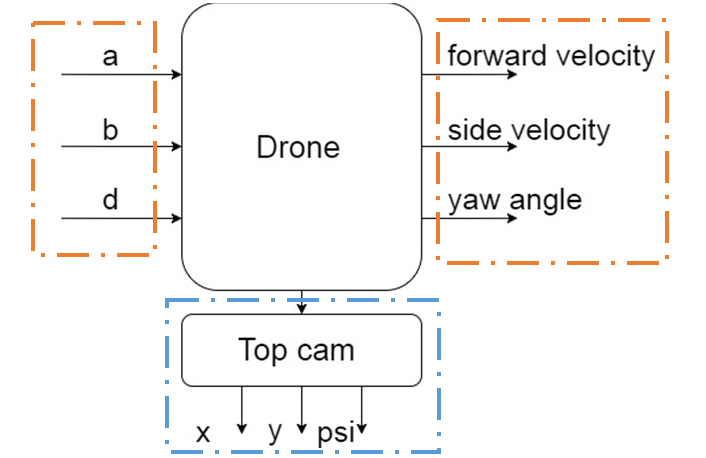
System identification and dynamic modeling
The model needed to be identified is the drone block in figure 1. The drone block in figure 1 is regarded as a black box. To model the dynamic of this black box, predefined signals are given as inputs. The corresponding outputs are measured by both top cam and velocity inside the drone. The relation between inputs and outputs are analyzed and estimated in following chapters.
Data preprocessing
As around 25% of the data measured by camera is empty, the drone positon information reflected is incomplete. The example (fig.2) provide a visualized concept of original data measured from top camera. Based on fig 2, the motion data indicted clearly what motion of drone is like in one degree of freedom. To make it continuous, interpolation can be in implemented.
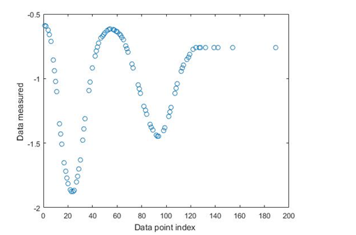
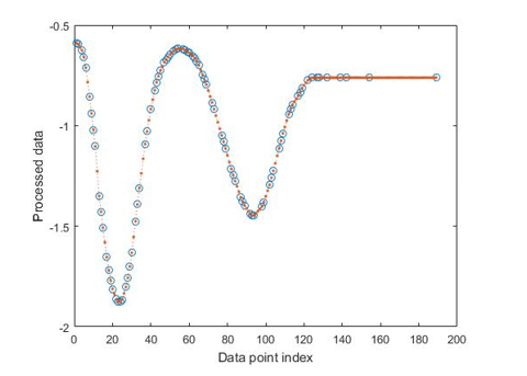
The processed data shows that the interpolation operation estimates reasonable guess for empty data points.
2.2 Coordinates system introduction
As the drone is flying object with four degree of freedom in the field, there exist two coordinate systems. One is the coordinate system in body frame, the other one is the global frame.
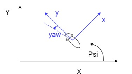
The drone is actuated in body frame coordinate system via control signals (a, b, c, d). The velocities measured are displayed also in the body frame coordinate system. The positions measured by the top camera are calculated in global coordinate system.
The data can be transformed between body frame and global frame via the rotation matrix. To simplify the identification process, the rotation matrix will be build outside the kalman filter. The model identified is the response of the input commends (a, b, c and d) in body frame. Then the filtered data will be transferred back to global frame as feedback. The basic concept is filtering data in body frame to avoid make parameter varying kalman filter. Figure 5 describes the basic concept in block diagram.
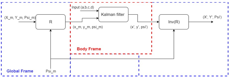
2.3 Model identification from input to position
The input and corresponding output in velocity in decoupled in body frame theoretically. Therefore, the dynamic model can be identified for each degree of freedom separately.
System identification for b (drone left-right tilt)
The response of input b is measured by the top camera. The preprocessed data is shown in following. And this processed data will be used in model identification.
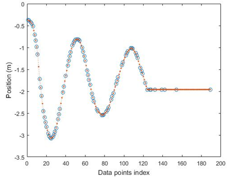
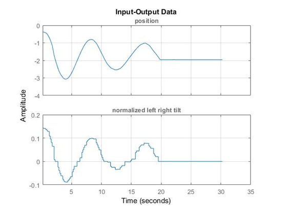
The above displays the input and corresponding output. System Identification Toolbox in MATLAB is used to estimate mathematical model with data shown above. As in real world, nothing is linear due external disturbance and components uncertainty. Hence, some assumptions need to be made to help Matlab make a reasonable estimation of model. Base on the response from output, the system behaves similar to a 2nd system. The states name is defined asX= [x ̇ x], which means velocity and positions. And identified model is demonstrated in state- space form: [EQUATION 1] The frequency response based on this state space model is shown below:
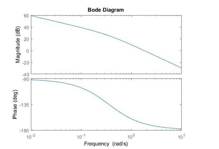
The accuracy of the identified model compared with real response is evaluated in Matlab. The result represents the extent about how the model fits the real response.
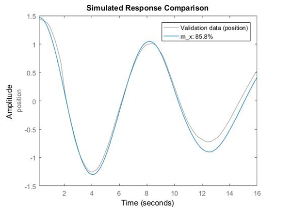
Data analysis
The model is built under the assumption that there is no delay from the inputs. However, according to the Simulink model built by David Escobar Sanabria and Pieter J. Mosterman, they measured and built the model of AR drone with 4 samples delays due the wireless communication. Compared with the results measured several times, the estimation is reasonable.
In real world, nothing is linear. The nonlinear behavior of system may cause the mismatch part of the identified model.
Summary
The model for input b, which will be used for further kalman filter design, is estimated with a certain accuracy. But the repeatability of the drone is a critical issue which has been investigated. The data selected for identification is measured in situation that battery is full, the orientation is fixed and no drone started from steady state.
System identification for a (drone front-back tilt)
The identified model in y direction is described as a state space model with the state name [(y ) ̇y] which means velocity and position.
The model then is:
[EQUATION 2]
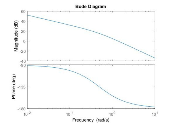
Estimator
To reduce the false positive detections and required processing work; some a priori knowledge about the objects to be detected is necessary. For example in case of circle detection the expected diameter of the circles is important. In that manner, the following estimator functions are defined as part of the World Model
The estimator blocks which defined are ball size, object size and line estimators. Using the recent state of the drone and information about the field of view of the camera and resolution (which are defined in initialization function); these estimators generate settings for the line, ball and object detection algorithms to reduce the false positives, errors and processing time of the algorithms.
Ball Size Estimator
Ball Detection Skill is achieved using imfindcircle built-in command of the image processing toolbox of MATLAB®. To run this function in an efficient way and reduce the false positive ball detections, the expected radius of the ball as the unit of pixels in the image should be defined. This can be calculated via the available height information of agent which carries the camera, field of view of the camera and the real size of the ball. The height information is obtained from the drone position data and the others are defined in the initialization function. The obtained estimated ball radius in pixel units is calculated here and fed into the ball detection skill.
Object Size Estimator
Very similar to the ball case, the expected size of the objects in pixels are estimated using the drone height and FOV. Instead of the ball radius, here the real size of the objects are defined. The obtained estimated object radius in pixel units is fed into the object detection skill.
Line Estimator
Line Estimator block gives the expected outer lines of the field. This estimator always calculates the relative position of the outer lines corresponding the state of the drone. This position information is coded using Hough Transformation criteria. The line estimator is required for enabling and disabling of the line detection on the outer lines. If some of the Outer Lines are in the field of view of the Drone Camera, then the Line Detection Skill should be enabled. Otherwise should be disabled. This information is also coded in the output matrix of the functional block. Because an always running Line Detection skill will produce many positive detected line outputs. The expected positions of the outer lines are not only used for enabling-disabling of the Line Detection Skill. Since the relative orientation and position of the lines are computable, this information is also used to filter out the false positive results of the line detection when it is enabled. The filtered lines then will be used for Refereeing Task.
The more detailed information and algorithm behind this estimator is explained here. However, an additional column is added to the output matrix of the Line Estimator function to show whether the predicted line is an end or side line.
Hardware
Drone
In the autonomous referee project, commercially available AR Parrot Drone Elite Edition 2.0 is used for the refereeing issues. The built-in properties of the drone that given in the manufacturer’s website are listed below in Table 1. Note that only the useful properties are covered, the internal properties of the drone are excluded.
The drone is designed as a consumer product and it can be controlled via a mobile phone thanks to its free software (both for Android and iOS) and send high quality HD streaming videos to the mobile phone. The drone has a front camera whose capabilities are given in Table 1. It has its own built-in computer, controller,accelerometers,altimeter, driver electronics etc. Since it is a consumer product, its design, body and controller are very robust. Therefore, in this project, the drone own structure, control electronics and software are decided to use for positioning of the drone. Apart from that, the controlling of a drone is complicated and is also out of scope of the project.
Experiments, Measurements, Modifications
Swiveled Camera
As mentioned before, the drone has its own camera and this camera is used to catch images. The camera is placed in front of the drone. However for the refereeing, it should look to the bottom side. Therefore the first idea was disassembling it and connecting the camera to a swivel to tilt down 90 degrees. This will cause some change in the structures. Since all the implementation is achieved using MATLAB/Simulink environment, the images of the camera should be reachable by MATLAB environment. However, after some effort and trial and error processes, it is observed that capturing and transferring the images of the drone embedded camera is not easy or straightforward for MATLAB. Even more effort showed that, the use of this drone camera for capturing images is either not compatible with MATLAB or causes a lot of delay. Therefore the idea of swiveled drone camera is abandoned and a new camera system is investigated.
Software Restrictions on Image Processing
Using a commercial and non-modifiable drone in this manner brings some difficulties. Since the source code of the drone is not open, it is very hard to reach some data on the drone including the images of the camera. The image processing will be achieved in MATLAB. However, taking snapshots from the drone camera directly using MATLAB is not possible with its built-in software. Therefore an indirect way is required and this causes some processing time. The best time obtained with the current capturing algorithm is 0.4 Hz using 360p standard resolution (640x360). Although the camera can capture images with higher resolution, processing will be achieved using this resolution to decrease the required processing time.
FOV Measurement of the Drone Camera
One of the most important properties of a vision system is the field of view (FOV) angle. The definition of the field of view angle can be seen in the figure. The captured images has a ratio of 16:9. Using this fact and after some measurements, the achieved measurements showed that it is near to 70° view although given that the camera has 92° diagonal FOV. The achieved measurements and obtained results are summarized in Table 2. Here corresponding distance per pixel is calculated in standard resolution (640x360).
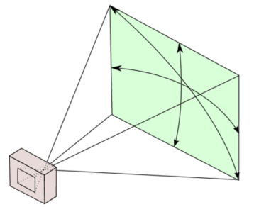
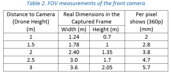
Although these measurement are achieved using drone camera, it is not used for the final project because of the difficulty on the getting images using MATLAB. Instead, an alternative camera system is investigated. To be able to have an easy communication and satisfactory image quality, a TCP/IP interface communication-based WiFi camera is selected. This camera is called as AiBall and it is explained in the following section.
Initialization
The following properties have to be initialized to be able to use the drone. For the particular drone that is used during this project, these properties have the values indicated by <value>:
- SSID <ardrone2>
- Remote host <192.168.1.1>
- Control
- Local port <5556>
- Navdata
- Local port <5554>
- Timeout <1 ms>
- Input buffer size <500 bytes>
- Byte order <litte-endian>
Note that for all properties to initialize the UDP objects that are not mentioned here, MATLAB's default values are used.
After initializing the UDP objects, the Navdata stream must be initiated by following the steps in the picture below.
Finally, a reference of the horizontal plane has to be set for the drone internal control system by sending the command FTRIM. [1]
Wrapper
As seen in the initialization, the drone can be seen as a block with expects a UDP packet containing a string as input and which gives an array of 500 bytes as output. To make communicating with this block easier, a wrapper function is written that ensures that the both the input and output are doubles. To be more precise, the input is a vector of four values between -1 and 1 where the first two represent the tilt in front (x) and left (y) direction respectively. The third value is the speed in vertical (z) direction and the fourth is the angular speed (psi) around the z-axis. The output of the block is as follows:
- Battery percentage [%]
- Rotation around x (roll) [°]
- Rotation around y (pitch) [°]
- Rotation around z (yaw) [°]
- Velocity in x [m/s]
- Velocity in y [m/s]
- Position in z (altitude) [m]
Top-Camera
The top camera is a wide angle camera that is fixed above the playing field and able to see the whole field.
This camera is used to measure the location and orientation of the drone. This measurement is used as feedback for the drone to position itself to the desired location.
The ‘GigeCam’ toolbox of MATLAB® is used to communicate with this camera. To obtain the indoor position of drone, 3 ultra-bright LEDs are placed on top of the Drone. A snapshot image of the field together with the agent is taken with a short exposure time. Then via the processing of this image for searching the pixels illuminated by the LEDs on the Drone, the coordinates on x and y-axes are obtained. Also, the yaw (ψ) orientation of the drone is obtained according to the relative positions of the pixels.
The top-cam can stream images with a frame rate of 30 Hz to the laptop, but searching the image for the drone (i.e. image processing) might be slower. This is not a problem since the positioning of the drone itself is far from perfect and not critical as well. As long as the target of interest (ball, players) is within the field of view of the drone, it is acceptable.
Ai-Ball : Imaging from the Drone
As a result of the searches, we finally decided to use a Wi-fi webcam whose details can be found here. This solution is a low-weight solution that sends images directly using a wifi connection. To be able to connect the camera, one needs a Wi-Fi antenna. The camera is placed faced down and in front of the drone. To reduce the weight of the added system, the batteries of the camera is removed and its power is supplied by drone using a USB power cable.
The camera is calibrated using a checker-board shape. The calibration data and functions can be found in the Dropbox folder.
One of the most important properties of a camera is the field of view (FOV) of the camera. The definition of the FOV is shown above. The resolution of the AiBall is 480p with 4:3 aspect ratio. This yields 640x480 pixels image.
The diagonal FOV angle of the camera is given as 60°. This information is necessary to know the real world size of the image frame and the corresponding real dimension of the per pixel. This information is embedded into Simulink code while converting measured positions to world cooordinates.
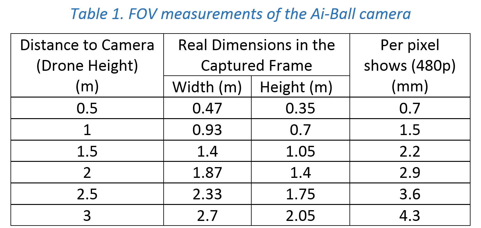
TechUnited TURTLE
Originally, the Turtle is constructed and programmed to be a football playing robot. The details on the mechanical design and the software developed for the robots can be found here and here respectively.
For this project it was to be used as a referee. All the software that has been developed at TechUnited did not need any further expansion as some part of the extensive code could be used to fulfill the role of the referee. This is explained in the section Software/Communication Protocol Implementation of this wiki-page.
Drone Motion Control
The design of appropriate tracking control algorithms is a crucial element in accomplishing the Drone referee project. The agents in this projects have two main capabilities which allow them to move and take images. With regards to situation of a game and the agents position, the desired position of each agents are calculated based on the subtask that is assigned to them. Generating the reference point is within the responsibilities of path-planning block which is not covered here. The goal of the Motion control block for the drone is to track effectively the desired drone states (xd,yd,θd) which represent the drone position and yaw angle in global coordinate system. These values as an outputs of path planning block are being set as a reference value for motion control block. As it is shown in Fig.1, the drone states obtained from a top camera which is installed on the ceiling to use as feedback in control system. The drone height z also should be maintained at a constant level to provide suitable images for image processing block. In this project, planar motion of the drone in (x,y) is interested as the ball and objects in pitch move in 2-D space. Consequently, the desired trajectories of drone are trajectories like straight line while performing aggressive acrobatic maneuvers are not interested. Hence, linear controllers can be applied for tracking planar trajectories.
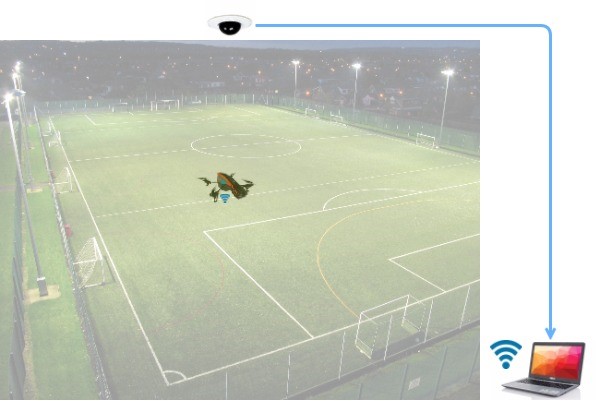
Most linear control strategies are based on a linearization of the nonlinear quadrotor dynamics around an operating point or trajectory. A key assumption that is made in this approach, is that the quadrotor is subject to small angular maneuvers. As it is shown in fig. 2, drone states (x,y,θ) that are measured by the images from the top camera are compared to the reference values. The high level controller (HLC) then calculates the desired speed of the drone in global coordinate and sends it as an input to the speed controller of the drone that is Low Level Controller (LLC). In this project, HLC is designed and the parameter are tuned to meet a specific tracking criteria. LLC is already implemented in drone. With identification techniques, the speed controller block was estimated to behave approximately as first order filter. Furthermore, incorporation of rotation matrix, the commands that are calculated in global coordinates, are transformed in to drone coordinates and being sent as a Fly commands to the drone.

At this level, the controller calculates the reference values of the LLC as an input based on the states errors that needs to be controlled (Fig.3). The input-output diagram of controller for each states are composed of 3 region. In dead zone region, if the error in one direction is less than a predefined value, then the output of the controller is zero. This result in comfort zone that the drone would stay without any motion which corresponds to the dead zone of the controller. If the error is larger than that value, then the output is determined based on the error and derivative of the error with PD coefficients (Fig.4). Since there is no position dependent force in the motion equation of the drone, I action is not necessary for controller. Furthermore, to avoid the oscillation in unstable region of the LLC built in the drone, the errors out of the dead zone region haven’t been offset from the dead zone region. This approach prevent sending small commands in the oscillation region to the drone.
High Level & Low Level Controllers
At this level, the controller calculates the reference values of the LLC as an input based on the states errors that needs to be controlled (Fig.3). The input-output diagram of controller for each states are composed of 3 region. In dead zone region, if the error in one direction is less than a predefined value, then the output of the controller is zero. This result in comfort zone that the drone would stay without any motion which corresponds to the dead zone of the controller. If the error is larger than that value, then the output is determined based on the error and derivative of the error with PD coefficients (Fig.4). Since there is no position dependent force in the motion equation of the drone, I action is not necessary for controller. Furthermore, to avoid the oscillation in unstable region of the LLC built in the drone, the errors out of the dead zone region haven’t been offset from the dead zone region. This approach prevent sending small commands in the oscillation region to the drone.
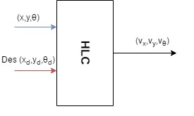
It should be noted that, these errors are calculated with respect to the global coordinate system. Hence, the control command first must be transformed in to drone coordinate system with rotational matrix that uses Euler angles.
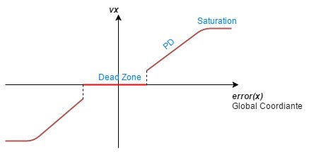
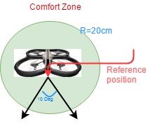
Coordinate System Transformation
The most commonly used method for representing the attitude of a rigid body is through three successive rotation angles (Ф,φ,θ) about the sequentially displaced axes of reference frame. These angles are generally referred to as Euler angles. Within this method, the order of rotation around the specific axes is of importance as the sequence of rotations. In the field of automotive and/or aeronautical research, the transformation from a body frame to an inertial frame is commonly described by means of a specific set of Euler angles, the so-called roll, pitch, and yaw angles (RPY). In this project, since the motion in z-direction is not subject to change and the variation in the pitch and roll angles are small, then the rotation matrix reduced to function of yaw angle.
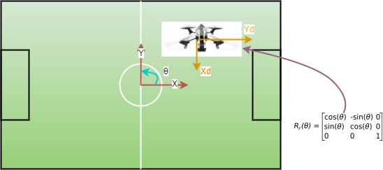
Player
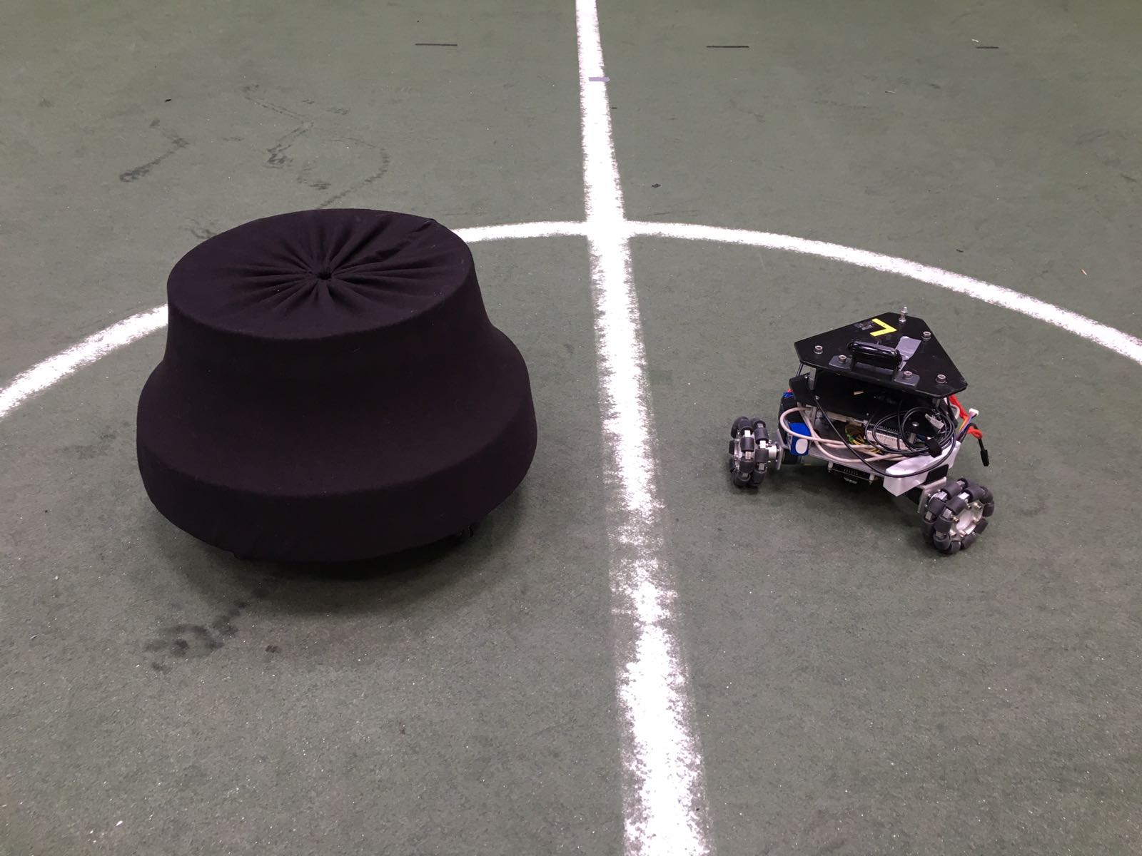
The robots that are used as football players are shown in the picture. In the right side of the picture, the robot is shown as it was delivered at the start of the project. This robot contains a Raspberry Pi, an Arduino and three motors (including encoders/controllers) to control three omni-wheels independently. Left of this robot, a copy including a cover is shown. This cover must prevent the robots from being damaged when they are colliding. Since one of the goals of the project is to detect collisions, it must be possible to collide more than once.
To control the robot, Arduino code and a Python script to run on the Raspberry Pi are provided. The python script can receive strings via UDP over Wi-Fi. Furthermore, it processes these strings and sends commands to the Arduino via USB. To control the drone with a Windows device, MATLAB functions are implemented. Moreover, an Android application is developed to be able to control the robot with a smartphone. All the code can be found on GitHub.[2] >
Supervisory Blocks
Integration
As explained in System Architecture part, the project consists of many different subsystems and components. Each component has its own task and functions. All of these tasks and skills are implemented using the built-in Matlab® functions and libraries. Communication between all the components is required to apply communication, queuing and ordering according to the tasks and project aims. Regarding tasks and functions; some of the processings and functions are required to work simultaneously, some are consecutive and some others are independent. Additionally, the implementation of the system should also be compatible with system architecture. As you can see in the system architecture, the design has layers. To handle the simultaneous communication and layered structure, Simulink software is used for programming. In that sense, the Simulink diagram created for the project is given in the following figure.
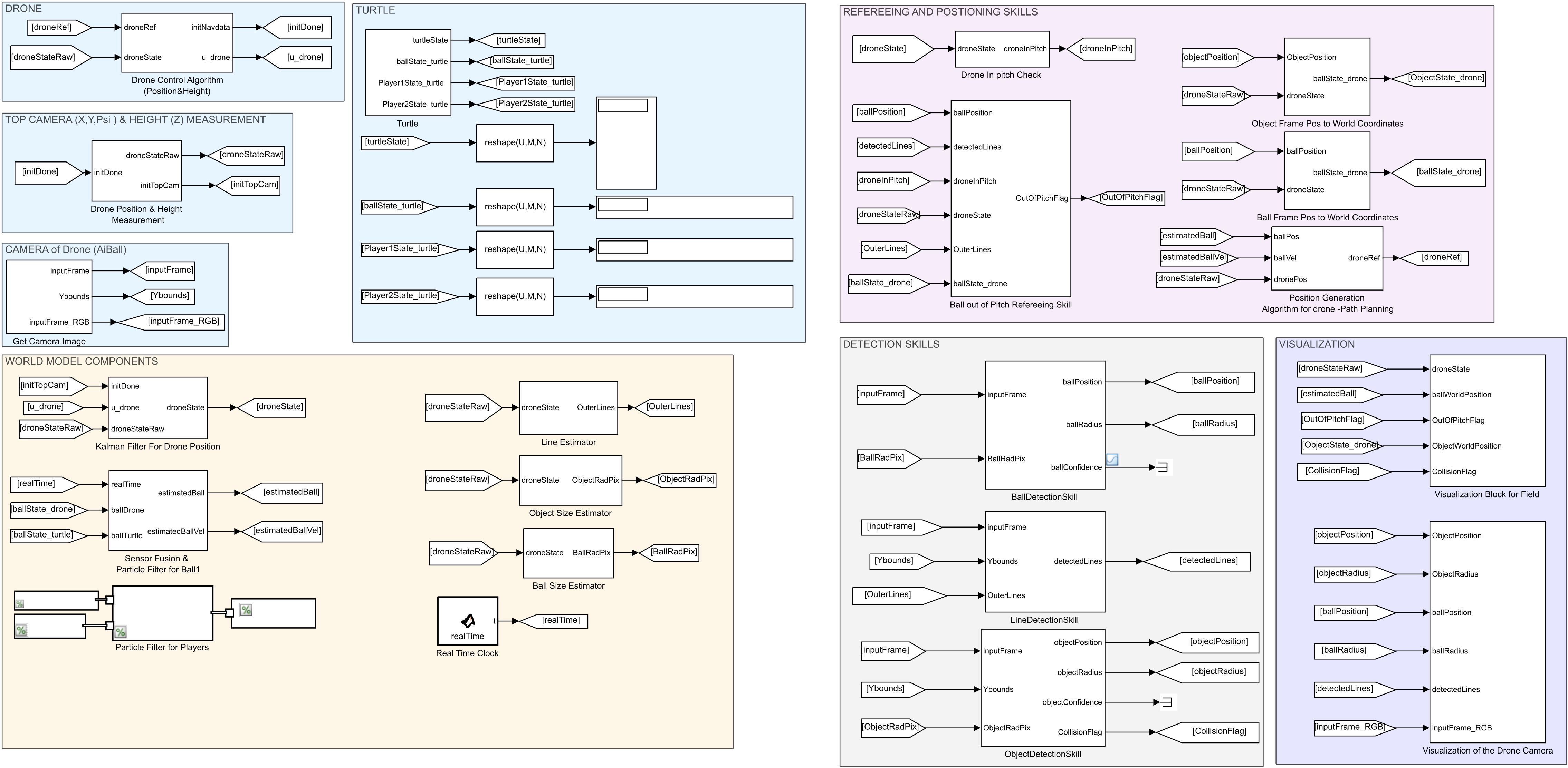
Properties of the Simulink File
- In Simulink diagram, blocks are categorized using Area utility, according to the functions/tasks that they have.
- The categorization is shown via different colors and these divisions are consistent with the system architecture.
- The interconnections between the functioning blocks are achieved via GoTo and From functions and transferring parameter names are shown explicitly.
- Each individual blocks and their function in this Simulink diagram is explained in these documentations.
- All the functions and blocks under Visualizations area are not part of the main tasks of the project but are necessary to see the results. Therefore this part is not part of the System Architecture.
- Since almost the all functions and built-in commands in the algorithms are not directly available to Simulink, each Matlab function is called from Simulink using extrinsic command.
- The blocks, functions and developed codes are well commented. The details of the algorithms can be examined while examining the source codes.
Hardware Inter-connections
The Kinect and the omni-vision camera on the TechUnited Turle allow the robot to take images of the on-going game. With image processing algorithms useful information from the game can be extracted and a mapping of the game-state, i.e.
1. the location of the Turtle,
2. the location of the ball,
3. the location of players
and other entities present on the field can be computed. This location is with respect to the global coordinate system fixed at the geometric center of the pitch. At TechUnited, this mapping is stored (in the memory of the turtle) and maintained (updated regularly) in a real-time data-base (RTDb) which is called the WorldMap. The details on this can be obtained from the software page of TechUnited. In a Robocup match, the participating robots, maintain this data-base locally. Therefore, the Turtle which is used for the referee system, has a locally stored global map of the environment. This information was needed to be extracted from the Turtle and fused with the other algorithms and software that was developed for the drone. These algorithms and software were created on MATLAB and Simulink while the TechUnited software is written in C and uses Ubuntu as the operating system. The player-robots from TechUnited, communicate with each other via the UDP communication protocol and this is executed by the (wireless) comm block shown in the figure that follows.
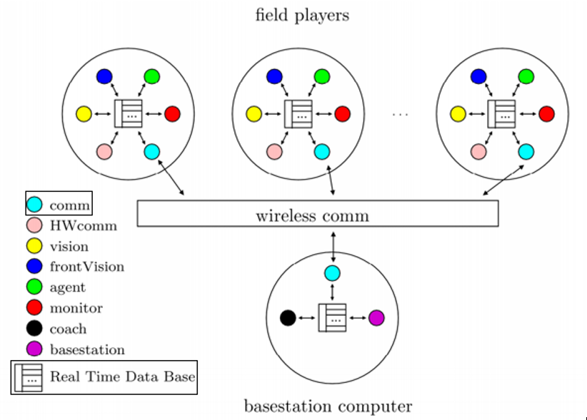
The basestation computer in this figure is a DevPC (Development PC) from TechUnited which is used to communicate (i.e. send and receive date) with the Turtle. Of all the data that is received from the Turtle, only a part of it was handpicked as it suited the needs of the project the best. This data, as stated earlier is information on the location of the turtle, the ball and the players.
A small piece of code from the code-base of TechUnited was taken out. This piece consisted of functions which extracted the necessary information from the outputs generated by image processing running on the Turtle by listening to this information through the S-function sf_test_rMS_wMM.cItalic text created in MATLAB’s environment and sent to the main computer (running on Windows) via the UDP Send and UDP Receive block in Simulink.
This is figuratively shown in the picture below.
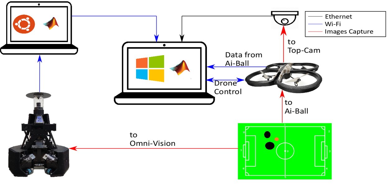
The s-function behind the communication link between the Turtle and the Ubuntu PC was implemented in Simulink and is depicted as follows. The code can be accessed through the repository.