Viotar/Model: Difference between revisions
No edit summary |
|||
| (3 intermediate revisions by 2 users not shown) | |||
| Line 26: | Line 26: | ||
[http://cstwiki.wtb.tue.nl/index.php?title=Viotar Main page] | [http://cstwiki.wtb.tue.nl/index.php?title=Viotar Main page] | ||
[http://cstwiki.wtb.tue.nl/index.php?title=Viotar/ | [http://cstwiki.wtb.tue.nl/index.php?title=Viotar/Working_of_the_violin Working principle of the violin and predicting it’s behavior] | ||
[http://cstwiki.wtb.tue.nl/index.php?title=Viotar/_Ways_To_Exite_The_String Ways to exite the string] | |||
[http://cstwiki.wtb.tue.nl/index.php?title=Viotar/ | [http://cstwiki.wtb.tue.nl/index.php?title=Viotar/Hardware_Design Hardware Design] | ||
[http://cstwiki.wtb.tue.nl/index.php?title=Viotar/Quantifying_the_signal Software Design (Quantifying the signal we want to see)] | [http://cstwiki.wtb.tue.nl/index.php?title=Viotar/Quantifying_the_signal Software Design (Quantifying the signal we want to see)] | ||
[http://cstwiki.wtb.tue.nl/index.php?title=Viotar/ | [http://cstwiki.wtb.tue.nl/index.php?title=Viotar/Patent_Research Patent Research] | ||
[http://cstwiki.wtb.tue.nl/index.php?title=Viotar/ | [http://cstwiki.wtb.tue.nl/index.php?title=Viotar/Background_information:_Interview_with_Hendrik_Zick Background information: Interview with Hendrick Zick] | ||
[http://cstwiki.wtb.tue.nl/index.php?title=Viotar/Model Model] | [http://cstwiki.wtb.tue.nl/index.php?title=Viotar/Model Model] | ||
| Line 127: | Line 127: | ||
[[File:HEL.PNG|frame|border|center|Figure 7: Helmholtz vibration and it's powerspectrum]] | [[File:HEL.PNG|frame|border|center|Figure 7: Helmholtz vibration and it's powerspectrum]] | ||
====Region of Helmholtz motion in parameter space==== | ====Region of Helmholtz motion in parameter space==== | ||
Latest revision as of 16:31, 25 January 2011
ModelIn order to predict the results of experiments for validation and to make the designing of the controller more easy, a model of the vibration of a bowed string will be made. This model is made in matlab and will be discussed in the following chapter. Friction curve modelSimple approximationIn simple models of the interaction between bow and string, it is asumed that the friction force between both only depends on the relative speed of the string in relation to the bow. The relation between the relative speed and friction force has an exponential shape in these models. This can also be seen in figure 3. In this figure v is the speed of the string, where vb is the bowing speed. The friction force on the interaction area of the bow and the string, can be calculated using: [math]\displaystyle{ f = \mu(v-v_b)f_b }[/math] Where µ is the friction coefficient and fb is the applied force on the bow. 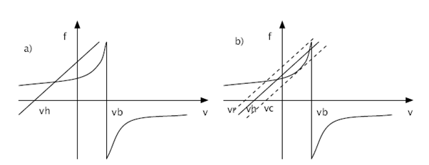 There are several models for the friction coefficient µ. The hyperbolic model is described as follows: [math]\displaystyle{ \mu = \mu_d + {{(\mu_s-\mu_d)v_0} \over {v_0 + v + v_b}} }[/math] where: vo = initial bowing speed µd = dynamic friction coefficient µs = static friction coefficient (In most cases, the values µd = 0.3 and µs = 0.8 are used)
[math]\displaystyle{ \mu = 0.4e^{{v-v_b}\over{0.01}} + 0.45e^{{v-v_b}\over{0.1}} + 0.35 }[/math] 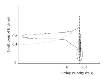 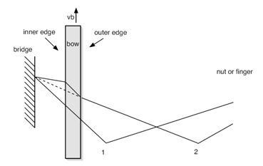 In figure 3, also the relation between applied force and caused velocity of the string is shown. This dynamical behaviour of the string is approximately linear, as experiments proved. The release velocity vr and capture velocity vc are shown in figure 3 b). The are the velocities at which the string respectively slips of the bow or sticks on it. This phenomenon can be explained as follows. When the velocity of the string increases, the string keeps slipping on the bow until the capture velocity is reached. At this velocity the string sticks on the bow and therefor has the same velocity. The string will remain sticking until the release velocity is reached. At that point, the string starts slipping over the bow. This means that the force equation has a different solution when the relative speed increases than it has when the relative speed decreases. This is due the fact that the friction coefficient for slipping differs from the friction coefficient for sticking. Friction model vs. ExperimentIn the simple friction curve model, like it is presented in figure 3, it is assumed that the friction force only depends on the relative force between the string and the bow. However, experiments have proved that the true situation is not quite as simple as that. The dotted line in figure 4 shows the relation between string velocity and friction coefficient as described by the model above. The continuous line shows the real situation, which has been measured experimentally. From this figure it can be concluded that the classical approach is quite unprecise. Explanations for errors in the friction modelOne of the reasons for this, is that the temperature of the interaction area is of very high importance. This is because of the melting temperature of the rosin. When the relative speed is low, the contact area cools down due to conductance in the string and bow. This causes the friction coefficient to increase. When more 'slip' behaviour occurs, this causes the temperature to raise and therefor the friction coefficient tot decrease rapidly. Another phenomenon that turns out to have a lot of influence, is the so called hair-compliance. This error is occured by the fact that the bow doesn't have one single contact point with the string (like assumed in the simple model), but in fact has a whole contact area. The difference is that for the first case it is possible to have absolutely no slip while the string follows the bow, while in the second case slip is always present. This difference is also shown in figure 5. In this figure, situation 1 indicates the initial string and bow. One time step later (situation 2) the bow has moved upwards with velocity vb and the string has sticked on the bow. Now, the dashed line represents the real situation, like it would be in realtity, where the continuous line indicates what shape the string should have as no slip had occured. It should be clear that this 'no slip situation' would never occur in reality and therefor bowing without any slip is impossible. However, experiments proved that the simple representation of the friction curve model is precise enough to simulate what the influence of changing the bowing speed and force is, on the occurence of a Helmholtz vibration. For our computer model we will use the friction curve, like it is presented in figure 3 which will satisfy. Computer modelVariabelsThere are 3 variables that can be set in this model. These are the bowing speed vb, bowing force fb and a factor that indicates the distance between the bow and the bridge and the bow, in relation to the length of the string (β). Working of the program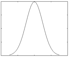 In the computer program, the simulation is devided into n intervals of size dt. The program runs through a loop for every time step dt. Using the known values (from earlier time steps)for position of the string, velocity of the string and applied force on the bow, new values for these quantities are calculated. Important is that the speed at which an applied force moves through the string, is known. With this structure it is always possible to calculate the new values on time i, using the values from the past. To illustrate the working of the program, one loop will be run through in the following part. The string will be evaluated at position x on time i. Vibrations caused at position x, will move along the string to the ends, where the vibrations are reflected to position x. On time i, the time is calculated at which the vibrations that arrive on time i where caused on position x. So, this is a moment in the past. Beacause the travelling time of the waves is usually not a multiple of dt, the real time should most of the time be interpolated between two values. Beacuse of the fact that vibrations that are nearly at position x are also important for the movement of position x, also these vibrations are taken into account. Using a symmetric Gauss curve (figure 6), the influence of these vibrations is calculated and added to the vibration that has exactly returned on time i. All these vibrations together are forces that influence the vibration (velocity) of position x. Using the friction curve model, this resulting force can be converted to a new string velocity. This gives the string velocity vi on time i. When this loop is run through for all time steps, there is a vector v which contains the string velocity for every time i. The position of point x can easily be calculated using this vector by integrating over the time steps dt. When the complete vibration of the string is known (postion as a function of time), a powerspectrum can be made using fourier transformation. This gives the amplitude ratios in the frequency domain. ProblemsThe biggest problem so far, is that the frequency of the vibration seems to be depending on the bowing speed and force. In reality this is not the case, and is the frequency only depending on the length and the width of the string. Varying the bowing speed and force, only changes the amplitude and therefor the loudness of the vibration in reality. This problem is most probably caused by another problem, being the stiffness of the string. This stiffness plays an important role in the vibration of the string as it adds another force to force equation. New computer modelSince the model we made did not satisfy the fact that frequency should not depend on bowing speed and force, we contacted an expert for help. This expert, J. Woodhouse from the Cambridge University, has done several studies about the behaviour of a bowed string. He helped us a lot by sending a model he made years ago for recognizing Helmholtz vibration. He also used this model to define the Helmholtz region as a function of bowing speed, applied force and β. We adapted and used this model for our controller and to do analysis of Helmholtz vibrations. Analysis with the new modelWith the right model a Helmholtz vibration can be generated. This vibration can be analysed afterwards using matlab. The model itself recognises if the generated vibration is a Helmholtz vibration or a noisy type of vibration. We took a Helmholtz vibration, which looks like the left figure below, and made an m-file that generates a fourier transformation of that vibration. The powerspectrum that was generated is shown in the right figure below. These type of figures will be very important later on as we will see in the chapter 'Software Design (Quantifying the signal we want to see)'. 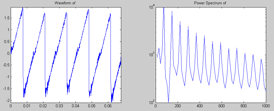 Region of Helmholtz motion in parameter spaceThe model has been run for a 20x20 grid of bowing speeds and bow forces. This has yielded the plot of Figure 7. 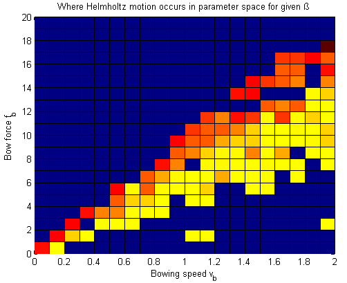 It’s interesting that there are exceptions to the main trend in the figure, that is, the “holes” in the Helmholtz region and the occurrences of Helmholtz outside the main region. This is strange because in a mathematical model, unlike in “reality”, there’s no noise or chaos. Probably, the reason why the results may be unpredictable is that these are not steady-state results, so there may still be startup phenomena. A way we may solve it in the future is to use “perfect transients”, in which Helmholtz motion is obtained within one period by following a certain acceleration path for the bow speed. Restrain should also be kept regarding the accuracy of the algorithm that “recognizes” if there is a Helmholtz vibration or not. Despite the inaccuracies, there is already valuable info in this plot. It becomes very clear “where” in the parameter space you want to be, as the lower part of the Helmholtz region has the smallest note flattening. When modulating the note intensity, the ideal path that should be taken would be somewhat like the green line drawn in Figure 8. 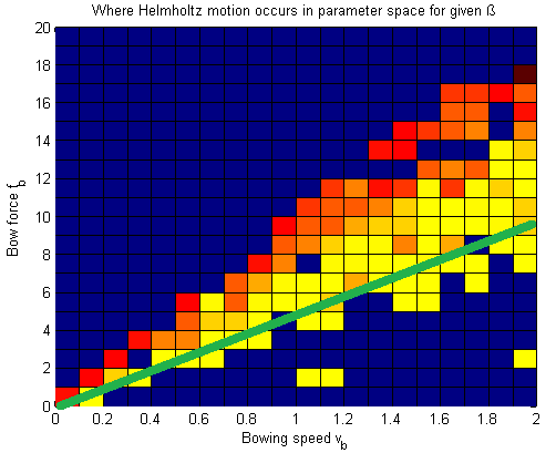 Adapting the model for the controllerThe model is a practical instrument for designing a controller. This gives the ability to design a controller without actually having the real prototype. Besides the advantage that both the prototype and the controller can be designed simultaneously, it also has the advantage that the influence of a certain input on the output can be checked very easily. This will also become clear in the chapter 'Software Design (Quantifying the signal we want to see)'. The model as we received from mr. Woodhouse, contains a loop to generate vibrations for varying β, bowing speed and force. To make the model suitable for the controller, we adapted it and removed the loop. The simulation model is a function that has bowing speed and force as input variables, while β is kept constant. We run this function file in simulink, where the input parameters can be changed on the fly. Every time step, the function is called, which calculates the new location of the simulated bowing point. This gives the ability to construct a controller which adapts the input variables for the function every time step. In this way, the model simulates the response of the guitar to certain input variables. |