Embedded Motion Control 2012 Group 7: Difference between revisions
| (113 intermediate revisions by 4 users not shown) | |||
| Line 1: | Line 1: | ||
<br><br> | |||
==Group Info== | ==Group Info== | ||
| Line 5: | Line 6: | ||
|'''Group Members''' - | |'''Group Members''' - | ||
|'''email''' (at student.tue.nl) | |'''email''' (at student.tue.nl) | ||
|- | |- | ||
| Siddhi Imming | | Siddhi Imming | ||
| s.imming | | s.imming | ||
|- | |- | ||
| Bart Moris | | Bart Moris | ||
| b.moris | | b.moris | ||
|- | |- | ||
| Roger Pouls | | Roger Pouls | ||
| r.c.e.pouls | | r.c.e.pouls | ||
|- | |- | ||
| Patrick Vaes | | Patrick Vaes | ||
| p.r.m.p.vaes | | p.r.m.p.vaes | ||
|- | |- | ||
|} | |} | ||
| Line 30: | Line 26: | ||
Rob Janssen - R dot J dot M dot Janssen at tue dot nl | Rob Janssen - R dot J dot M dot Janssen at tue dot nl | ||
<br><br> | |||
==Planning== | ==Planning== | ||
| Line 46: | Line 43: | ||
<tr><td>Week 10/11 (25 jun / 2 jul)</td><td>Final competition.</td><td><td></tr> | <tr><td>Week 10/11 (25 jun / 2 jul)</td><td>Final competition.</td><td><td></tr> | ||
</table> | </table> | ||
<br><br> | |||
== | ==Goals== | ||
Our main goal is to be able to solve the maze Jazz we will be faced with during the final competition. As the philosophy in the world of robotics and also behind the ROS platform is to share knowledge and to use knowledge of others in order to speed up the design process. Of course, we take care of not just plugging in some code designed by others without really understanding what is going on and on what principles the process is based on. So our focus will be on designing a robust and fast navigation algorithm, rather than designing all kinds of new implementations of really nice functions that are already available for ROS. | |||
<br><br> | |||
==Program structure== | |||
[[File:Programstructure.png|thumb|none|600px]]<br> | |||
The scheme above shows the first proposal of the components of which the final program will consist. A more detailed overview will be published in the coming days or week(s). The components in grey are considered to be not very important in order to successfully complete the corridor competition. However, these components are necessary for a successful completion of the final competition. | |||
'''Final structure''' | |||
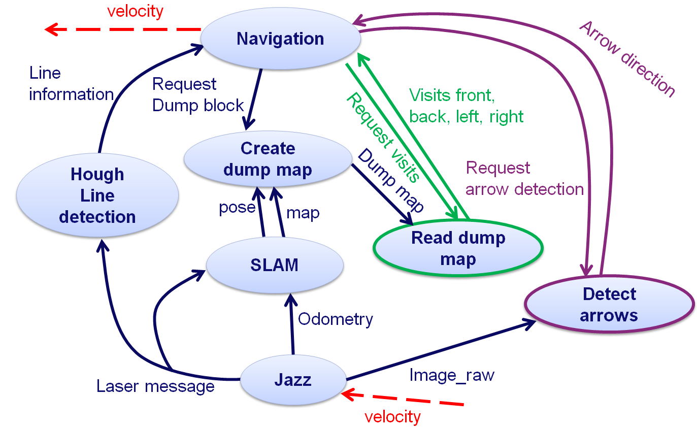
The final structure of the program is slightly different to the one shown above which was basically the outcome of our first brainstorm. Our current structure is shown below, where the oval shapes reperesent the node and the ones with a thick, coloured (but not blue) border are services. The navigation node actually does the navigation task and sends the velocity commands to Jazz in order to let it drive forward. Furthermore it recognizes exits and does the normal driving between two parallel walls. The node called "create dump map" constructs a map that counts the number of visits of each corridor in order to be able to perform the Tremaux's algorithm. The SLAM node is actually the gmapping node which is used to do simultaneous self-localization and mapping. Arrow detection is done by the service "Detect Arrows" and the node Hough Linedetection is used to detect walls and also an opening in a wall. Looking up the number of visits from the dumpmap is done by the service "Read dump map". | |||
[[File:Final_structure.png|thumb|none|600px]]<br><br> | |||
==Maze solving Algorithm's== | ==Maze solving Algorithm's== | ||
| Line 104: | Line 66: | ||
===Tremaux's Algorithm=== | ===Tremaux's Algorithm=== | ||
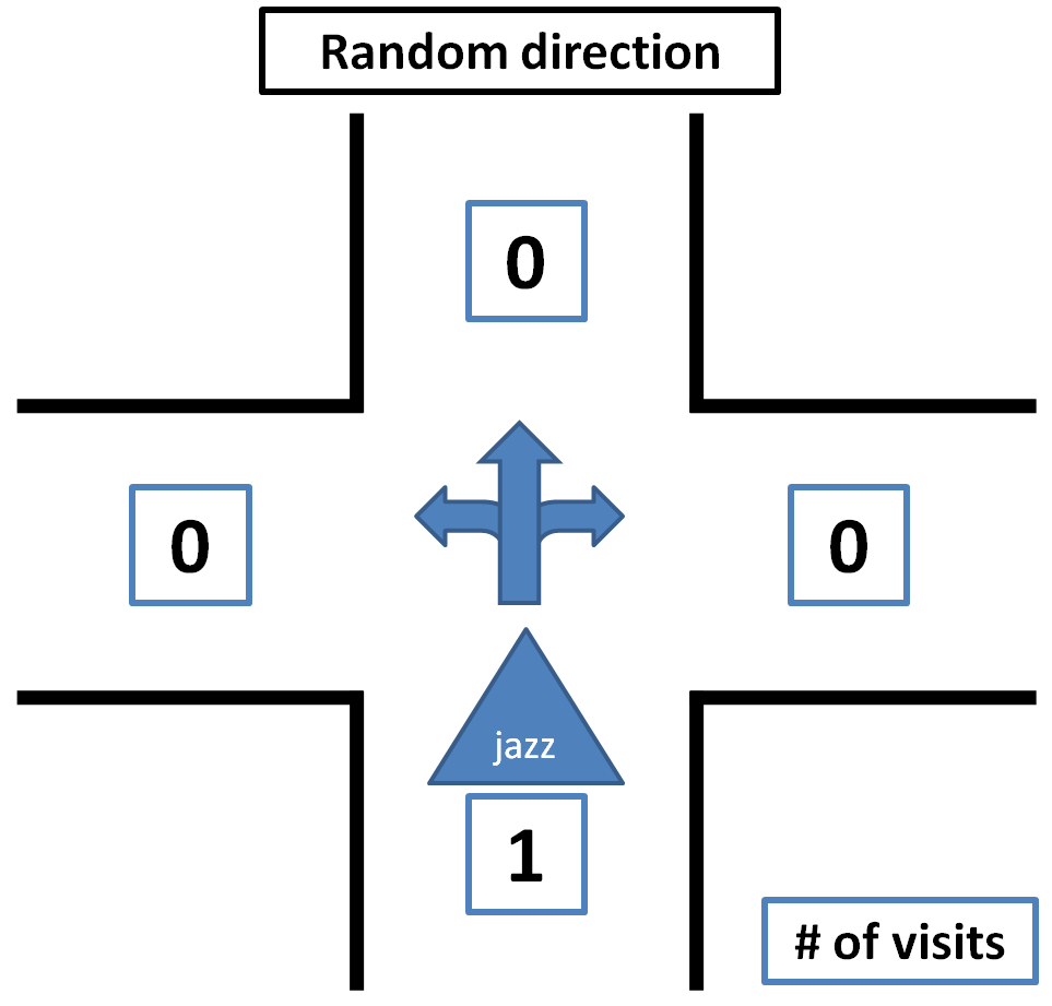
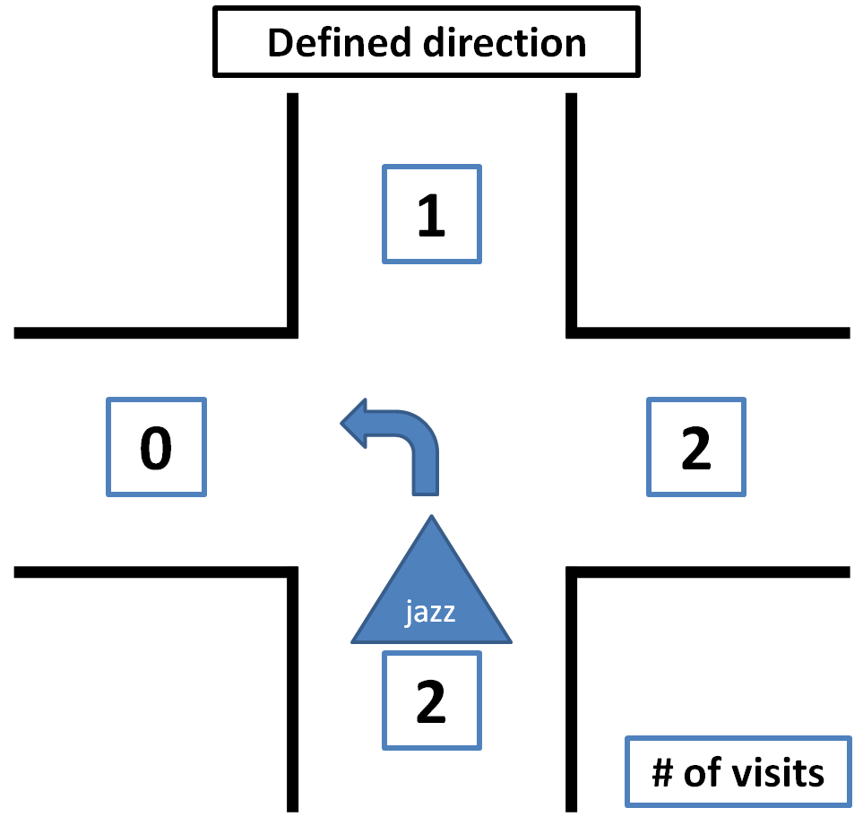
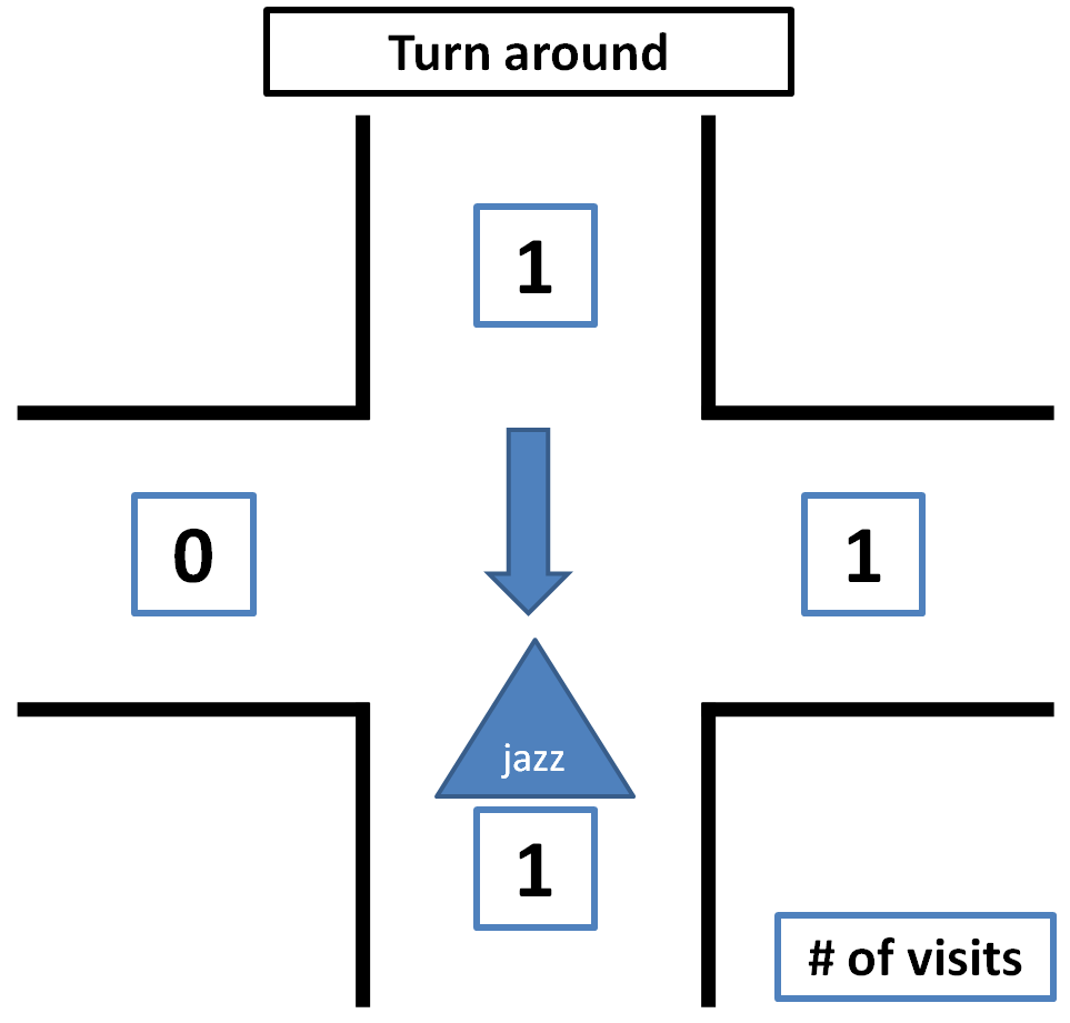
The Tremaux's Algorithm solves a maze by marking how many time a passage has been passed, when a junction is encountered that is not visited yet a random passage is chosen. If the junction is visited before the passage with the lowest counts of visits is chosen (if there are multiple options a random choice between these options is made). Exception to this is if the passage which we are arriving from is only visited once, then we will go back through the same passage, this is to avoid going around in circles. <br> | The Tremaux's Algorithm solves a maze by marking how many time a passage has been passed, when a junction is encountered that is not visited yet a random passage is chosen. If the junction is visited before the passage with the lowest counts of visits is chosen (if there are multiple options a random choice between these options is made). Exception to this is if the passage which we are arriving from is only visited once, then we will go back through the same passage, this is to avoid going around in circles. <br> | ||
Some pictures that clarify how the decision making is done by Tremaux's Algorithm are shown below.<br> | |||
<center> | |||
{| | |||
|[[File:Tremauxrandom.png|thumb|none|300px]] | |||
|[[File:Tremauxdefined.png|thumb|none|300px]] | |||
|[[File:Tremauxturnaround.png|thumb|none|300px]] | |||
|} | |||
</center> | |||
<br> | |||
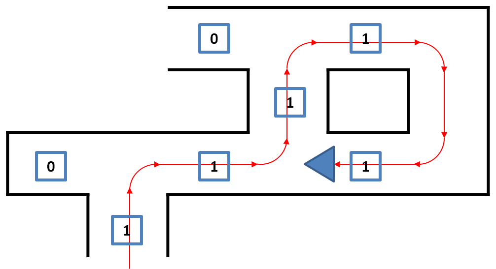
An example of why there has to be turned around at a junction at certain conditions is shown below. If at this point there is not decided to turn back, there is a change that the direction back to the beginpoint is chosen. <br> | |||
<center> | |||
[[File:Tremauxturnaroundwhy.png|thumb|none|450px]] | |||
</center><br> | |||
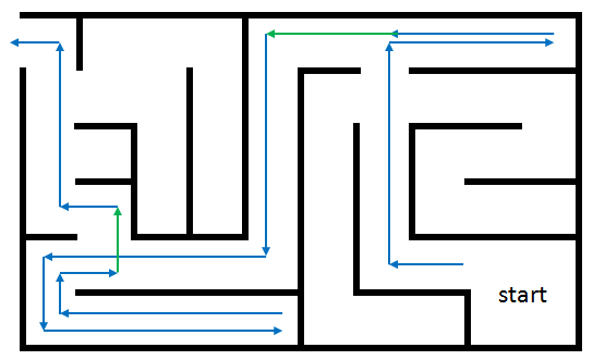
An example of a maze solved by the Tremaux's Algorithm is shown below, the green markers indicate a decision not made random but based on the number of visits of all the possible passages. | An example of a maze solved by the Tremaux's Algorithm is shown below, the green markers indicate a decision not made random but based on the number of visits of all the possible passages. | ||
<center> | <center> | ||
[[File:Solvetremaux.png|thumb|none|450px]]</center> | [[File:Solvetremaux.png|thumb|none|450px]]</center> | ||
<br> | <br><br> | ||
===Wall follower algorithm=== | ===Wall follower algorithm=== | ||
| Line 115: | Line 92: | ||
[[File:Solvewall.png|thumb|none|450px]]</center> | [[File:Solvewall.png|thumb|none|450px]]</center> | ||
==Navigation== | |||
===Line Detection=== | |||
To help Jazz driving straight through corridors and detecting junctions a line detection algorithm is implemented. The hough transform algorithm is the algorithm we have chosen for this, how this algorithm works and is implemented is explained here. | |||
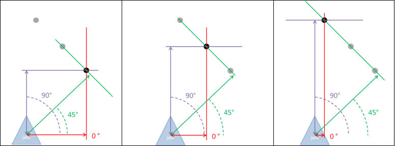
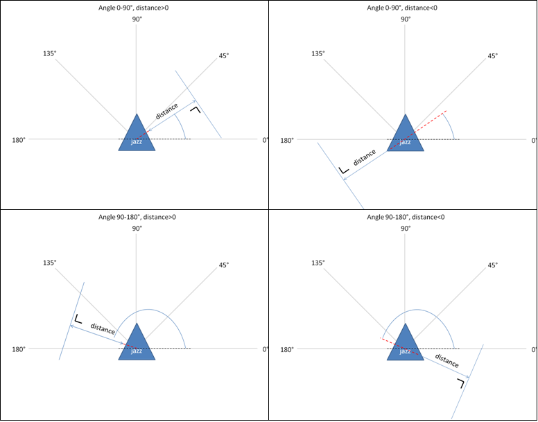
For every point that is detected by the laserscanner lines are drawn through that point with different angles, the distance perpendicular to the line is then measured. If for a certain angle the distances for two points are the same, these points are on the same line. This is further explained with some pictures. <br><br> | |||
<center> | |||
[[Image:Houghall.png|700px]]<br><br> | |||
[[Image:Houghpointstable.png|250px]] <br><br></center> | |||
From this example can be concluded that the points or on a line with angle 45° at a distance of 7. Of course in reality more lines per point are calculated depending on the required accuracy. Also the distance does never exactly match because of measurement noise and the fact that real walls are never perfectly straight. Therefore the distance does not have to be exactly the same but has to be within a certain tolerance. <br><br> | |||
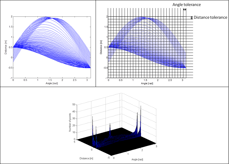
How this works for the real laserdata is explained with some pictures. First for every point the distance is plotted as a function of the angle. This angle goes from 0 degrees to 180 degrees in steps of the desired accuracy. This range can describe all possible lines like shown in the pictures below. <br><br> | |||
<center> | |||
[[Image:Linedefall.png|800px]] | |||
</center><br><br> | |||
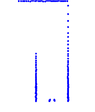
The implementation of this algorithm is now further explained with a captured frame of the laserdata shown below. | |||
<center> | <center> | ||
[[ | [[Image:Capturedlaserdata.png|200px]] | ||
</center> | </center> | ||
<br><br> | <br><br> | ||
First all the angles and distances for each point from the laserdata are calculated, then a raster is created with all possible lines. Each element of this raster represents a line with a certain angle and a certain distance to Jazz (measured perpendicular on the line). The size of the elements of this raster depends on the tolerances for the distance and angle that have been set. | |||
The number of points inside each element is counted. When the number of points is more than a certain threshold this is considered to be a line.<br><br> | |||
<center> | <center> | ||
[[Image:Houghexample.png|800px]] | |||
< | </center> | ||
< | <br><br> | ||
< | The first plot shows a graphical interpretation of all the lines that are calculated for each point. The second plot shows the raster and its elements, the points within each of these elements are counted. The elements which hold at least a certain amount of points represent a line, these are the peaks shown in the last figure.<br><br> | ||
< | '''Extraction of start and endpoints of the lines'''<br> | ||
< | The start and endpoints of a line are examined by appointing all the points from the laserscan to the lines the belong to. After this is done, two neighboring points are compared to see if there mutual distance is smaller than some tolerance in order to make sure that they lay on the same line section. For all the points belonging to one section, the first and last point are considered to be the start and endpoint of that particular section. The obtained information is sent to the navigation node which decides about the actions to take. The messages, defined by a new structure, that are sent by the line recognition node contain the number of lines, and for each line, the number of sections, and per section the coordinates of the begin and endpoint together with the number of points on the section. | ||
< | |||
< | ===Driving through corridor=== | ||
< | To drive safeley through a corridor without colliding into walls a corridor is virtually divided into 3 different zones. <br><br> | ||
< | ''Safe zone:'' <br> | ||
< | This zone is in the middle of the corridor and the desired velocity here will be at maximum allowed velocity, the desired driving direction of Jazz will be straight ahead. <br><br> | ||
< | ''Attention zone:''<br> | ||
< | These zones are a bit closer to the walls, therefore the desired velocity here will be half of the maximum allowed velocity, the desired driving direction will be slightly to the middle of the corridor to get into the safe zone again. <br><br> | ||
''Critical zone:''<br> | |||
These zones are so close to the wall that there is a severe risk of colliding with the walls. The desired velocity here will be set to zero if Jazz' driving direction is still directing to the wall. If the driving direction is directing from the wall the desired velocity will be half of the maximum allowed velocity. The desired driving direction will be pretty sharp to the middle of the corridor to leave the critical zone.<br><br> | |||
The zones are illustrated in the picture below.<br><br> | |||
<center> | |||
[[Image:Corridordriving.png|400px]] | |||
</center> | |||
===Junction handling=== | |||
< | In order to succesfully navigate through the maze, an appropriate junction handler has to be designed. In our opinion, the junction handling described below will do the job: | ||
There are basically 5 types of junctions Jazz will encounter during its drive through the maze as shown in the figure below. The red arrow indicates the direction from which Jazz approaches the junction. Note that a dead end is also considered to be and handeled is if it is a junction. | |||
< | <center> | ||
< | [[Image:Junctions.png|700px]] | ||
</center> | |||
The recognition of the different situations is planned to do in the following manner: | |||
# A junction is detected when a line at an angle of approximately 90 degrees is found, this line is referred to as an 'exitline'. | |||
# A line parallel to the side walls is drawn at the right end of this exitline, then the distance between this line (red dashed line in the image below) and the right wall is calculated. If this distance is larger than a certain tresshold, a right exit exists. | |||
# This is also done on the left side. | |||
# To check for front exits a line is drawn parallel to the exitline at the end of the lines at the side walls. The distance between this line and the exitline is calculated and if this distance is larger than a certain tresshold, a front exit exists. | |||
# Based on which exits are found the situation is determined. | |||
<center> | |||
[[Image:Exitdetection.png|400px]] | |||
</center> | |||
Based on the junction type detected, the appropriate action should be taken, such as drive forward, turn left/right, check for an arrow and check each passage for the number of visits. | |||
'''Robustness Measures''' | |||
In order to make the junction recognition robust and also working in case of minor deviations from the ideal situation we have taken some measures. The most important measures are explained below. Note that these are additions to the original proposed method, as this method worked fine in ideal cases but not for a whole maze with a seris of junctions connected to each other. | |||
* Paralell lines which are used by Jazz to recognize the walls between which it drives are limited to a distance of 1 meter, in order to make the right distinction between for example a corner and a dead end in case of coupled junctions. | |||
* If only one side wall is detected, the previously measured hallwidth is used to approximate the position of the other side wall. | |||
* Decisions are made only after one type of exit is recognized 2 times, to prevent Jazz from taking a wrong decision if a line is once not recognized properly. | |||
* Finally, the line at an angle of 90 degrees is always the nearest line at 90 degrees, which may otherwise also cause trouble in case of connected junctions.<br> | |||
<br> | |||
===Implementation of Tremaux's Algorithm=== | |||
In order to use Tremaux's Algorithm to solve the maze a map is made to remember the number of visits per corridor. The SLAM algorithm from gmapping is used to determine the position of Jazz, because the odometry is not reliable. The navigation node gives order to the 'create dump map' node whenever it leaves or enters a corridor to increase the value that indicates the number of visits. The 'create dump map' node then checks the current value and increases that value. The 'read dump map' service is called by the navigation node whenever a junction is encountered, this service then returns the number of visits of all corridors at the encountered junction. Pictures and a video are shown below to illustrate how this is implemented. | |||
<center> | |||
{| | |||
|[[File:Tremauximpl1.png|thumb|none|300px]] | |||
|[[File:Tremauximpl2.png|thumb|none|300px]] | |||
|} | |||
<span style="padding: 5px; clear:both; margin:15px; width: 500px;">[[File:Tremauxvid.png|350px|link=http://www.youtube.com/watch?v=Gp3PYlrQg_s]]</span></center><br><br> | |||
==Arrow recognition== | |||
The detection of the arrows will be done by detecting the corners of the arrow. First, we did a simple test in Matlab with a photo of an arrow, using the Image Processing toolbox of Matlab. And now we are trying to write a corner detection algorithm for ROS. Probably using the "cornerSubpix"[http://opencv.itseez.com/doc/tutorials/features2d/trackingmotion/corner_subpixeles/corner_subpixeles.html?highlight=corner%20detection] function of the OpenCV library. We will use a simple webcam to test our algorithm. To be able to use a webcam in ROS the following tutorial is followed: [http://pharos.ece.utexas.edu/wiki/index.php/How_to_Use_a_Webcam_in_ROS_with_the_gscam_Package]. | |||
'''Update*''' | |||
We will only check for arrows in the neighborhood of a junction, to avoid unnecessary image processing. Only a the time that a t-junction is detected by Jazz the Arrow algorithm will be called. Then the Arrow algorithm should detect the possible arrow between 1.2m (when the T-junction is detected) and 0.5m (when Jazz is commanded to take a turn) before the wall. How the arrow will be detected is described below, in this section a brief summary of the Arrow algorithm is given. | |||
===Arrow algorithm=== | |||
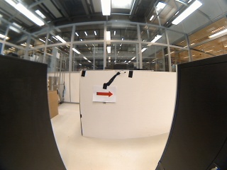
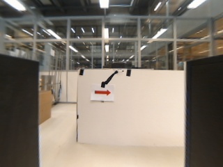
'''Step 1.) Compensate for distortion fish-eye lens''' | |||
<BR> | |||
{| | |||
|- | |||
|[[File:1_InputRosMsg.jpg|thumb|center|300px|Camera image]] | |||
|[[File:2_Undistort.jpg|thumb|center|300px|Undistort image]] | |||
|} | |||
The provided images taken with the camera of Jazz have not a really high quality partially due to the so-called fish-eye effect which causes a distortion. Distorted arrows may be hard to recognize and as the camera properties will most likely not change, we have used to solve this issue by correcting the distortion by a calibration as is described on this webpage: | |||
[http://dasl.mem.drexel.edu/~noahKuntz/openCVTut10.html/ Camera Calibration example] a other webpage is | |||
[http://www.aishack.in/2010/07/calibrating-undistorting-with-opencv-in-c-oh-yeah/ Information on distortion Correction]. | |||
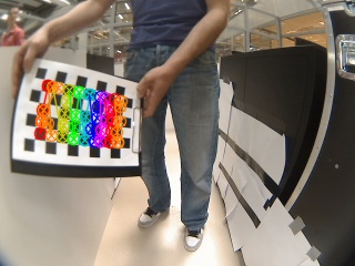
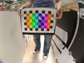
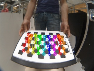
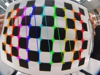
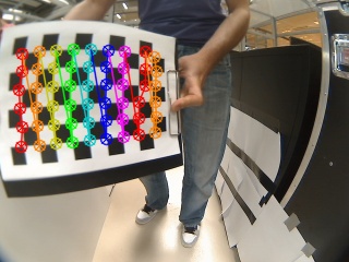
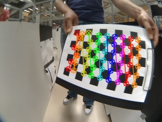
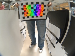
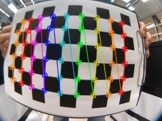
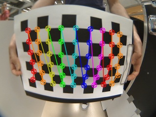
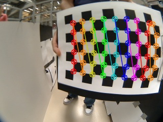
The calibration with the images below is not perfect, because of there were no image captured on the side of the camera. | |||
{| | |||
|- | |||
|[[File:2_Input1.jpg|thumb|center|200px|Calibration image 1]] | |||
|[[File:2_Input2.jpg|thumb|center|200px|Calibration image 2]] | |||
< | |[[File:2_Input3.jpg|thumb|center|200px|Calibration image 3]] | ||
|[[File:2_Input4.jpg|thumb|center|200px|Calibration image 4]] | |||
|- | |||
|[[File:2_Input5.jpg|thumb|center|200px|Calibration image 5]] | |||
<td style="background: | |[[File:2_Input6.jpg|thumb|center|200px|Calibration image 6]] | ||
|[[File:2_Input7.jpg|thumb|center|200px|Calibration image 7]] | |||
|[[File:2_Input8.jpg|thumb|center|200px|Calibration image 8]] | |||
|- | |||
< | |[[File:2_Input9.jpg|thumb|center|200px|Calibration image 9]] | ||
|[[File:2_Input10.jpg|thumb|center|200px|Calibration image 10]] | |||
|[[File:2_Input11.jpg|thumb|center|200px|Calibration image 11]] | |||
|[[File:2_Input12.jpg|thumb|center|200px|Calibration image 12]] | |||
< | |- | ||
|[[File:2_Input13.jpg|thumb|center|200px|Calibration image 13]] | |||
|[[File:2_Input14.jpg|thumb|center|200px|Calibration image 14]] | |||
( | |[[File:2_Input15.jpg|thumb|center|200px|Calibration image 15]] | ||
|} | |||
'''Step 2.) Resize image 2x bigger''' | |||
After lots of testing with our arrow detection algorithm we were still not satisfied with the result. Not because our arrow detection did not work, but because our detection was limited to a small range. Only in less then 1 meter from the arrow we were able to detect the direction of the arrow. The main reason for this is that the resolution of the camera is not so high. Therefore we decided to use linear interpolation to increase the resolution of our input image. We used the function ''Resize''[http://opencv.willowgarage.com/documentation/cpp/imgproc_geometric_image_transformations.html#resize] to increase the resolution in both directions with a factor 2. <br> | |||
We do not get more information with this function, but with a higher resolution we were able to detect more corners. And therefore we got a better determination of the direction of the arrow. | |||
<BR> | |||
{| | |||
|- | |||
|[[File:2_Undistort.jpg|thumb|center|150px|Undistort image]] | |||
|[[File:3_Reszie_2x.jpg|thumb|center|300px|Resized image]] | |||
|} | |||
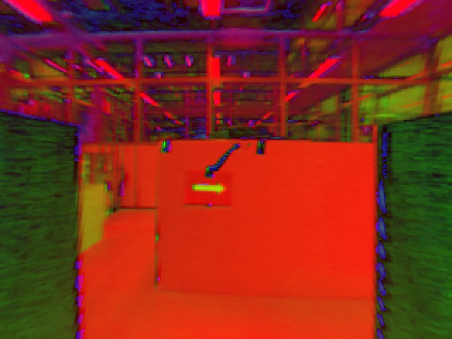
'''Step 3.) Convert image to HSV image''' | |||
<BR> | |||
{| | |||
|- | |||
|[[File:3_Reszie_2x.jpg|thumb|center|300px|Resized image]] | |||
|[[File:4_HSV_image.jpg|thumb|center|300px|HSV image]] | |||
|} | |||
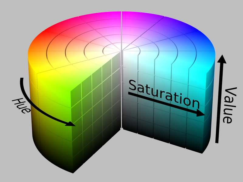
HSV varies the hue component of the hue-saturation-value color model. The colors begin with red, pass through yellow, green, cyan, blue, magenta, and return to red. The advance of using HSV is that you can use a color for different illuminations by using a hue and saturation value. We used is so we are sure that we are looking for a red object. With the saturation and value it is possible to be less sensitive to light. | |||
<center> | |||
[[File:HSV_color_solid_cylinder_alpha_lowgamma.png|400px]] | |||
</center> | |||
<br><br> | |||
<center> | |||
<table style="background-color: rgb(238, 238, 238);"> | |||
<tr> | |||
<td colspan="2"> | |||
<div style="float: right; padding-right: 1em;"> | |||
<div class="noprint plainlinks hlist navbar" style=""> | |||
</div> | |||
</div> | |||
</td> | |||
</tr> | |||
<tr> | |||
<td> | |||
<table style="background-color: rgb(238, 238, 238); padding: 1em;"> | |||
<tr> | |||
<th style="font-weight: normal;"></th> | |||
<th colspan="4" style="font-weight: normal;"><b><i>H</i> = 180°</b><br> | |||
(Cyan)</th> | |||
<th style="font-weight: normal; min-width: 2.2em;"></th> | |||
<th colspan="4" style="font-weight: normal;"><b><i>H</i> = 0°</b><br> | |||
(Red)</th> | |||
</tr> | </tr> | ||
<tr> | <tr> | ||
<th style=" | <th style="min-width: 3em;"><i>V</i> \ <i>S</i></th> | ||
<th style="font-weight: normal; min-width: 2.2em;">1</th> | |||
<th style="font-weight: normal; min-width: 2.2em;">¾</th> | |||
< | |||
< | |||
< | <th style="font-weight: normal; min-width: 2.2em;">½</th> | ||
<th style="font-weight: normal; min-width: 2.2em;">¼</th> | |||
<th style="font-weight: normal; min-width: 2.2em;">0</th> | |||
<th style="font-weight: normal; min-width: 2.2em;">¼</th> | |||
<th style="font-weight: normal; min-width: 2.2em;">½</th> | |||
<th style="font-weight: normal; min-width: 2.2em;">¾</th> | |||
<th style="font-weight: normal; min-width: 2.2em;">1</th> | |||
</tr> | </tr> | ||
<tr> | <tr> | ||
<th style="font-weight: normal;"> | <th style="font-weight: normal;">1</th> | ||
<td style="background: none repeat scroll 0% 0% rgb(0, | |||
G = | <td style="background: none repeat scroll 0% 0% rgb(0, 255, 255);" title="R = 0.000, | ||
B = | G = 1.000, | ||
(# | B = 1.000 | ||
<td style="background: none repeat scroll 0% 0% rgb( | (#00FFFF)"> </td> | ||
G = | <td style="background: none repeat scroll 0% 0% rgb(64, 255, 255);" title="R = 0.250, | ||
B = | G = 1.000, | ||
(# | B = 1.000 | ||
<td style="background: none repeat scroll 0% 0% rgb( | (#40FFFF)"> </td> | ||
G = | <td style="background: none repeat scroll 0% 0% rgb(128, 255, 255);" title="R = 0.500, | ||
B = | G = 1.000, | ||
(# | B = 1.000 | ||
<td style="background: none repeat scroll 0% 0% rgb( | (#80FFFF)"> </td> | ||
G = | <td style="background: none repeat scroll 0% 0% rgb(191, 255, 255);" title="R = 0.750, | ||
B = | G = 1.000, | ||
(# | B = 1.000 | ||
<td style="background: none repeat scroll 0% 0% rgb( | (#BFFFFF)"> </td> | ||
G = | <td style="background: none repeat scroll 0% 0% rgb(255, 255, 255);" title="R = 1.000, | ||
B = | G = 1.000, | ||
(# | B = 1.000 | ||
<td style="background: none repeat scroll 0% 0% rgb( | (#FFFFFF)"> </td> | ||
G = 0. | <td style="background: none repeat scroll 0% 0% rgb(255, 191, 191);" title="R = 1.000, | ||
B = 0. | G = 0.750, | ||
(# | B = 0.750 | ||
<td style="background: none repeat scroll 0% 0% rgb( | (#FFBFBF)"> </td> | ||
G = 0. | <td style="background: none repeat scroll 0% 0% rgb(255, 128, 128);" title="R = 1.000, | ||
B = 0. | G = 0.500, | ||
(# | B = 0.500 | ||
<td style="background: none repeat scroll 0% 0% rgb( | (#FF8080)"> </td> | ||
G = 0. | <td style="background: none repeat scroll 0% 0% rgb(255, 64, 64);" title="R = 1.000, | ||
B = 0. | G = 0.250, | ||
(# | B = 0.250 | ||
<td style="background: none repeat scroll 0% 0% rgb( | (#FF4040)"> </td> | ||
<td style="background: none repeat scroll 0% 0% rgb(255, 0, 0);" title="R = 1.000, | |||
G = 0.000, | G = 0.000, | ||
B = 0.000 | B = 0.000 | ||
(# | (#FF0000)"> </td> | ||
</tr> | </tr> | ||
<tr> | <tr> | ||
<th style="font-weight: normal;"> | <th style="font-weight: normal;">⅞</th> | ||
<td style="background: none repeat scroll 0% 0% rgb(0, 223, 223);" title="R = 0.000, | |||
G = 0.875, | |||
B = 0.875 | |||
(#00DFDF)"> </td> | |||
<td style="background: none repeat scroll 0% 0% rgb(56, 223, 223);" title="R = 0.219, | |||
G = 0.875, | |||
B = 0.875 | |||
(#38DFDF)"> </td> | |||
<td style="background: none repeat scroll 0% 0% rgb(112, 223, 223);" title="R = 0.438, | |||
G = 0.875, | |||
B = 0.875 | |||
(#70DFDF)"> </td> | |||
<td style="background: none repeat scroll 0% 0% rgb(167, 223, 223);" title="R = 0.656, | |||
G = 0.875, | |||
B = 0.875 | |||
(#A7DFDF)"> </td> | |||
<td style="background: none repeat scroll 0% 0% rgb(0, | <td style="background: none repeat scroll 0% 0% rgb(223, 223, 223);" title="R = 0.875, | ||
G = 0. | G = 0.875, | ||
B = 0. | B = 0.875 | ||
(# | (#DFDFDF)"> </td> | ||
<td style="background: none repeat scroll 0% 0% rgb( | <td style="background: none repeat scroll 0% 0% rgb(223, 167, 167);" title="R = 0.875, | ||
G = 0. | G = 0.656, | ||
B = 0. | B = 0.656 | ||
(# | (#DFA7A7)"> </td> | ||
<td style="background: none repeat scroll 0% 0% rgb( | <td style="background: none repeat scroll 0% 0% rgb(223, 112, 112);" title="R = 0.875, | ||
G = 0. | G = 0.438, | ||
B = 0. | B = 0.438 | ||
(# | (#DF7070)"> </td> | ||
<td style="background: none repeat scroll 0% 0% rgb(96, | <td style="background: none repeat scroll 0% 0% rgb(223, 56, 56);" title="R = 0.875, | ||
G = 0. | G = 0.219, | ||
B = 0. | B = 0.219 | ||
(# | (#DF3838)"> </td> | ||
<td style="background: none repeat scroll 0% 0% rgb( | <td style="background: none repeat scroll 0% 0% rgb(223, 0, 0);" title="R = 0.875, | ||
G = 0. | G = 0.000, | ||
B = 0. | B = 0.000 | ||
(# | (#DF0000)"> </td> | ||
<td style="background: none repeat scroll 0% 0% rgb( | </tr> | ||
G = 0.375, | <tr> | ||
<th style="font-weight: normal;">¾</th> | |||
<td style="background: none repeat scroll 0% 0% rgb(0, 191, 191);" title="R = 0.000, | |||
G = 0.750, | |||
B = 0.750 | |||
(#00BFBF)"> </td> | |||
<td style="background: none repeat scroll 0% 0% rgb(48, 191, 191);" title="R = 0.188, | |||
G = 0.750, | |||
B = 0.750 | |||
(#30BFBF)"> </td> | |||
<td style="background: none repeat scroll 0% 0% rgb(96, 191, 191);" title="R = 0.375, | |||
G = 0.750, | |||
B = 0.750 | |||
(#60BFBF)"> </td> | |||
<td style="background: none repeat scroll 0% 0% rgb(143, 191, 191);" title="R = 0.562, | |||
G = 0.750, | |||
B = 0.750 | |||
(#8FBFBF)"> </td> | |||
<td style="background: none repeat scroll 0% 0% rgb(191, 191, 191);" title="R = 0.750, | |||
G = 0.750, | |||
B = 0.750 | |||
(#BFBFBF)"> </td> | |||
<td style="background: none repeat scroll 0% 0% rgb(191, 143, 143);" title="R = 0.750, | |||
G = 0.562, | |||
B = 0.562 | |||
(#BF8F8F)"> </td> | |||
<td style="background: none repeat scroll 0% 0% rgb(191, 96, 96);" title="R = 0.750, | |||
G = 0.375, | |||
B = 0.375 | B = 0.375 | ||
(# | (#BF6060)"> </td> | ||
<td style="background: none repeat scroll 0% 0% rgb( | <td style="background: none repeat scroll 0% 0% rgb(191, 48, 48);" title="R = 0.750, | ||
G = 0. | G = 0.188, | ||
B = 0. | B = 0.188 | ||
(# | (#BF3030)"> </td> | ||
<td style="background: none repeat scroll 0% 0% rgb(191, 0, 0);" title="R = 0.750, | |||
<td style="background: none repeat scroll 0% 0% rgb( | |||
G = 0.000, | G = 0.000, | ||
B = 0.000 | B = 0.000 | ||
(# | (#BF0000)"> </td> | ||
</tr> | </tr> | ||
<tr> | <tr> | ||
<th style="font-weight: normal;"> | <th style="font-weight: normal;">⅝</th> | ||
<td style="background: none repeat scroll 0% 0% rgb(0, | <td style="background: none repeat scroll 0% 0% rgb(0, 159, 159);" title="R = 0.000, | ||
G = 0. | G = 0.625, | ||
B = 0. | B = 0.625 | ||
(# | (#009F9F)"> </td> | ||
<td style="background: none repeat scroll 0% 0% rgb( | <td style="background: none repeat scroll 0% 0% rgb(40, 159, 159);" title="R = 0.156, | ||
G = 0. | G = 0.625, | ||
B = 0. | B = 0.625 | ||
(# | (#289F9F)"> </td> | ||
<td style="background: none repeat scroll 0% 0% rgb( | <td style="background: none repeat scroll 0% 0% rgb(80, 159, 159);" title="R = 0.312, | ||
G = 0. | G = 0.625, | ||
B = 0. | B = 0.625 | ||
(# | (#509F9F)"> </td> | ||
<td style="background: none repeat scroll 0% 0% rgb( | <td style="background: none repeat scroll 0% 0% rgb(120, 159, 159);" title="R = 0.469, | ||
G = 0. | G = 0.625, | ||
B = 0. | B = 0.625 | ||
(# | (#789F9F)"> </td> | ||
<td style="background: none repeat scroll 0% 0% rgb(159, 159, 159);" title="R = 0.625, | |||
G = 0.625, | |||
B = 0.625 | |||
(#9F9F9F)"> </td> | |||
<td style="background: none repeat scroll 0% 0% rgb(159, 120, 120);" title="R = 0.625, | |||
G = 0.469, | |||
B = 0.469 | |||
(#9F7878)"> </td> | |||
<td style="background: none repeat scroll 0% 0% rgb(159, 80, 80);" title="R = 0.625, | |||
G = 0.312, | |||
B = 0.312 | |||
(#9F5050)"> </td> | |||
<td style="background: none repeat scroll 0% 0% rgb(159, 40, 40);" title="R = 0.625, | |||
G = 0.156, | |||
B = 0.156 | |||
(#9F2828)"> </td> | |||
<td style="background: none repeat scroll 0% 0% rgb(159, 0, 0);" title="R = 0.625, | |||
G = 0.000, | |||
B = 0.000 | |||
(#9F0000)"> </td> | |||
</tr> | |||
<tr> | |||
<th style="font-weight: normal;">½</th> | |||
<td style="background: none repeat scroll 0% 0% rgb(96, 96, 96);" title="R = 0. | <td style="background: none repeat scroll 0% 0% rgb(0, 128, 128);" title="R = 0.000, | ||
G = 0.500, | |||
B = 0.500 | |||
(#008080)"> </td> | |||
<td style="background: none repeat scroll 0% 0% rgb(32, 128, 128);" title="R = 0.125, | |||
G = 0.500, | |||
B = 0.500 | |||
(#208080)"> </td> | |||
<td style="background: none repeat scroll 0% 0% rgb(64, 128, 128);" title="R = 0.250, | |||
G = 0.500, | |||
B = 0.500 | |||
(#408080)"> </td> | |||
<td style="background: none repeat scroll 0% 0% rgb(96, 128, 128);" title="R = 0.375, | |||
G = 0.500, | |||
B = 0.500 | |||
(#608080)"> </td> | |||
<td style="background: none repeat scroll 0% 0% rgb(128, 128, 128);" title="R = 0.500, | |||
G = 0.500, | |||
B = 0.500 | |||
(#808080)"> </td> | |||
<td style="background: none repeat scroll 0% 0% rgb(128, 96, 96);" title="R = 0.500, | |||
G = 0.375, | G = 0.375, | ||
B = 0.375 | B = 0.375 | ||
(# | (#806060)"> </td> | ||
<td style="background: none repeat scroll 0% 0% rgb( | <td style="background: none repeat scroll 0% 0% rgb(128, 64, 64);" title="R = 0.500, | ||
G = 0. | G = 0.250, | ||
B = 0. | B = 0.250 | ||
(# | (#804040)"> </td> | ||
<td style="background: none repeat scroll 0% 0% rgb( | <td style="background: none repeat scroll 0% 0% rgb(128, 32, 32);" title="R = 0.500, | ||
G = 0. | G = 0.125, | ||
B = 0. | B = 0.125 | ||
(# | (#802020)"> </td> | ||
<td style="background: none repeat scroll 0% 0% rgb( | <td style="background: none repeat scroll 0% 0% rgb(128, 0, 0);" title="R = 0.500, | ||
G = 0.000, | G = 0.000, | ||
B = 0.000 | B = 0.000 | ||
(# | (#800000)"> </td> | ||
</tr> | </tr> | ||
<tr> | <tr> | ||
<th style="font-weight: normal;"> | <th style="font-weight: normal;">⅜</th> | ||
<td style="background: none repeat scroll 0% 0% rgb(0, | <td style="background: none repeat scroll 0% 0% rgb(0, 96, 96);" title="R = 0.000, | ||
G = 0. | G = 0.375, | ||
B = 0. | B = 0.375 | ||
(# | (#006060)"> </td> | ||
<td style="background: none repeat scroll 0% 0% rgb( | <td style="background: none repeat scroll 0% 0% rgb(24, 96, 96);" title="R = 0.094, | ||
G = 0. | G = 0.375, | ||
B = 0. | B = 0.375 | ||
(# | (#186060)"> </td> | ||
<td style="background: none repeat scroll 0% 0% rgb( | <td style="background: none repeat scroll 0% 0% rgb(48, 96, 96);" title="R = 0.188, | ||
G = 0. | G = 0.375, | ||
B = 0. | B = 0.375 | ||
(# | (#306060)"> </td> | ||
<td style="background: none repeat scroll 0% 0% rgb( | <td style="background: none repeat scroll 0% 0% rgb(72, 96, 96);" title="R = 0.281, | ||
G = 0. | G = 0.375, | ||
B = 0. | B = 0.375 | ||
(# | (#486060)"> </td> | ||
<td style="background: none repeat scroll 0% 0% rgb( | |||
G = 0. | <td style="background: none repeat scroll 0% 0% rgb(96, 96, 96);" title="R = 0.375, | ||
B = 0. | G = 0.375, | ||
(# | B = 0.375 | ||
<td style="background: none repeat scroll 0% 0% rgb( | (#606060)"> </td> | ||
<td style="background: none repeat scroll 0% 0% rgb(96, 72, 72);" title="R = 0.375, | |||
G = 0.281, | |||
B = 0.281 | |||
(#604848)"> </td> | |||
<td style="background: none repeat scroll 0% 0% rgb(96, 48, 48);" title="R = 0.375, | |||
G = 0.188, | G = 0.188, | ||
B = 0.188 | B = 0.188 | ||
(#403030)"> </td> | (#603030)"> </td> | ||
<td style="background: none repeat scroll 0% 0% rgb(96, 24, 24);" title="R = 0.375, | |||
G = 0.094, | |||
B = 0.094 | |||
(#601818)"> </td> | |||
<td style="background: none repeat scroll 0% 0% rgb(96, 0, 0);" title="R = 0.375, | |||
G = 0.000, | |||
B = 0.000 | |||
(#600000)"> </td> | |||
</tr> | |||
<tr> | |||
<th style="font-weight: normal;">¼</th> | |||
<td style="background: none repeat scroll 0% 0% rgb(0, 64, 64);" title="R = 0.000, | |||
G = 0.250, | |||
B = 0.250 | |||
(#004040)"> </td> | |||
<td style="background: none repeat scroll 0% 0% rgb(16, 64, 64);" title="R = 0.062, | |||
G = 0.250, | |||
B = 0.250 | |||
(#104040)"> </td> | |||
<td style="background: none repeat scroll 0% 0% rgb(32, 64, 64);" title="R = 0.125, | |||
G = 0.250, | |||
B = 0.250 | |||
(#204040)"> </td> | |||
<td style="background: none repeat scroll 0% 0% rgb(48, 64, 64);" title="R = 0.188, | |||
G = 0.250, | |||
B = 0.250 | |||
(#304040)"> </td> | |||
<td style="background: none repeat scroll 0% 0% rgb(64, 64, 64);" title="R = 0.250, | |||
G = 0.250, | |||
B = 0.250 | |||
(#404040)"> </td> | |||
<td style="background: none repeat scroll 0% 0% rgb(64, 48, 48);" title="R = 0.250, | |||
G = 0.188, | |||
B = 0.188 | |||
(#403030)"> </td> | |||
<td style="background: none repeat scroll 0% 0% rgb(64, 32, 32);" title="R = 0.250, | <td style="background: none repeat scroll 0% 0% rgb(64, 32, 32);" title="R = 0.250, | ||
G = 0.125, | G = 0.125, | ||
| Line 2,465: | Line 2,577: | ||
<br><br> | <br><br> | ||
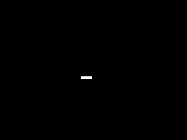
'''Step 4.) Convert red pixels to black and white image''' | |||
<BR> | |||
{| | |||
|- | |||
|[[File:4_HSV_image.jpg|thumb|center|300px|HSV image]] | |||
|[[File:5_Binary_Image.jpg|thumb|center|300px|Blck white image out of the red]] | |||
|} | |||
From the HSV image we create a black and white image. In the tables above you can | From the HSV image we create a black and white image (binary image). In the tables above you can see which values to use if you only want to find red arrows. We implemented a track-bar for each parameter to find easily the ideal parameters settings for a variety of conditions. This resulted in the following boundaries for each parameter: | ||
<center> | <center> | ||
<math> | <math> | ||
(H \leq | (H \leq 16 \vee H \geq 343) \land S \geq 0.50 \land V \geq 0.50 | ||
</math> | </math> | ||
<br><br> | <br><br> | ||
| Line 2,478: | Line 2,596: | ||
<br> | <br> | ||
'''Step 5.) Find biggest contour''' | |||
Afther the conversion of the HSV image to a binary image there was still some noise in our image. Probably as a result of reflection of the light and the presence of other red objects near the red arrow. Therefore we search in the binary image for closed contours, i.e. for object pixels that are connected with each other, using the ''FindContours''[http://opencv.willowgarage.com/documentation/c/imgproc_structural_analysis_and_shape_descriptors.html#findcontours] function of OpenCV. For each contours we calculate the area and store the biggest contour. We use a threshold value (a minimum area) the biggest object must have to proceed with the algorithm. Since from a far distance the shape of an arrow is not clearly visible. This is also prevented by only calling the Arrow algorithm at a short distance from a t-junction. Since only the biggest contour remains the residual noise is filtered out and only a possible arrow is left. | |||
<BR> | |||
{| | |||
< | |- | ||
|[[File:5_Binary_Image.jpg|thumb|center|300px|Black white image out of the red]] | |||
|[[File:6_Biggest_contour.jpg|thumb|center|300px|Biggest_contour]] | |||
|} | |||
'''Step 6.) Region of interest''' | |||
<BR> | |||
{| | |||
|- | |||
|[[File:5_Binary_Image.jpg|thumb|center|300px|Black white image out of the red]] | |||
|[[File:6_Biggest_contour.jpg|thumb|center|300px|Biggest_contour]] | |||
|} | |||
Region of Interest is a rectangular area in an image, to segment object for further processing. The ilustration is shown in Figure 1 below. For speeding up the algorithm we take 50 pixel up, down, left and right bigger as the boundaries of the contour. So that the watershed segmentation cannot segment something what is not red or not interested in. | |||
[[File:ROI.gif|thumb|center|400px|Figure 1 Region of Interest]] | |||
'''Step 7.) Watershed segmentation''' | |||
<BR> | |||
{| | |||
|- | |||
|[[File:6_Biggest_contour.jpg|thumb|center|500px|Biggest_contour]] | |||
|[[File:10_WaterShed_Bw.jpg|thumb|center|500px|Watershed Black and White image]] | |||
|[[File:9_WaterShed_Color.jpg|thumb|center|500px|Watershed color image]] | |||
|} | |||
We have used the watershed segmentation so we get a all the information of the arrow possible out of the image at a bigger distance. | |||
The are different approaches may be employed to use the watershed principle for image segmentation. | |||
* Local minima of the gradient of the image may be chosen as markers, in this case an over-segmentation is produced and a second step involves region merging. | |||
* Marker based watershed transformation make use of specific marker positions which have been either explicitly defined by the user or determined automatically with morphological operators or other ways. | |||
We have used the Marker based watershed transformation. | |||
<br> | '''Step 8.) Match the shape of the contour with a template arrow''' | ||
If a contour is found does this not directly mean that it is also a arrow. Therefore the function ''MatchShapes''[http://opencv.willowgarage.com/documentation/cpp/imgproc_structural_analysis_and_shape_descriptors.html#matchShapes] is used to compare the shape of the contour with a predefined template arrow. This function calculates the rotation invariant moments[http://en.wikipedia.org/wiki/Image_moment#Rotation_invariant_moments] (Hu moments) of each possible arrow that we get. Then the function compares the Hu moments with the Hu moments of a template arrow which we recorded earlier. And compares these two sets of Hu moments and gives a result in the form of a certain value. The lower the value (ideally is 0) the more similarities between the two Hu moments and thus the more simularities between the two shapes. A lot of testing is done to find an reliable maximum value.<br>The advantage of the Hu moments is that they are invariant under translation, changes in scale, and also rotation. So this ''MatchShapes'' function will also work properly with slightly rotated arrows or when the detected arrow is of a different size than the template arrow. Or even when the arrow points to the other direction then our template arrow. | |||
'''Step 9.) Corner detection''' | |||
< | To detect the direction of the arrow we use the function ''Cornersubpix''[http://opencv.willowgarage.com/documentation/cpp/imgproc_feature_detection.html?highlight=corner#cornerSubPix] to calculate the corners of the arrow. Based on this corners we determine the direction of the arrow, by looking at which side the most corners are found. Because the resolution of the arrow is still not perfect, the function ''Cornersubpix'' sometimes detects corners along the edge in the middle of the arrow. Which also can be seen in the picture below. Therefore we implemented a filter which filters out the corners which are detected within a certain area around the centre point of the arrow. With the result that only the actual corners of the arrow are left, resulting in a correct detection of the direction of the arrow. | ||
<BR> | |||
{| | |||
|- | |||
|[[File:10_WaterShed_Bw.jpg|thumb|center|200px|Watershed Black and White image]] | |||
|[[File:11_corners.jpg|thumb|center|200px|Corners of the arrow]] | |||
|} | |||
=== | ===Overview process=== | ||
{| | |||
|- | |||
|[[File:1_InputRosMsg.jpg|thumb|center|150px|Original image]] | |||
|[[File:2_Undistort.jpg|thumb|center|150px|Undistort]] | |||
|[[File:3_Reszie_2x.jpg|thumb|center|200px|Resize 2x]] | |||
|[[File:4_HSV_image.jpg|thumb|center|200px|HSV image]] | |||
|- | |||
||[[File:5_Binary_Image.jpg|thumb|center|200px|Binary]] | |||
|[[File:6_Biggest_contour.jpg|thumb|center|200px|Biggest contour and ROI]] | |||
|[[File:10_WaterShed_Bw.jpg|thumb|center|200px|Watershed segmentetion]] | |||
|[[File:11_corners.jpg|thumb|center|200px|Corner detection]] | |||
|} | |||
==== | ===Video of testing arrow algorithm=== | ||
We have recorded two video's while running the arrow detection algorithm. The first one was the first test with a bag file. Not al the functions we discussed above were implemented yet during this test. The second one is our final test. With a driving Jazz robot controlled by the remote control. | |||
<center><span style="padding: 5px; clear:both; margin:15px; width: 500px;">[[File:Arrow_detection_test.png|350px|Test video of arrow detection|link=http://www.youtube.com/watch?v=boLSpT61_q0&feature=g-upl]]</span></center><br> | |||
<br> | |||
<center><span style="padding: 5px; clear:both; margin:15px; width: 500px;">[[File:Arrow_detection.png|350px|link=http://www.youtube.com/watch?v=3s5daBhY9uQ&feature=youtu.be|Video of final test with the arrow detection algorithm]]</span></center><br> | |||
== | ==Overall algorithm== | ||
=== | ===Driving fases=== | ||
<br> | |||
'''Initialisation fase'''<br> | |||
This fase only runs in the beginning and in some failsafe cases (see below). During this fase Jazz finds the line that is closest and turns untill its heading direction is parallel to this line. The initialisation fase then ends and the parallel driving fase starts. | |||
<br><br> | |||
'''Parallel driving fase'''<br> | |||
In this fase Jazz tries to move parallel to the closest parallel line. This is achieved by controlling the radspeed dependent of the difference in angle between the driving direction and the parallel line (shown below). If Jazz is not in the safe zone an offset is given to this angle to move towards the safe zone. The forward velocity is also dependent of the zone where Jazz is in. | |||
<center> | <center> | ||
[[ | [[File:Paralleldriving.png|thumb|none|300px]] | ||
</center> | |||
<br><br> | |||
'''Turning fase'''<br> | |||
In this fase Jazz turns left or right. The turning fase has two subfases, in the first fase Jazz does not start turning yet but moves towards the exitline (shown in the picture below) untill the distance to this exitline is half the hallwidth. Then the forward velocity is set to zero and Jazz begins turning, this is done by controlling the radspeed bependent of the difference in angle between the driving direction and the exitline. The angle with this exitline is monitored and if it is close to parallel the turning fase ends and the parallel driving fase starts. | |||
<center> | <center> | ||
[[ | {| | ||
</center><br><br> | |[[File:Turning1.png|thumb|none|300px]] | ||
The | |[[File:Turning2.png|thumb|none|300px]] | ||
|} | |||
</center> | |||
<br><br> | |||
'''Dead end fase'''<br> | |||
In this fase Jazz turns 180 degrees drives back into the corridor where it came from. The forward velocity is set to zero and Jazz starts turning untill it is parallel in the corridor again. How this works is shown in the picture below. | |||
<center> | <center> | ||
[[ | [[File:Deadend.png|thumb|none|300px]] | ||
</center> | </center> | ||
<br><br> | <br><br> | ||
===Exit detection=== | |||
The exit detection searches for lines that are at an angle of approximately 90 degrees. If a line like this is found the type of junction is determined and if this is done the exit handling starts. The exit detection is then suspended untill Jazz has moved out of the current junction. This is done by monitoring a line that cannot be detected anymore when Jazz has moved out of the junction, so when this line cannot be monitored any more the exit detection is not suspended anymore. Which line this is is shown in the picture below. | |||
<center> | <center> | ||
[[ | [[File:Exitdetectionend.png|thumb|none|300px]] | ||
</center> | </center> | ||
<br><br> | <br><br> | ||
The | ===Arrow detection=== | ||
The arrow detection is only called when a T-junction is detected, because this is the only place where the arrows could be placed. The arrow detection service then returns a value 0, 1 or 2. 0 means there is no arrow detected, 1 is for a left arrow, 2 for a right arrow. How this arrow is used is explained in the exit handling below. | |||
The | <br><br> | ||
===Exit handling=== | |||
The exit handling is executed when an exit is detected. It receives data that contains information about where the exits are and how many times they have been visited before and the arrow direction. The exit handling decides which exit to take by using Tremaux's algorithm, so it picks the exit with the least amounts of visits. When the exits have the same amount of visits the exit normally should be picked randomly according to Tremaux's algorithm. However we have chosen that if there is a front exit, this exit should be preferred because turning takes more time. If there is no front exit or this exit has more visits, left and right are picked randomly. | |||
An exception is made for when an arrow is detected, the direction of the arrow is then preferred. When the direction of the arrow has more visits than one of the other exits, the arrow is ignored. This is to ensure that the maze will be solved, even when an arrow is detected wrong. | |||
=== | ===Fail-safes=== | ||
To | To prevent deadlocks or collisions some fail-safes are introduced. | ||
# Laserdata age: If the received laserdata is older then 500ms Jazz stops moving and waits for new laserdata. | |||
# Monitored lines are not found: If lines that are monitored and disappear when they are not expected to (this is during the turning or dead end fase), Jazz stops moving for 1 second. If the line is not found within this second Jazz goes back to the parallel driving fase. | |||
# No parallel lines are found: If during the parallel driving fase no parallel lines are found, Jazz stops moving. If there are no parallel lines found within a second Jazz goes back to the initialisation fase. | |||
# No lines detected: If there are no lines detected at all, Jazz stops moving. If no lines are detected within 5 seconds Jazz slowly starts rotating untill one or more lines are detected. | |||
# Arrow detection service fails: If the arrow detection service fails or is not running Jazz can still function by using only Tremaux's algorithm. | |||
# Dump Map service fails: If the map service fails or is not running Jazz can still function by switching to the wallfollower algorithm. | |||
<br><br> | |||
=== | ==Simulation versus real world== | ||
===Temporarily solution for the laserdata points=== | |||
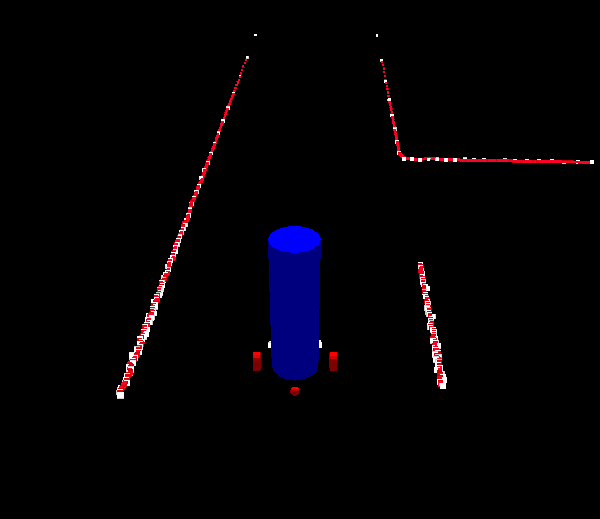
Because we encountered some unexpected problems during the first test on the real robot we have made some modification to the simulator so it becomes a better representation of the real world. Our line detection uses the laserdata as an input and was optimized for the laserscanner of the simulator which returned 180 points. The real laserscanner returns 1080 points, which our program could not handle. To prevent this problem in the future an extra program is written that takes in the 180 points laserdata from the simulator and transforms this to 1080 points laserdata. This is done by lineair interpolation between the points of the simulated laserdata. | |||
The visualisation of the new laserdata is shown in de picture below, the red dots represent the points from the new simulated laserdata, the white dots are those from the old simulated laserdata. | |||
<br><br> | |||
<center> | <center> | ||
[[Image: | [[Image:Oldvsnewlaserdata.png |400px]] | ||
</center> | </center><br><br> | ||
===Walls=== | |||
We also made a corridor in the simulator that does not have perfectly straight walls, because in reality this is also not the case. For testing the robustness of our line detection algorithm this is very useful. The difference between the old and new corridor world is shown below. | |||
<br><br> | |||
<center> | |||
[[Image:Corridorold.png |600px]]<br> | |||
Original corridor world with perfectly straight walls. | |||
</center><br> | |||
<center> | |||
[[Image:Corridornew.png |600px]]<br> | |||
Modified corridor world with walls that are not perfectly straight. | |||
</center><br><br> | |||
===Synchronisation issues=== | |||
To make sure our algorithm worked properly some messages had to be synchronized, this all went well in the simulator. In the real world test the messages would not synchronize in some cases, this was caused by the fact that the program ran on an external workstation. Both the workstation and Jazz have their own system time and some messages received their time stamp from Jazz' system time and others from the workstation's system time. These messages can not by synchronized properly. We decided to take out the synchronization and during the tests this went well, but this is no guarantee that it will never cause problems. | |||
<br><br> | |||
===Communication delays=== | |||
Because the control of Jazz is executed on an external workstation Jazz suffered from communication delay. Because of this delay we decided to increase the critical zone of the corridor and tune down some parameters which resulted in a slower moving Jazz. This was the only way to make Jazz stable. In the final competition our Jazz moved very slowly but also was the only one which made it through the maze. With some more test time we would be able to make it a bit faster, but the delays in communication were the most limiting factor.<br><br> | |||
==Presentation Final competition June 29th 2012== | |||
[http://cstwiki.wtb.tue.nl/images/Final_presentation_7.pdf Final Presentation] | |||
== | ==Jazz's Blog== | ||
== | <p>In this section I will publish all kinds of information on the things I am currently learning, I have learned so far and my further ambitions.</p> | ||
<div style="background-color: #D8D8D8; border: 1px solid #000; width: 600px; margin-left:15px; margin-bottom: 30px; -moz-border-radius: 15px; border-radius: 15px; background: -moz-linear-gradient(top, #1919FF, #BABAFF);background: -webkit-gradient(linear, left top, left bottom, from(#1919FF), to(#BABAFF)); text-align: justify;" > | |||
<br>< | <h3 style="margin-left: 15px; text-shadow: #6374AB 2px 2px 1px;">29th of June 2012 – I won the final contest!</h3> | ||
< | <p style="margin-left: 15px; margin-right: 15px;"><br>It was an awesome day today. I was able to complete the final contest within the fastest time. Not everything went perfect because some parameters of my program were not optimized due to limited test time, nevertheless I have made me and my bosses very proud. Look at the video below to see me driving through the maze.<br> | ||
[[ | <center><span style="padding: 5px; clear:both; margin:15px; width: 500px;">[[File:Finalcontestvid.png|350px|link=http://www.youtube.com/watch?v=AZCknUOIADc]]</span></center><br></p> | ||
</center><br>< | </div> | ||
=== | |||
<br>< | <div style="background-color: #D8D8D8; border: 1px solid #000; width: 600px; margin-left:15px; margin-bottom: 30px; -moz-border-radius: 15px; border-radius: 15px; background: -moz-linear-gradient(top, #1919FF, #BABAFF);background: -webkit-gradient(linear, left top, left bottom, from(#1919FF), to(#BABAFF)); text-align: justify;" > | ||
< | <h3 style="margin-left: 15px; text-shadow: #6374AB 2px 2px 1px;">27th of June 2012 – Final tests</h3> | ||
[[ | <p style="margin-left: 15px; margin-right: 15px;"><br>Today, I had my last oppertunity to test in a real maze, and as last Thursday my communication suffered again from delays up to a 4 seconds, even by calling just "pico ping". But after reporting this situation someone passed by who fixed this issue of netwrok overload, and afterwards, my tests went pretty well as I can drive through the maze completely autonomously while making a map and looking up how many times an exit is visited at a junction. The arrow recognition is not robust enough yet, but I have some ideas on how to improve robustness for the final competition! Will be continued...<br></p> | ||
</div> | |||
</center><br> | |||
< | |||
<div style="background-color: #D8D8D8; border: 1px solid #000; width: 600px; margin-left:15px; margin-bottom: 30px; -moz-border-radius: 15px; border-radius: 15px; background: -moz-linear-gradient(top, #1919FF, #BABAFF);background: -webkit-gradient(linear, left top, left bottom, from(#1919FF), to(#BABAFF)); text-align: justify;" > | |||
<h3 style="margin-left: 15px; text-shadow: #6374AB 2px 2px 1px;">26th of June 2012 – Achieved one of my ultimate goals!</h3> | |||
< | <p style="margin-left: 15px; margin-right: 15px;"><br>It was a great day today, as I succeeded to solve several maze's in simulation using Tremaux's algorithm, with different types of junction handling in case of an equal number of visits of several directions at a junction. A video is shown below and I hope to achieve this also in the experiments. So, hope to have more good news later...<br> | ||
<center><span style="padding: 5px; clear:both; margin:15px; width: 500px;">[[File:Tremauxvid.png|350px|link=http://www.youtube.com/watch?v=Gp3PYlrQg_s]]</span></center><br></p> | |||
</div> | |||
<div style="background-color: #D8D8D8; border: 1px solid #000; width: 600px; margin-left:15px; margin-bottom: 30px; -moz-border-radius: 15px; border-radius: 15px; background: -moz-linear-gradient(top, #1919FF, #BABAFF);background: -webkit-gradient(linear, left top, left bottom, from(#1919FF), to(#BABAFF)); text-align: justify;" > | |||
<h3 style="margin-left: 15px; text-shadow: #6374AB 2px 2px 1px;">21th of June 2012 – Real world test 3</h3> | |||
<p style="margin-left: 15px; margin-right: 15px;"><br>Today, I had my third test event, but that was not a big succes. The communication between me and the computer suffered from HUGE delays up to 10 seconds and more. Sometimes the communcation broke down completely. However, once the communcation was up and running properly the test were a succes, except for a missing transform needed to test the mapping algorithm implemented to perform the Tremaux's Algorithm. This issue is solved yet so I hope to show you some evidence in the coming few hours or days.<br></p> | |||
</div> | |||
<div style="background-color: #D8D8D8; border: 1px solid #000; width: 600px; margin-left:15px; margin-bottom: 30px; -moz-border-radius: 15px; border-radius: 15px; background: -moz-linear-gradient(top, #1919FF, #BABAFF);background: -webkit-gradient(linear, left top, left bottom, from(#1919FF), to(#BABAFF)); text-align: justify;" > | <div style="background-color: #D8D8D8; border: 1px solid #000; width: 600px; margin-left:15px; margin-bottom: 30px; -moz-border-radius: 15px; border-radius: 15px; background: -moz-linear-gradient(top, #1919FF, #BABAFF);background: -webkit-gradient(linear, left top, left bottom, from(#1919FF), to(#BABAFF)); text-align: justify;" > | ||
| Line 2,631: | Line 2,806: | ||
<div style="background-color: #D8D8D8; border: 1px solid #000; width: 600px; margin-left:15px; margin-bottom: 30px; -moz-border-radius: 15px; border-radius: 15px; background: -moz-linear-gradient(top, #1919FF, #BABAFF);background: -webkit-gradient(linear, left top, left bottom, from(#1919FF), to(#BABAFF)); text-align: justify;" > | <div style="background-color: #D8D8D8; border: 1px solid #000; width: 600px; margin-left:15px; margin-bottom: 30px; -moz-border-radius: 15px; border-radius: 15px; background: -moz-linear-gradient(top, #1919FF, #BABAFF);background: -webkit-gradient(linear, left top, left bottom, from(#1919FF), to(#BABAFF)); text-align: justify;" > | ||
<h3 style="margin-left: 15px; text-shadow: #6374AB 2px 2px 1px;">5th of June 2012 – Recognition of the junction types</h3> | <h3 style="margin-left: 15px; text-shadow: #6374AB 2px 2px 1px;">5th of June 2012 – Recognition of the junction types</h3> | ||
<p style="margin-left: 15px; margin-right: 15px;"><br>Today, I have learned to recognize the different types of junctions described in the section junction handling. I have only to pay some more attention to see at which side the corner (junction type A) is directed and at which side the exit is in case of junction type E. Will be continued soon...<br><br>In the meanwhile, I have also overcome the challenge of detecting the side of the exit for junction type A and E. Now, I only have to recognize arrows and look at the map to take appropriate actions according to Tremaux's Algorithm<br></p> | <p style="margin-left: 15px; margin-right: 15px;"><br>Today, I have learned to recognize the different types of junctions described in the section junction handling. I have only to pay some more attention to see at which side the corner (junction type A) is directed and at which side the exit is in case of junction type E. Will be continued soon...<br><br>In the meanwhile, I have also overcome the challenge of detecting the side of the exit for junction type A and E. Now, I only have to recognize arrows and look at the map to take appropriate actions according to Tremaux's Algorithm. See the video below of how I am detecting the junction types.<br><center><span style="padding: 5px; clear:both; margin:15px; width: 500px;">[[File:Exittypesvid.png|350px|link=http://www.youtube.com/watch?v=XsCXJzovzT4]]</span></center></p> | ||
</div> | </div> | ||
Latest revision as of 05:01, 2 July 2012
Group Info
| Group Members - | email (at student.tue.nl) |
| Siddhi Imming | s.imming |
| Bart Moris | b.moris |
| Roger Pouls | r.c.e.pouls |
| Patrick Vaes | p.r.m.p.vaes |
Tutor
Rob Janssen - R dot J dot M dot Janssen at tue dot nl
Planning
| General | Weekly meetings with group on Tuesday, Wednesday and Thursday. At least a weekly update of the wiki. Tasks are divided weekly. | ||
| Week 3 (7 may) | Write code to create a 2D map from the laser data. Write code for position control. Read chapter 9 from the book. | ||
| Navigation team | Image processing team | ||
| Week 4 (14 may) | Recognize the direction of walls Recognize opening in walls | Install webcam in ROS gscam. Get familiar with openCV for image processing. | |
| Week 5 (21 may) | Write code for the navigation for the corridor competition. Make sure the Jazz recognizes exits. Prepare the lecture. | Make algorithm in MATLAB on example images. Prepare lecture. | |
| Week 6 (28 may) | Give the lecture. Finish and test the navigation for the corridor competition. Make sure Jazz takes the first exit. | Implement MATLAB algorithm in ROS with openCV. | |
| Week 7 (4 jun) | Corridor competition. Write code for image recognition. Make sure arrows and their pointing direction are recognized. Discuss and choose a strategy for solving the maze. Start implementing the strategy into the navigation code. | Test algorithm with the Jazz Robot. Make images with Jazz Robot and test in MATLAB. Improve algorithm and test on Jazz Robot. | |
| Week 8 (11 jun) | Continue implementing the strategy into the navigation code. | ||
| Week 9 (18 jun) | Finish implementing the strategy into the navigation code. | ||
| Week 10/11 (25 jun / 2 jul) | Final competition. | ||
Goals
Our main goal is to be able to solve the maze Jazz we will be faced with during the final competition. As the philosophy in the world of robotics and also behind the ROS platform is to share knowledge and to use knowledge of others in order to speed up the design process. Of course, we take care of not just plugging in some code designed by others without really understanding what is going on and on what principles the process is based on. So our focus will be on designing a robust and fast navigation algorithm, rather than designing all kinds of new implementations of really nice functions that are already available for ROS.
Program structure
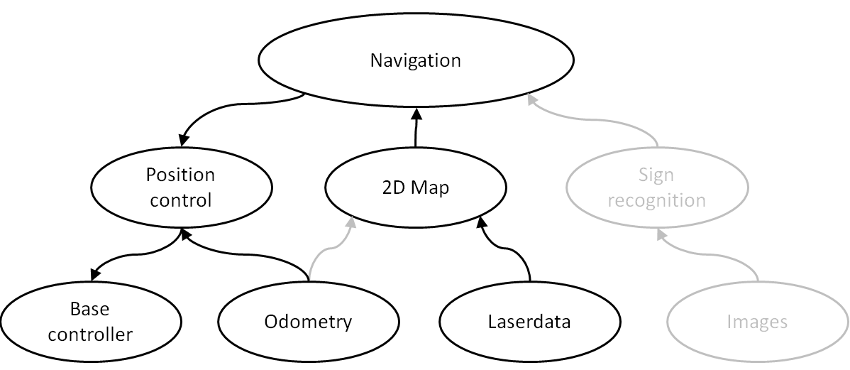
The scheme above shows the first proposal of the components of which the final program will consist. A more detailed overview will be published in the coming days or week(s). The components in grey are considered to be not very important in order to successfully complete the corridor competition. However, these components are necessary for a successful completion of the final competition.
Final structure
The final structure of the program is slightly different to the one shown above which was basically the outcome of our first brainstorm. Our current structure is shown below, where the oval shapes reperesent the node and the ones with a thick, coloured (but not blue) border are services. The navigation node actually does the navigation task and sends the velocity commands to Jazz in order to let it drive forward. Furthermore it recognizes exits and does the normal driving between two parallel walls. The node called "create dump map" constructs a map that counts the number of visits of each corridor in order to be able to perform the Tremaux's algorithm. The SLAM node is actually the gmapping node which is used to do simultaneous self-localization and mapping. Arrow detection is done by the service "Detect Arrows" and the node Hough Linedetection is used to detect walls and also an opening in a wall. Looking up the number of visits from the dumpmap is done by the service "Read dump map".
Maze solving Algorithm's
There are many ways to solve a maze. These ways of finding the exit are translated into algorithm's. An overview of these algorithm's is given here: [1].
Based on this website and on the results shown in the paper "Simulated Maze Solving Algorithms through Unknown Mazes", presented in this pdf-file: [2], we probably will tackle the problem of solving the maze by means of the so-called Tremaux's Algorithm. As a backup plan the Wall follower algorithm is chosen.
Tremaux's Algorithm
The Tremaux's Algorithm solves a maze by marking how many time a passage has been passed, when a junction is encountered that is not visited yet a random passage is chosen. If the junction is visited before the passage with the lowest counts of visits is chosen (if there are multiple options a random choice between these options is made). Exception to this is if the passage which we are arriving from is only visited once, then we will go back through the same passage, this is to avoid going around in circles.
Some pictures that clarify how the decision making is done by Tremaux's Algorithm are shown below.
 |
 |
 |
An example of why there has to be turned around at a junction at certain conditions is shown below. If at this point there is not decided to turn back, there is a change that the direction back to the beginpoint is chosen.
An example of a maze solved by the Tremaux's Algorithm is shown below, the green markers indicate a decision not made random but based on the number of visits of all the possible passages.
Wall follower algorithm
The Wall follower algorithm is a very simple algorithm to solve a maze. In the beginning a wall is chosen and this wall is followed, basicly this means start moving through a passage and if a junction is encountered alway turn right (or always turn left) if possible. Disadvantage of this algorithm is that it does not always find a solution, but the great advantage is that it is very simple to implement because it does not require a memory of which passages have been visited.
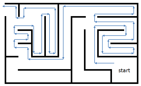
An example of a maze solved by the Wall follower algorithm is shown below.
Line Detection
To help Jazz driving straight through corridors and detecting junctions a line detection algorithm is implemented. The hough transform algorithm is the algorithm we have chosen for this, how this algorithm works and is implemented is explained here.
For every point that is detected by the laserscanner lines are drawn through that point with different angles, the distance perpendicular to the line is then measured. If for a certain angle the distances for two points are the same, these points are on the same line. This is further explained with some pictures.
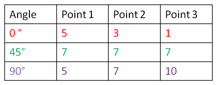
From this example can be concluded that the points or on a line with angle 45° at a distance of 7. Of course in reality more lines per point are calculated depending on the required accuracy. Also the distance does never exactly match because of measurement noise and the fact that real walls are never perfectly straight. Therefore the distance does not have to be exactly the same but has to be within a certain tolerance.
How this works for the real laserdata is explained with some pictures. First for every point the distance is plotted as a function of the angle. This angle goes from 0 degrees to 180 degrees in steps of the desired accuracy. This range can describe all possible lines like shown in the pictures below.
The implementation of this algorithm is now further explained with a captured frame of the laserdata shown below.
First all the angles and distances for each point from the laserdata are calculated, then a raster is created with all possible lines. Each element of this raster represents a line with a certain angle and a certain distance to Jazz (measured perpendicular on the line). The size of the elements of this raster depends on the tolerances for the distance and angle that have been set.
The number of points inside each element is counted. When the number of points is more than a certain threshold this is considered to be a line.
The first plot shows a graphical interpretation of all the lines that are calculated for each point. The second plot shows the raster and its elements, the points within each of these elements are counted. The elements which hold at least a certain amount of points represent a line, these are the peaks shown in the last figure.
Extraction of start and endpoints of the lines
The start and endpoints of a line are examined by appointing all the points from the laserscan to the lines the belong to. After this is done, two neighboring points are compared to see if there mutual distance is smaller than some tolerance in order to make sure that they lay on the same line section. For all the points belonging to one section, the first and last point are considered to be the start and endpoint of that particular section. The obtained information is sent to the navigation node which decides about the actions to take. The messages, defined by a new structure, that are sent by the line recognition node contain the number of lines, and for each line, the number of sections, and per section the coordinates of the begin and endpoint together with the number of points on the section.
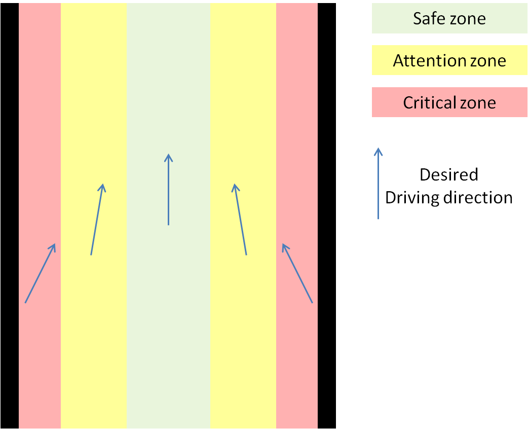
Driving through corridor
To drive safeley through a corridor without colliding into walls a corridor is virtually divided into 3 different zones.
Safe zone:
This zone is in the middle of the corridor and the desired velocity here will be at maximum allowed velocity, the desired driving direction of Jazz will be straight ahead.
Attention zone:
These zones are a bit closer to the walls, therefore the desired velocity here will be half of the maximum allowed velocity, the desired driving direction will be slightly to the middle of the corridor to get into the safe zone again.
Critical zone:
These zones are so close to the wall that there is a severe risk of colliding with the walls. The desired velocity here will be set to zero if Jazz' driving direction is still directing to the wall. If the driving direction is directing from the wall the desired velocity will be half of the maximum allowed velocity. The desired driving direction will be pretty sharp to the middle of the corridor to leave the critical zone.
The zones are illustrated in the picture below.
Junction handling
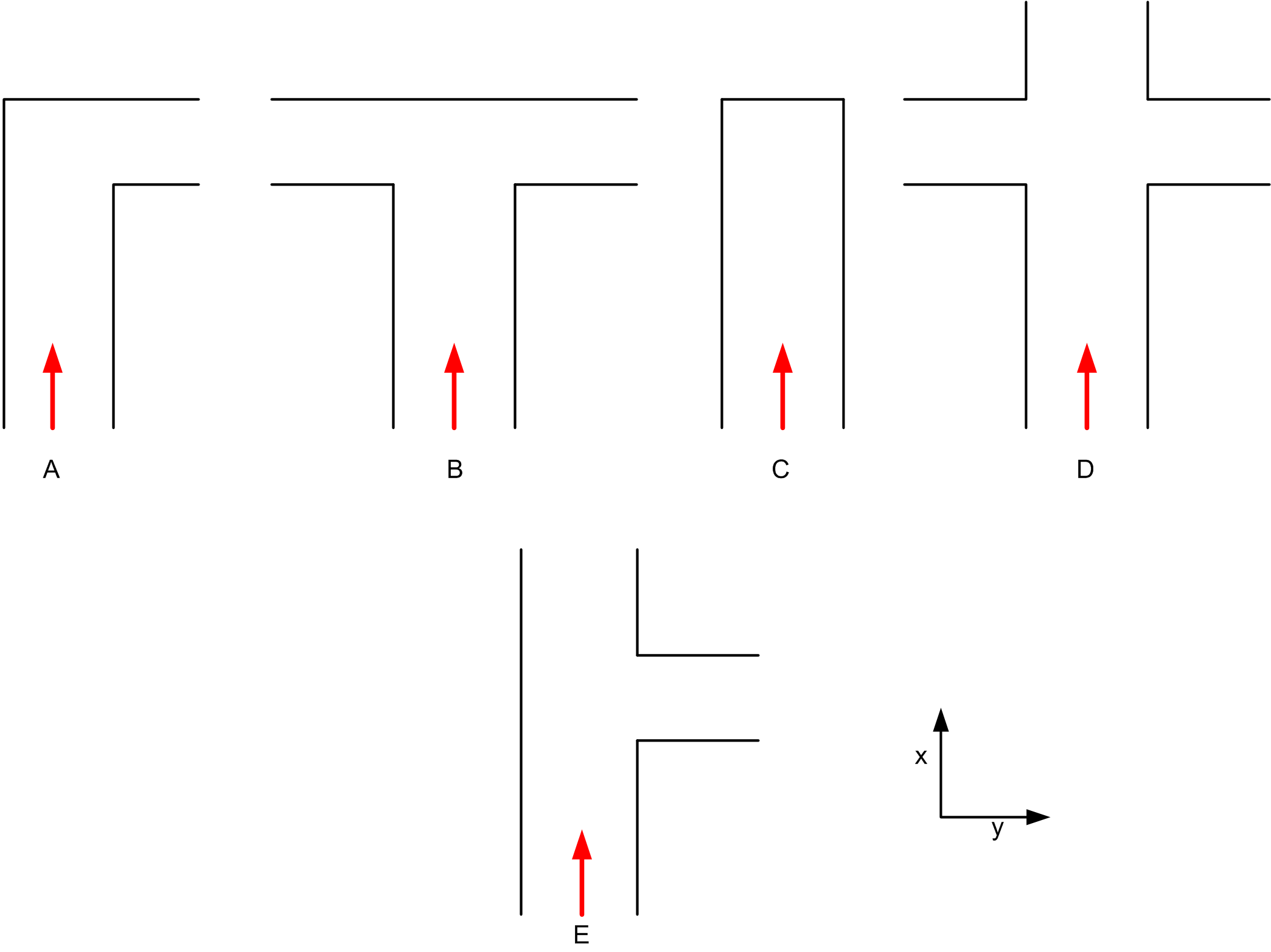
In order to succesfully navigate through the maze, an appropriate junction handler has to be designed. In our opinion, the junction handling described below will do the job: There are basically 5 types of junctions Jazz will encounter during its drive through the maze as shown in the figure below. The red arrow indicates the direction from which Jazz approaches the junction. Note that a dead end is also considered to be and handeled is if it is a junction.
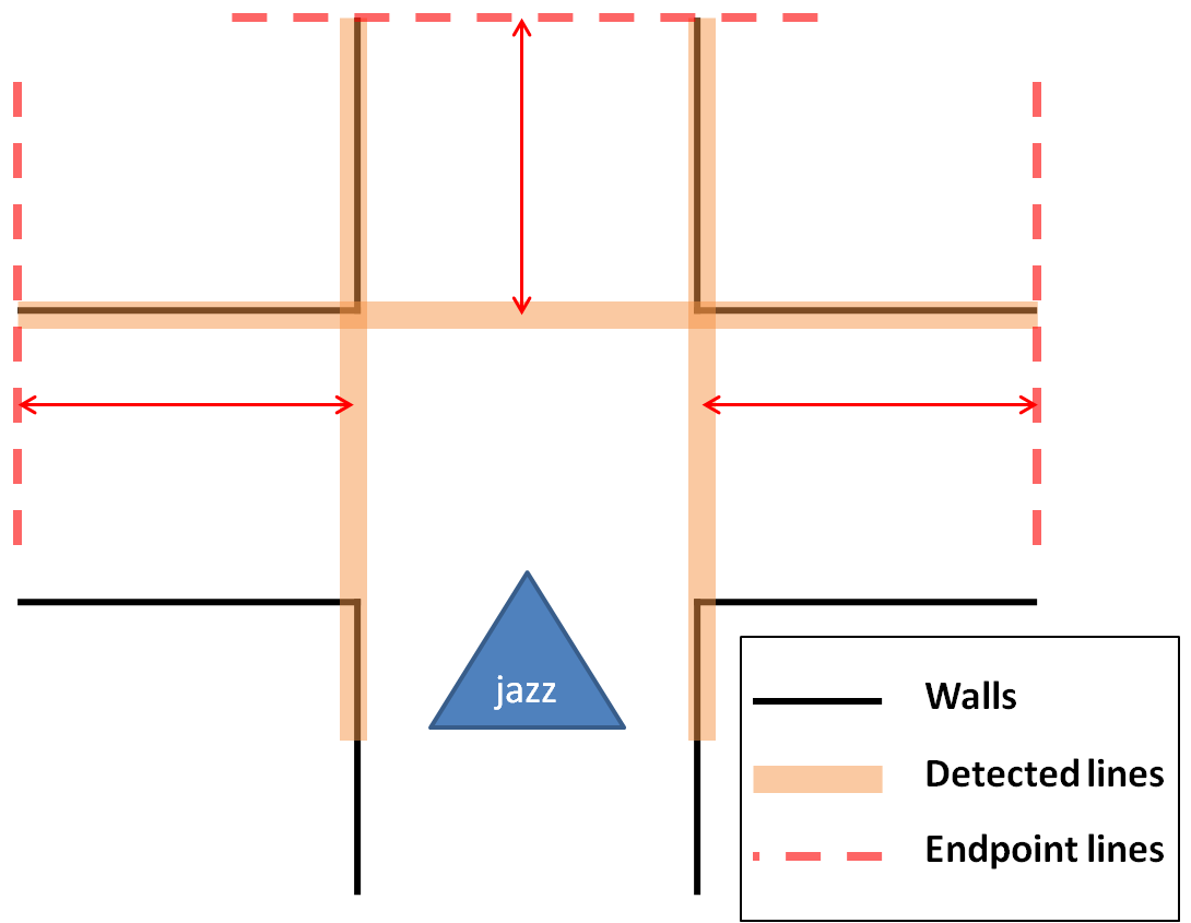
The recognition of the different situations is planned to do in the following manner:
- A junction is detected when a line at an angle of approximately 90 degrees is found, this line is referred to as an 'exitline'.
- A line parallel to the side walls is drawn at the right end of this exitline, then the distance between this line (red dashed line in the image below) and the right wall is calculated. If this distance is larger than a certain tresshold, a right exit exists.
- This is also done on the left side.
- To check for front exits a line is drawn parallel to the exitline at the end of the lines at the side walls. The distance between this line and the exitline is calculated and if this distance is larger than a certain tresshold, a front exit exists.
- Based on which exits are found the situation is determined.
Based on the junction type detected, the appropriate action should be taken, such as drive forward, turn left/right, check for an arrow and check each passage for the number of visits.
Robustness Measures
In order to make the junction recognition robust and also working in case of minor deviations from the ideal situation we have taken some measures. The most important measures are explained below. Note that these are additions to the original proposed method, as this method worked fine in ideal cases but not for a whole maze with a seris of junctions connected to each other.
- Paralell lines which are used by Jazz to recognize the walls between which it drives are limited to a distance of 1 meter, in order to make the right distinction between for example a corner and a dead end in case of coupled junctions.
- If only one side wall is detected, the previously measured hallwidth is used to approximate the position of the other side wall.
- Decisions are made only after one type of exit is recognized 2 times, to prevent Jazz from taking a wrong decision if a line is once not recognized properly.
- Finally, the line at an angle of 90 degrees is always the nearest line at 90 degrees, which may otherwise also cause trouble in case of connected junctions.
Implementation of Tremaux's Algorithm
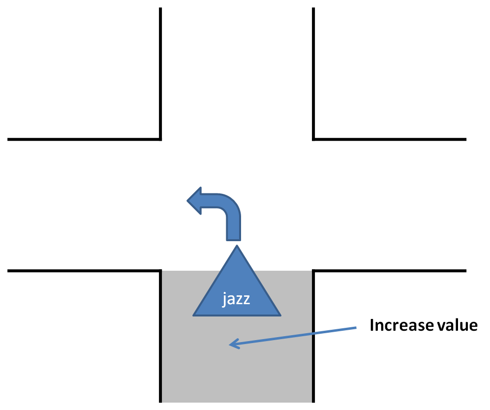
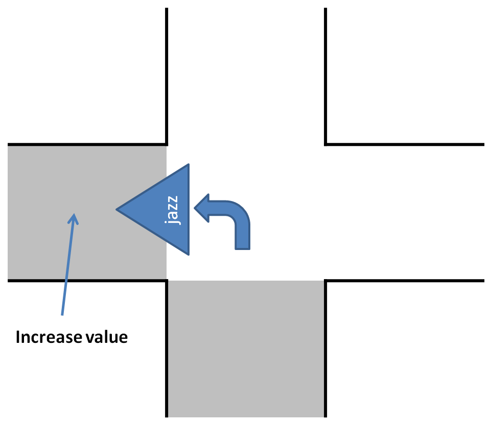
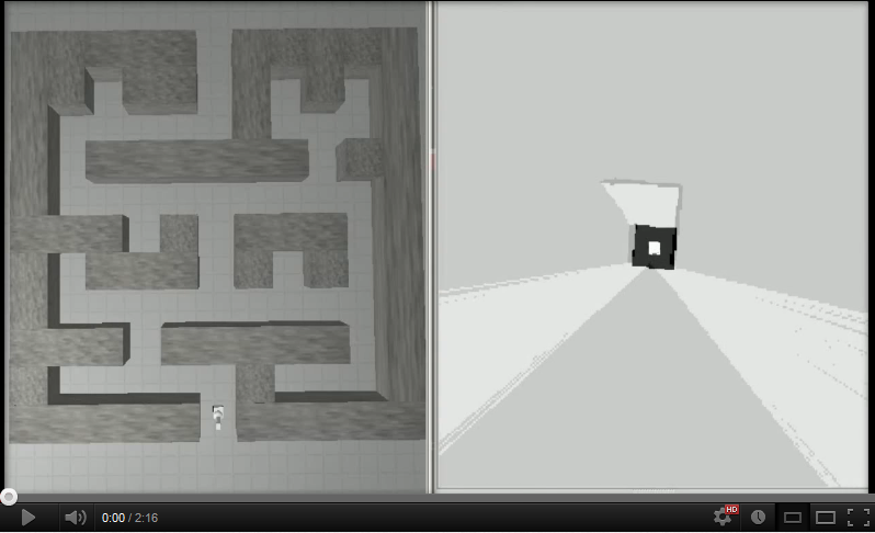
In order to use Tremaux's Algorithm to solve the maze a map is made to remember the number of visits per corridor. The SLAM algorithm from gmapping is used to determine the position of Jazz, because the odometry is not reliable. The navigation node gives order to the 'create dump map' node whenever it leaves or enters a corridor to increase the value that indicates the number of visits. The 'create dump map' node then checks the current value and increases that value. The 'read dump map' service is called by the navigation node whenever a junction is encountered, this service then returns the number of visits of all corridors at the encountered junction. Pictures and a video are shown below to illustrate how this is implemented.
 |
 |
Arrow recognition
The detection of the arrows will be done by detecting the corners of the arrow. First, we did a simple test in Matlab with a photo of an arrow, using the Image Processing toolbox of Matlab. And now we are trying to write a corner detection algorithm for ROS. Probably using the "cornerSubpix"[3] function of the OpenCV library. We will use a simple webcam to test our algorithm. To be able to use a webcam in ROS the following tutorial is followed: [4].
Update* We will only check for arrows in the neighborhood of a junction, to avoid unnecessary image processing. Only a the time that a t-junction is detected by Jazz the Arrow algorithm will be called. Then the Arrow algorithm should detect the possible arrow between 1.2m (when the T-junction is detected) and 0.5m (when Jazz is commanded to take a turn) before the wall. How the arrow will be detected is described below, in this section a brief summary of the Arrow algorithm is given.
Arrow algorithm
Step 1.) Compensate for distortion fish-eye lens
 |
 |
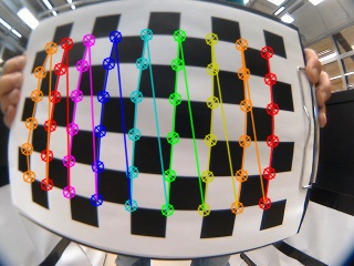
The provided images taken with the camera of Jazz have not a really high quality partially due to the so-called fish-eye effect which causes a distortion. Distorted arrows may be hard to recognize and as the camera properties will most likely not change, we have used to solve this issue by correcting the distortion by a calibration as is described on this webpage: Camera Calibration example a other webpage is Information on distortion Correction. The calibration with the images below is not perfect, because of there were no image captured on the side of the camera.
Step 2.) Resize image 2x bigger
After lots of testing with our arrow detection algorithm we were still not satisfied with the result. Not because our arrow detection did not work, but because our detection was limited to a small range. Only in less then 1 meter from the arrow we were able to detect the direction of the arrow. The main reason for this is that the resolution of the camera is not so high. Therefore we decided to use linear interpolation to increase the resolution of our input image. We used the function Resize[5] to increase the resolution in both directions with a factor 2.
We do not get more information with this function, but with a higher resolution we were able to detect more corners. And therefore we got a better determination of the direction of the arrow.
 |
 |
Step 3.) Convert image to HSV image
 |
 |
HSV varies the hue component of the hue-saturation-value color model. The colors begin with red, pass through yellow, green, cyan, blue, magenta, and return to red. The advance of using HSV is that you can use a color for different illuminations by using a hue and saturation value. We used is so we are sure that we are looking for a red object. With the saturation and value it is possible to be less sensitive to light.
|
|
|||||||||||||||||||||||||||||||||||||||||||||||||||||||||||||||||||||||||||||||||||||||||||||||||||||||||||||||||||||||||||||||||||||||||||||||||||||||||||||||||||||||||||||||||||||||||||||||||||||||||||||||||||||||||||||
|
|
||||||||||||||||||||||||||||||||||||||||||||||||||||||||||||||||||||||||||||||||||||||||||||||||||||||||||||||||||||||||||||||||||||||||||||||||||||||||||||||||||||||||||||||||||||||||||||||||||||||||||||||||||||||||||||
|
|
||||||||||||||||||||||||||||||||||||||||||||||||||||||||||||||||||||||||||||||||||||||||||||||||||||||||||||||||||||||||||||||||||||||||||||||||||||||||||||||||||||||||||||||||||||||||||||||||||||||||||||||||||||||||||||
|
|
||||||||||||||||||||||||||||||||||||||||||||||||||||||||||||||||||||||||||||||||||||||||||||||||||||||||||||||||||||||||||||||||||||||||||||||||||||||||||||||||||||||||||||||||||||||||||||||||||||||||||||||||||||||||||||
Step 4.) Convert red pixels to black and white image
 |
 |
From the HSV image we create a black and white image (binary image). In the tables above you can see which values to use if you only want to find red arrows. We implemented a track-bar for each parameter to find easily the ideal parameters settings for a variety of conditions. This resulted in the following boundaries for each parameter:
[math]\displaystyle{
(H \leq 16 \vee H \geq 343) \land S \geq 0.50 \land V \geq 0.50
}[/math]
Step 5.) Find biggest contour
Afther the conversion of the HSV image to a binary image there was still some noise in our image. Probably as a result of reflection of the light and the presence of other red objects near the red arrow. Therefore we search in the binary image for closed contours, i.e. for object pixels that are connected with each other, using the FindContours[6] function of OpenCV. For each contours we calculate the area and store the biggest contour. We use a threshold value (a minimum area) the biggest object must have to proceed with the algorithm. Since from a far distance the shape of an arrow is not clearly visible. This is also prevented by only calling the Arrow algorithm at a short distance from a t-junction. Since only the biggest contour remains the residual noise is filtered out and only a possible arrow is left.
 |
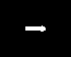 |
Step 6.) Region of interest
 |
 |
Region of Interest is a rectangular area in an image, to segment object for further processing. The ilustration is shown in Figure 1 below. For speeding up the algorithm we take 50 pixel up, down, left and right bigger as the boundaries of the contour. So that the watershed segmentation cannot segment something what is not red or not interested in.
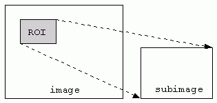
Step 7.) Watershed segmentation
 |
 |
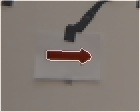 |
We have used the watershed segmentation so we get a all the information of the arrow possible out of the image at a bigger distance.
The are different approaches may be employed to use the watershed principle for image segmentation.
- Local minima of the gradient of the image may be chosen as markers, in this case an over-segmentation is produced and a second step involves region merging.
- Marker based watershed transformation make use of specific marker positions which have been either explicitly defined by the user or determined automatically with morphological operators or other ways.
We have used the Marker based watershed transformation.
Step 8.) Match the shape of the contour with a template arrow
If a contour is found does this not directly mean that it is also a arrow. Therefore the function MatchShapes[7] is used to compare the shape of the contour with a predefined template arrow. This function calculates the rotation invariant moments[8] (Hu moments) of each possible arrow that we get. Then the function compares the Hu moments with the Hu moments of a template arrow which we recorded earlier. And compares these two sets of Hu moments and gives a result in the form of a certain value. The lower the value (ideally is 0) the more similarities between the two Hu moments and thus the more simularities between the two shapes. A lot of testing is done to find an reliable maximum value.
The advantage of the Hu moments is that they are invariant under translation, changes in scale, and also rotation. So this MatchShapes function will also work properly with slightly rotated arrows or when the detected arrow is of a different size than the template arrow. Or even when the arrow points to the other direction then our template arrow.
Step 9.) Corner detection
To detect the direction of the arrow we use the function Cornersubpix[9] to calculate the corners of the arrow. Based on this corners we determine the direction of the arrow, by looking at which side the most corners are found. Because the resolution of the arrow is still not perfect, the function Cornersubpix sometimes detects corners along the edge in the middle of the arrow. Which also can be seen in the picture below. Therefore we implemented a filter which filters out the corners which are detected within a certain area around the centre point of the arrow. With the result that only the actual corners of the arrow are left, resulting in a correct detection of the direction of the arrow.
 |
 |
Overview process
 |
 |
 |
 |
 |
 |
 |
 |
Video of testing arrow algorithm
We have recorded two video's while running the arrow detection algorithm. The first one was the first test with a bag file. Not al the functions we discussed above were implemented yet during this test. The second one is our final test. With a driving Jazz robot controlled by the remote control.
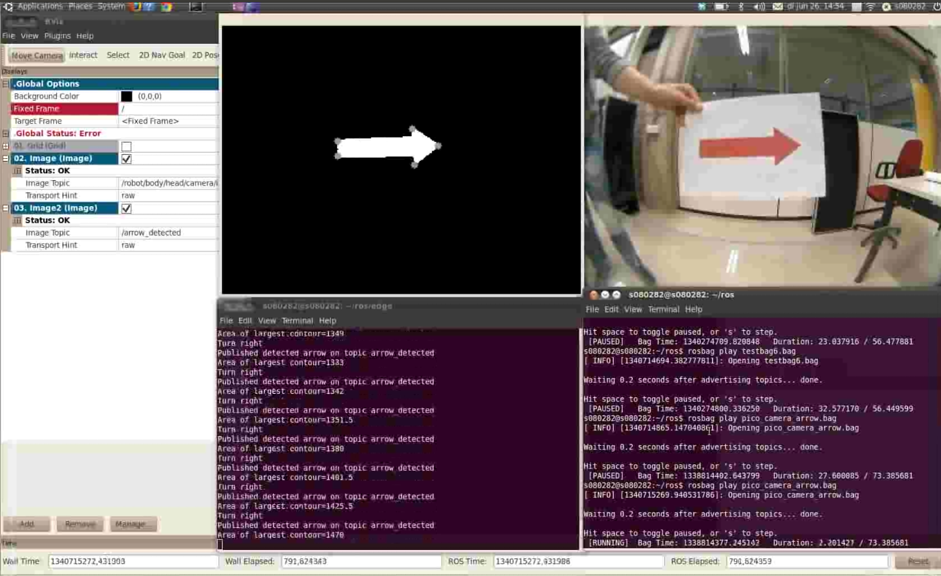
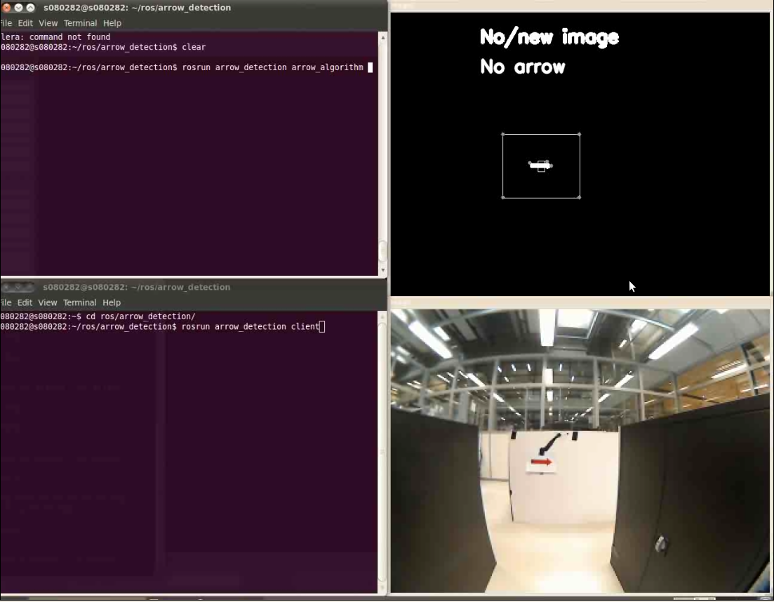
Overall algorithm
Driving fases
Initialisation fase
This fase only runs in the beginning and in some failsafe cases (see below). During this fase Jazz finds the line that is closest and turns untill its heading direction is parallel to this line. The initialisation fase then ends and the parallel driving fase starts.
Parallel driving fase
In this fase Jazz tries to move parallel to the closest parallel line. This is achieved by controlling the radspeed dependent of the difference in angle between the driving direction and the parallel line (shown below). If Jazz is not in the safe zone an offset is given to this angle to move towards the safe zone. The forward velocity is also dependent of the zone where Jazz is in.
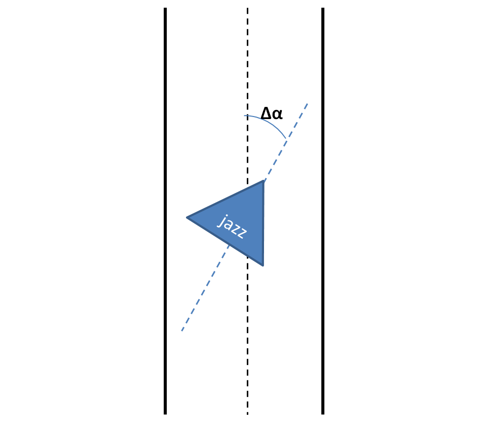
Turning fase
In this fase Jazz turns left or right. The turning fase has two subfases, in the first fase Jazz does not start turning yet but moves towards the exitline (shown in the picture below) untill the distance to this exitline is half the hallwidth. Then the forward velocity is set to zero and Jazz begins turning, this is done by controlling the radspeed bependent of the difference in angle between the driving direction and the exitline. The angle with this exitline is monitored and if it is close to parallel the turning fase ends and the parallel driving fase starts.
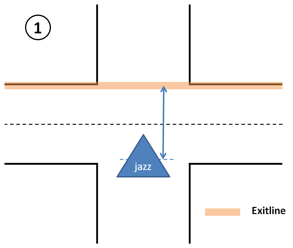 |
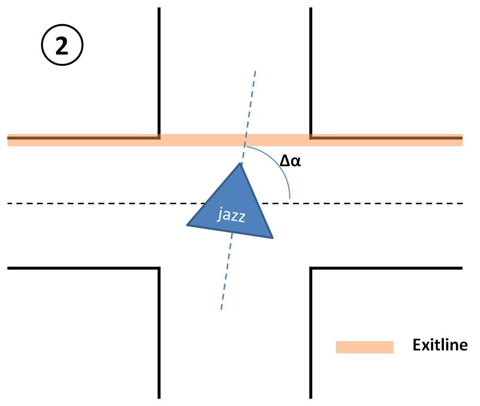 |
Dead end fase
In this fase Jazz turns 180 degrees drives back into the corridor where it came from. The forward velocity is set to zero and Jazz starts turning untill it is parallel in the corridor again. How this works is shown in the picture below.
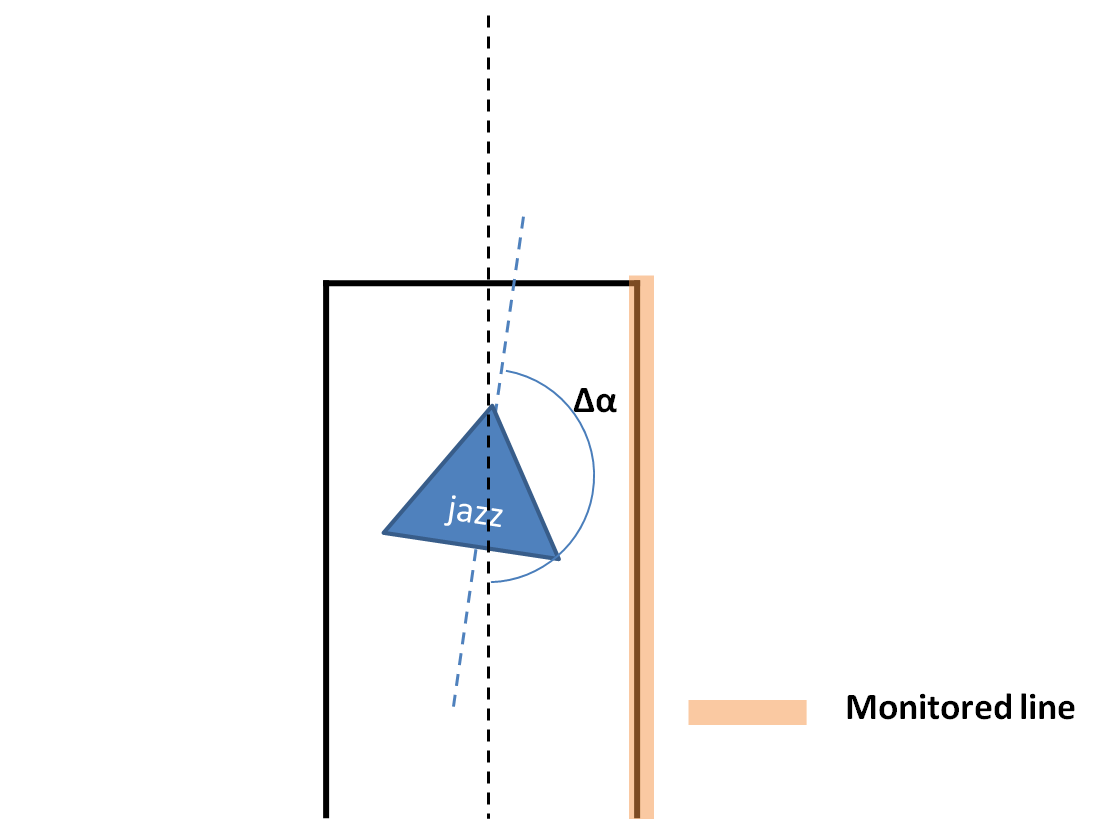
Exit detection
The exit detection searches for lines that are at an angle of approximately 90 degrees. If a line like this is found the type of junction is determined and if this is done the exit handling starts. The exit detection is then suspended untill Jazz has moved out of the current junction. This is done by monitoring a line that cannot be detected anymore when Jazz has moved out of the junction, so when this line cannot be monitored any more the exit detection is not suspended anymore. Which line this is is shown in the picture below.
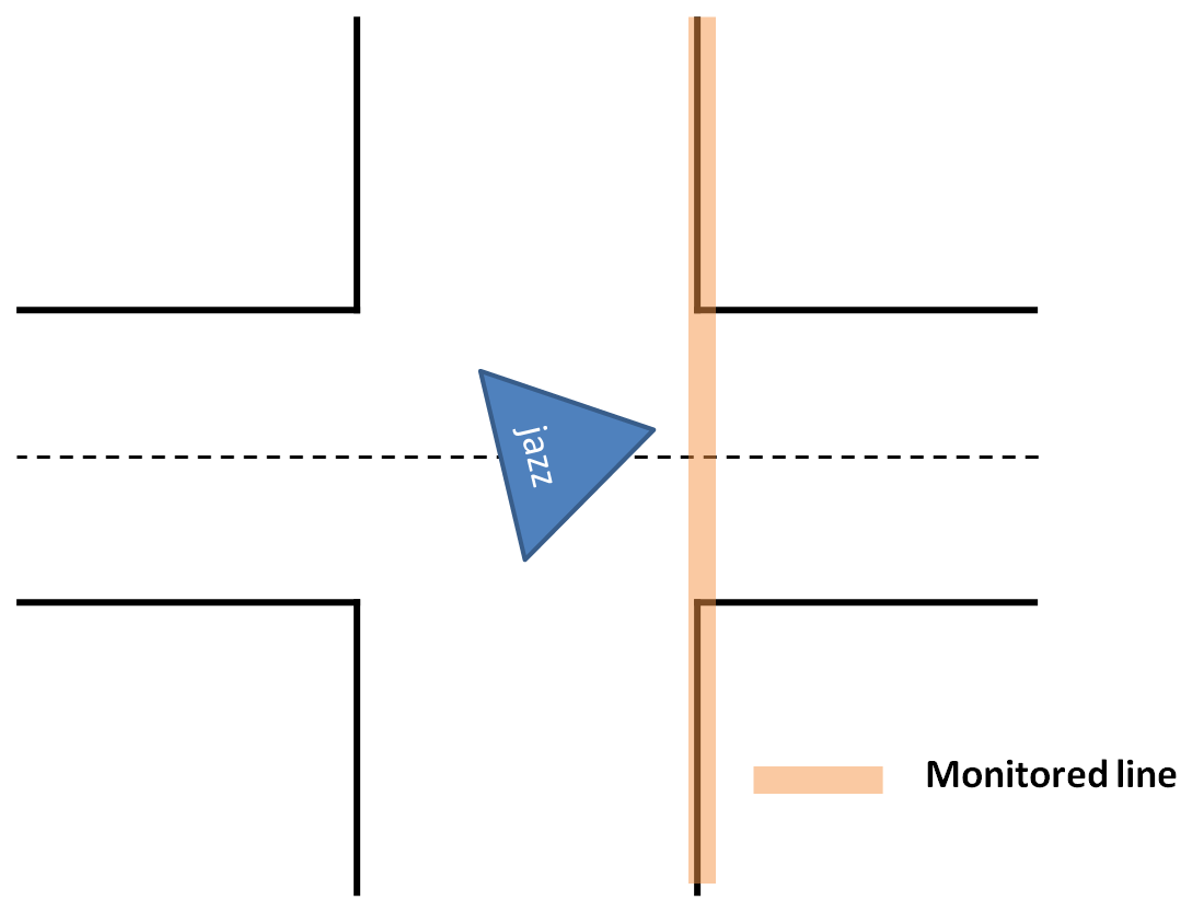
Arrow detection
The arrow detection is only called when a T-junction is detected, because this is the only place where the arrows could be placed. The arrow detection service then returns a value 0, 1 or 2. 0 means there is no arrow detected, 1 is for a left arrow, 2 for a right arrow. How this arrow is used is explained in the exit handling below.
Exit handling
The exit handling is executed when an exit is detected. It receives data that contains information about where the exits are and how many times they have been visited before and the arrow direction. The exit handling decides which exit to take by using Tremaux's algorithm, so it picks the exit with the least amounts of visits. When the exits have the same amount of visits the exit normally should be picked randomly according to Tremaux's algorithm. However we have chosen that if there is a front exit, this exit should be preferred because turning takes more time. If there is no front exit or this exit has more visits, left and right are picked randomly. An exception is made for when an arrow is detected, the direction of the arrow is then preferred. When the direction of the arrow has more visits than one of the other exits, the arrow is ignored. This is to ensure that the maze will be solved, even when an arrow is detected wrong.
Fail-safes
To prevent deadlocks or collisions some fail-safes are introduced.
- Laserdata age: If the received laserdata is older then 500ms Jazz stops moving and waits for new laserdata.
- Monitored lines are not found: If lines that are monitored and disappear when they are not expected to (this is during the turning or dead end fase), Jazz stops moving for 1 second. If the line is not found within this second Jazz goes back to the parallel driving fase.
- No parallel lines are found: If during the parallel driving fase no parallel lines are found, Jazz stops moving. If there are no parallel lines found within a second Jazz goes back to the initialisation fase.
- No lines detected: If there are no lines detected at all, Jazz stops moving. If no lines are detected within 5 seconds Jazz slowly starts rotating untill one or more lines are detected.
- Arrow detection service fails: If the arrow detection service fails or is not running Jazz can still function by using only Tremaux's algorithm.
- Dump Map service fails: If the map service fails or is not running Jazz can still function by switching to the wallfollower algorithm.
Simulation versus real world
Temporarily solution for the laserdata points
Because we encountered some unexpected problems during the first test on the real robot we have made some modification to the simulator so it becomes a better representation of the real world. Our line detection uses the laserdata as an input and was optimized for the laserscanner of the simulator which returned 180 points. The real laserscanner returns 1080 points, which our program could not handle. To prevent this problem in the future an extra program is written that takes in the 180 points laserdata from the simulator and transforms this to 1080 points laserdata. This is done by lineair interpolation between the points of the simulated laserdata.
The visualisation of the new laserdata is shown in de picture below, the red dots represent the points from the new simulated laserdata, the white dots are those from the old simulated laserdata.
Walls
We also made a corridor in the simulator that does not have perfectly straight walls, because in reality this is also not the case. For testing the robustness of our line detection algorithm this is very useful. The difference between the old and new corridor world is shown below.

Modified corridor world with walls that are not perfectly straight.
Synchronisation issues
To make sure our algorithm worked properly some messages had to be synchronized, this all went well in the simulator. In the real world test the messages would not synchronize in some cases, this was caused by the fact that the program ran on an external workstation. Both the workstation and Jazz have their own system time and some messages received their time stamp from Jazz' system time and others from the workstation's system time. These messages can not by synchronized properly. We decided to take out the synchronization and during the tests this went well, but this is no guarantee that it will never cause problems.
Communication delays
Because the control of Jazz is executed on an external workstation Jazz suffered from communication delay. Because of this delay we decided to increase the critical zone of the corridor and tune down some parameters which resulted in a slower moving Jazz. This was the only way to make Jazz stable. In the final competition our Jazz moved very slowly but also was the only one which made it through the maze. With some more test time we would be able to make it a bit faster, but the delays in communication were the most limiting factor.
Presentation Final competition June 29th 2012
Jazz's Blog
In this section I will publish all kinds of information on the things I am currently learning, I have learned so far and my further ambitions.
29th of June 2012 – I won the final contest!
It was an awesome day today. I was able to complete the final contest within the fastest time. Not everything went perfect because some parameters of my program were not optimized due to limited test time, nevertheless I have made me and my bosses very proud. Look at the video below to see me driving through the maze.
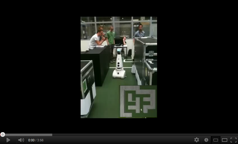
27th of June 2012 – Final tests
Today, I had my last oppertunity to test in a real maze, and as last Thursday my communication suffered again from delays up to a 4 seconds, even by calling just "pico ping". But after reporting this situation someone passed by who fixed this issue of netwrok overload, and afterwards, my tests went pretty well as I can drive through the maze completely autonomously while making a map and looking up how many times an exit is visited at a junction. The arrow recognition is not robust enough yet, but I have some ideas on how to improve robustness for the final competition! Will be continued...
26th of June 2012 – Achieved one of my ultimate goals!
It was a great day today, as I succeeded to solve several maze's in simulation using Tremaux's algorithm, with different types of junction handling in case of an equal number of visits of several directions at a junction. A video is shown below and I hope to achieve this also in the experiments. So, hope to have more good news later...

21th of June 2012 – Real world test 3
Today, I had my third test event, but that was not a big succes. The communication between me and the computer suffered from HUGE delays up to 10 seconds and more. Sometimes the communcation broke down completely. However, once the communcation was up and running properly the test were a succes, except for a missing transform needed to test the mapping algorithm implemented to perform the Tremaux's Algorithm. This issue is solved yet so I hope to show you some evidence in the coming few hours or days.
18th of June 2012 – First step towards Tremaux's Algorithm
In order to use Tremaux's Algorithm, I successfully can draw points on a map at the position I currently visit and store it in my memory. I will extend this tomorrow to coloring the full corridor and finally detecting the number of visits.
14th of June 2012 – Real world test 2
Today I had my second day of real life testing and I recognized all types of junction separately. However, some connected junctions gave some trouble but in the meanwhile I have figured out some measures to overcome the problem. There is also quite some progress made in the arrow recognition, as I can detect the arrows on almost all of the provided pictures, including their direction. I am still studying to improve the robustness and to see how I can make a map in my memory in order to apply Tremaux's algorithm. Will be continued...
12th of June 2012 – Travelled through the maze
autonomously
Finally, I have learned how to drive through the maze without any intervention from outside. I travelled through the maze by means of the wall follower algorithm, following the right wall. This strategy is also known as the right-hand-rule. I will post a video soon to give you some evidence...
Here my evidence is:
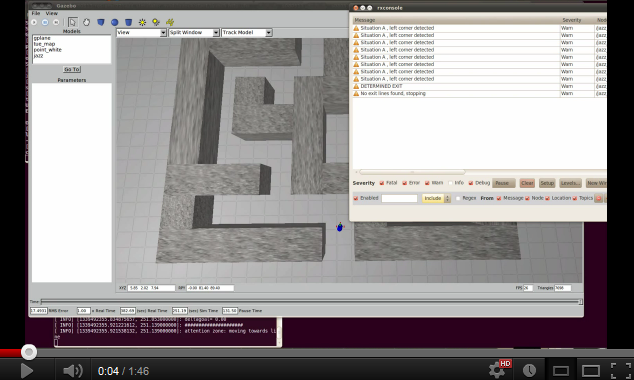
As in all cases, I can improve myself and I definetely will do during the coming days. Moreover I have planned to see if I also can learn how to apply to Tremaux algorithm to prevent endless searching in bigger mazes with more junctions and exits.
5th of June 2012 – Recognition of the junction types
Today, I have learned to recognize the different types of junctions described in the section junction handling. I have only to pay some more attention to see at which side the corner (junction type A) is directed and at which side the exit is in case of junction type E. Will be continued soon...
In the meanwhile, I have also overcome the challenge of detecting the side of the exit for junction type A and E. Now, I only have to recognize arrows and look at the map to take appropriate actions according to Tremaux's Algorithm. See the video below of how I am detecting the junction types.
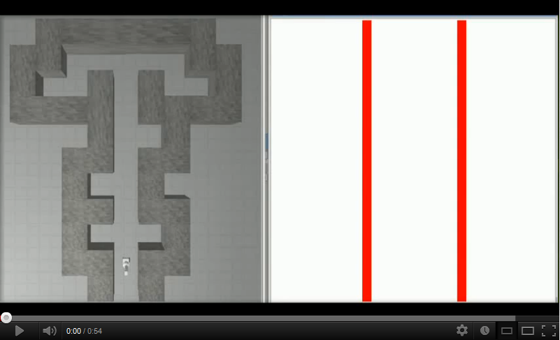
4th of June 2012 – I passed the corridor challenge!!
A small step for men, a huge step for me: Today I passed the corridor competition in 1 minute and 40 seconds. This was not the fastest time, but that was due to the fact that I had no time to practice due to an error. See the video below of me going through the corridor.
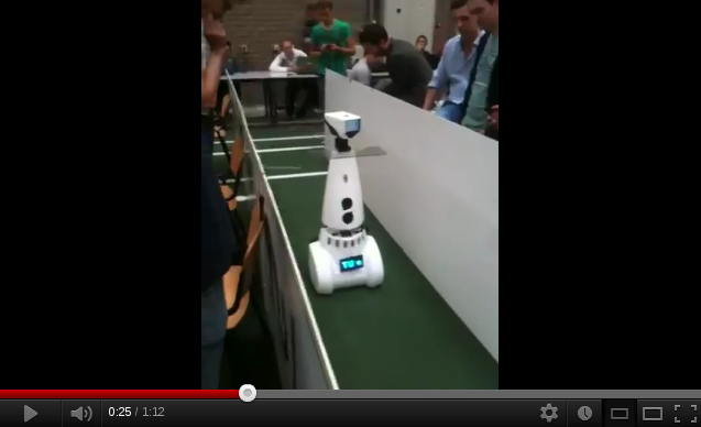
1st of June 2012 – Drove autonomously through the corridor and exit
I drove autonomously through the corridor and turned towards the exit. I also kept aligning myself during my drive in the corridor, such that I drove at the center of the corridor. See this video for a prove:
During the real world tests, I had a memory problem so this test failed for me but I have solved this yet. So hope for better luck on Monday. To be continued...
31th of May 2012 – Driving centered through a corridor
I made again a leap forward in solving the maze problem. I succeeded in driving at the center of the corridor and staying at the center while driving on. Hope to learn also to make a turn at a junction later today...
30th of May 2012 – Wall detection 4
Yesterday, I finally managed to find the begin and endpoints of the walls in a proper way. To see how I can detect lines now watch the video below:
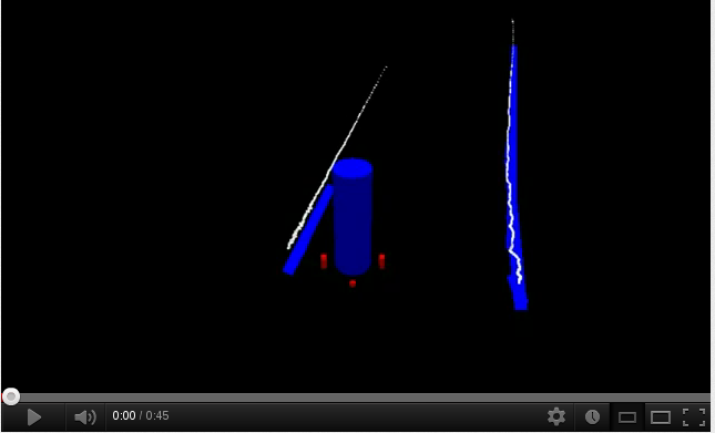
Currently I am trying to figure out how I can ride through the maze without bumping into the walls while making nice corners at a junction. In the meanwhile I am also still studying how to process my camera images to detect the pointing direction of the arrows. To be continued soon...
24th of May 2012 – Wall detection 3
Today, I have detected the direction of and distance to walls, seen from processing the laser scan data. I now only have to figure out where the walls end in order to recognize an exit and pass the corridor compition succesfully!! Recognition of the end of a wall I will do by selecting the laser data points which belong to a certain line and looking at the first and last point of the selection. Therefore I also have to check whether a line is splitted in to more sections, or wheter it is just one solid line. Hope to get this done by the weekend!!
22th of May 2012 – Wall detection 2
I am still struggling with detecting all the walls from the laser scan data. I changed my plan and I will probably use a homemade piece of code to detect the lines, based on the socalled Houghtransform. I prefer this method above the ransac method, as I mentioned last week, since it is capable of detecting more lines at one evaluation. Besides, I am still trying to make the arrow recognition more robust. However, I can recognize an arrow with some images stored last week, but it does not work with all new images.
I hope to have some progress in the coming days, as the corridor competition comes closer and closer! To be continued...
18th of May 2012 – Detecting the walls
Today I managed to find the position of the walls of the corridor while I was walking through. Even without hitting the walls, which is of course a big leap forward on the way to my ultimate goal: escaping from the maze. I employed the point cloud library of ROS and especially the RANSAC method in order to detect the position of the walls.
16th of May 2012 – Thoughts about maze solving algorithms
Yesterday I watched the fairy tale ‘Hans and Gretel’ and I was intrigued by their idea to mark the path they had walked to find their way back. However they were not solving a maze, I can use this path marking to help me solve the maze. Of course, because I am a robot without arms I cannot drop pebbles like Hans did, but because I already learned how to create and remember a map, I can use this map to mark the passages I have already visited.
Because I also have to recognize walls and junction to solve the maze I am now trying to recognize lines in the laserdata which I receive from my sensors. Once I have learned all this I can use the Tremaux’s Algorithm to solve the maze. If I am not able to learn all these things in time I can use the Wall follower algorithm as a backup plan. These algorithms are further explained in the ‘Maze solving Algorithm's’ section.
11th of May 2012 - Created my first map
Today, I created my first map while being controlled by some keyboard inputs to steer forward, left and right. Here is a movie of this mapping process:
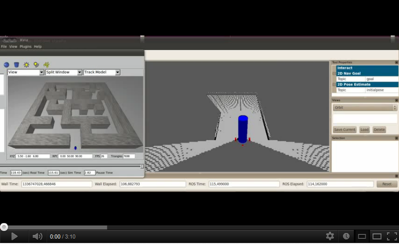
Currently, I am busy with learning how to process the map to enable navigating trough the maze. Moreover I am learning how to process images captured by my camera, such that I can recognize arrows and their pointing direction.
Next week, I'll update you about my progress...
8th of May 2012 - Learning how to make a map
Today, I have been busy with learning how I can produce a 2D map of the data I receive from all my sensors. I hope to succeed in making a map before the end of this week. Besides, I will try to succeed in driving a predefined distance or angle. This should eventually help me following the instructions of my navigation program.
I hope to have more exciting news soon...
