Embedded Motion Control 2012 Group 1: Difference between revisions
No edit summary |
|||
| (26 intermediate revisions by 3 users not shown) | |||
| Line 57: | Line 57: | ||
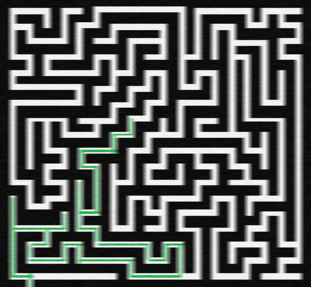
* Started with map-processing to build up a tree of the maze which can be used by the decision algorithm. | * Started with map-processing to build up a tree of the maze which can be used by the decision algorithm. | ||
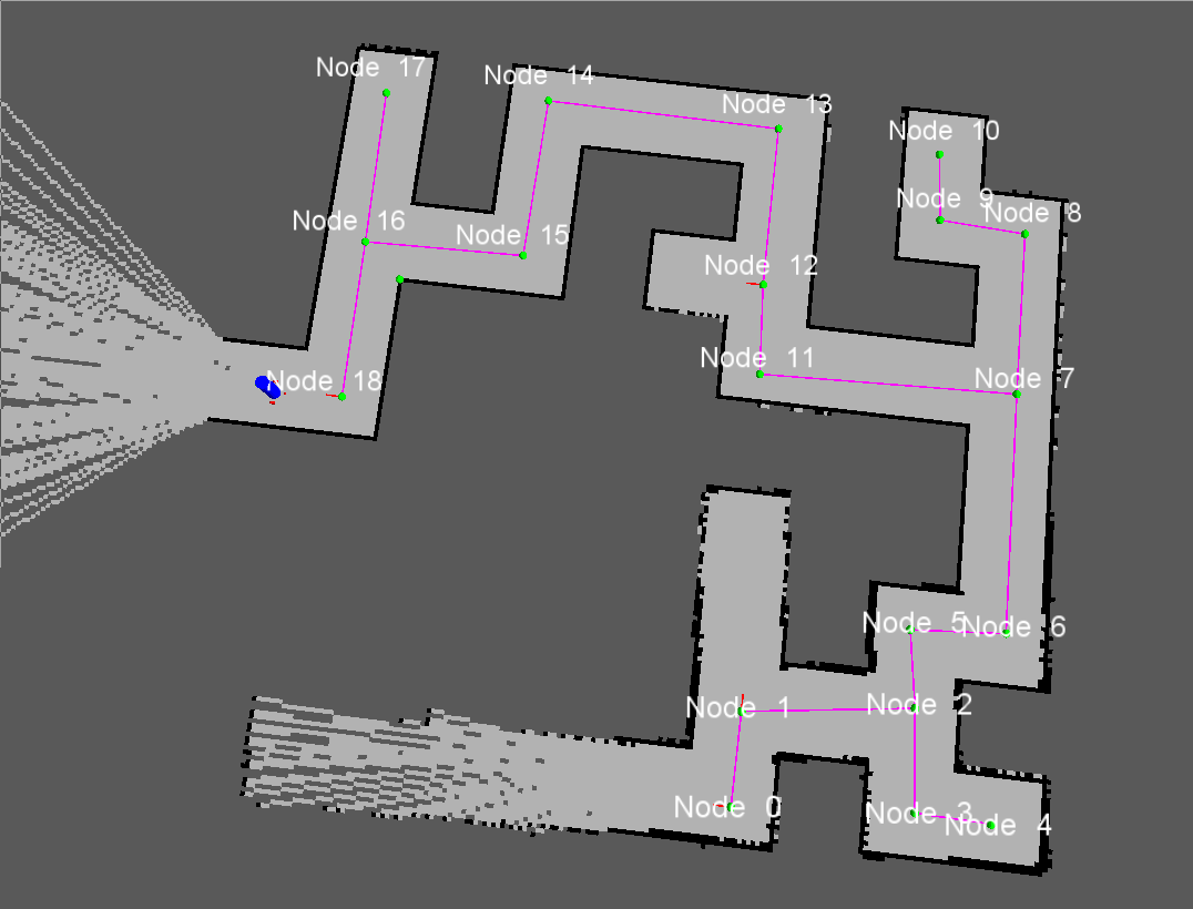
* Optimized mapping algorithm and did some processing on the map. See Figure "Optimized map" | * Optimized mapping algorithm and did some processing on the map. See Figure "Optimized map" | ||
* | * Started with navigation node for autonomous navigation of the jazz | ||
Tasks for Week 4: | Tasks for Week 4: | ||
* Process map | * Process map | ||
| Line 68: | Line 68: | ||
{| style="color: black; width="100%" class="wikitable" | {| style="color: black; width="100%" class="wikitable" | ||
| colspan="2" | | | colspan="2" | | ||
====Week 4==== | ====Week 4==== | ||
* Arrows can be detected by camera with use of the OpenCV package. | * Arrows can be detected by camera with use of the OpenCV package. | ||
| Line 116: | Line 117: | ||
* First test on Jazz robot, see right movie | * First test on Jazz robot, see right movie | ||
|[[File:Movie4_emc01.png|200px|thumb|http://www.youtube.com/watch?v=tgHOjsxDUjk&feature=plcp]] | |[[File:Movie4_emc01.png|200px|thumb|http://www.youtube.com/watch?v=tgHOjsxDUjk&feature=plcp]] | ||
| | |[[File:F3.PNG|200px|thumb|https://www.youtube.com/watch?v=HjW0VavlWrg&feature=plcp]] | ||
|} | |} | ||
{| style="color: black; width="100%" class="wikitable" | {| style="color: black; width="100%" class="wikitable" | ||
| colspan="2" | | | colspan="2" | | ||
====Week 9==== | ====Week 9==== | ||
* Simulated all possible maze cases, see | * Simulated all possible maze cases, see movies | ||
** Loop | ** Loop | ||
** Double loop | ** Double loop | ||
| Line 129: | Line 131: | ||
* Update on wiki | * Update on wiki | ||
* Could not do any testing, because set up was not working | * Could not do any testing, because set up was not working | ||
| | |[[File:F1.PNG|200px|thumb|https://www.youtube.com/watch?v=e1CASyzed3E&feature=plcp]] | ||
|[[File:F2.PNG|200px|thumb|https://www.youtube.com/watch?v=qrbDDAJchS8&feature=plcp]] | |||
|[[File:F4.PNG|200px|thumb|https://www.youtube.com/watch?v=XwLcYULewZ8&feature=plcp]] | |||
|} | |} | ||
{| style="color: black; width="100%" class="wikitable" | |||
| colspan="2" | | |||
==Navigation== | ==Navigation== | ||
| Line 159: | Line 166: | ||
====Detection corners==== | ====Detection corners==== | ||
[[File:CheckCorners.png|thumb|500px|''Corner detection'']] | |||
=====Determine CornerType===== | |||
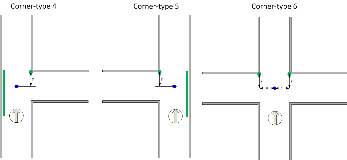
If the robot arrives at a crossing, a specific algorithm is triggered to determine the type of the crossing. The algorithm determines the cornerType which use of three variables (as can also be seen in the left figure): | |||
<ol> | |||
<li><b>frontCheck:</b> This variable denotes if the laser bundel on the north side of the robot detects any close objects. This boolean is determined with use of an average distance and a specific treshold.</li> | |||
<li><b>leftCheck:</b> This variable denotes if the checkSideCorner() algorithm finds an opening on the left side.</li> | |||
<li><b>rightCheck:</b> This variable denotes if the checkSideCorner() algorithm finds an opening on the right side.</li> | |||
</ol> | |||
Based on these three booleans, the cornerType can be determined using some logical operators. | |||
The pseudo code algorithm to detect the sideCorners is given below: | |||
'''loop''' over specific range of laser data points: | |||
'''if''' we look at the left side: | |||
'''if''' distance[i] > distance[i+1] AND distance[i]/distance[i+1] > ratioTreshold: | |||
Do some extra checks | |||
'''if''' extraChecks succeed '''then''' return true '''end''' | |||
'''end''' | |||
'''end''' | |||
'''if''' we look at the right side: | |||
'''if''' distance[i] < distance[i+1] AND distance[i]/distance[i+1] > ratioTreshold: | |||
Do some extra checks | |||
'''if''' extraChecks succeed '''then''' return true '''end''' | |||
'''end''' | |||
'''end''' | |||
=====Find FrontCorners to determine reference Phi===== | |||
Finding these 90 degrees front corners is used in the following states: | |||
<ul> | |||
<li><b>DriveToCenter STATE:</b> | |||
<ul> | |||
<li>To determine the reference Phi in case the corner is of type 6 [crossing].</li> | |||
<li>To determine when we reached the center of the crossing when the corner is of type 4,5 or 6.</li> | |||
</ul></li> | |||
<li><b>DriveToCorridor STATE:</b> | |||
<ul> | |||
<li>To determine the reference Phi in case the corner is of type 4,5 or 6.</li> | |||
</ul></li> | |||
</ul> | |||
The figure on the right illustrates the working of the detection method. In short, the algorithm iterates over a specif domain of laser-points. At each point, it checks the angle between the previous and following laserpoint around its vertical axis. If this angle is more or less 90 degrees, a 90 degrees angle has been found on the x,y position of the base. The algorithm in pseudocode is given below: | |||
'''loop''' over specific range of laser data points | |||
Determine coordinates of each point relative to the robot | |||
Base = coordinates[i] | |||
Vector1 = coordinates[i-offset]-coordinates[i] | |||
Vector2 = coordinates[i+offset]-coordinates[i] | |||
Normalize vectors | |||
innerProduct = innerProduct of vectors Vector1 and Vector2 | |||
'''if''' innerProduct is close to zero: | |||
// Possible 90 degrees angle at coordinates[i] | |||
Do some extra checks to make sure coordinates[i] is at a 90 degrees angle | |||
'''if''' extra checks are true: | |||
return the x and y value of the 90 degrees angle | |||
'''end''' | |||
'''end''' | |||
return that no corner of 90 degrees is found | |||
====Controller==== | ====Controller==== | ||
[[File:Angle_calculation.jpg|thumb|200px|''Angle calculation'']] | |||
The forward velocity is set to a constant velocity (v = 0.1) under all circumstances, except when making a turn.<br> | |||
The angular velocity controller depends on its current orientation and a certain reference orientation.<br> | |||
This controller is a simple P-controller and given by:<br> | |||
<math>\omega = -k(\phi - \phi_{ref})</math><br><br> | |||
The angle in the corridor is calculated using the following formulas (with the variables given in Figure "Angle calculation"):<br> | |||
<math>2 \epsilon + \gamma = \pi</math><br> | |||
Z-angles:<br> | |||
<math>\epsilon + \phi = \beta</math><br> | |||
Cosine rule: <br> | |||
<math>c = \sqrt{a^2 + b^2 - 2ab \cos \gamma}</math><br> | |||
Cosine rule: <br> | |||
<math>\beta = \arccos \frac{a^2 + c^2 - b^2}{2 ab}</math><br> | |||
Therefore:<br> | |||
<math>\phi = \beta - \frac{\pi}{2} + \frac{\gamma}{2}</math><br><br> | |||
The reference angle is dependend on the position in the corridor, namely if it is more to the left, the robot should steer to the right and viceversa. Therefore the following relation holds for the reference angle:<br> | |||
<math>\phi_{ref} = \frac{\pi}{4} \frac{e_x}{d}</math><br> | |||
Where <math>d</math> is the corridor width and <math>e_x</math> is the error with respect to the center of the corridor.<br> | |||
==Algorithm== | ==Algorithm== | ||
| Line 201: | Line 281: | ||
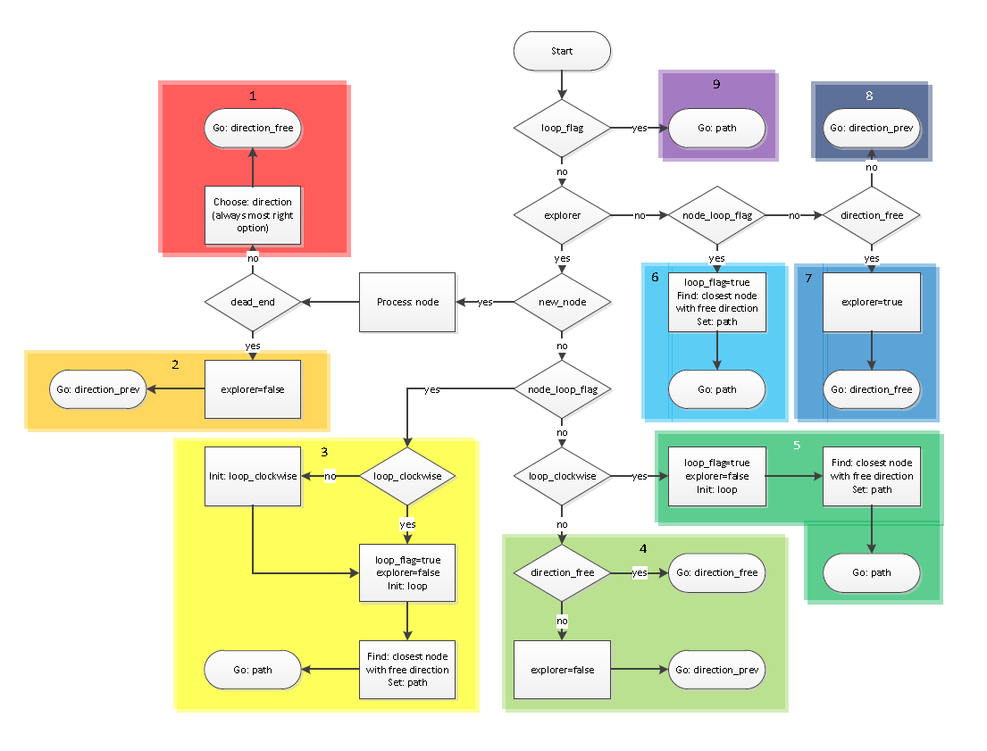
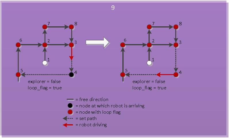
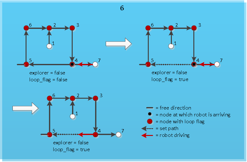
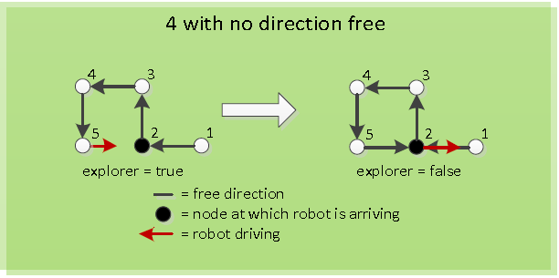
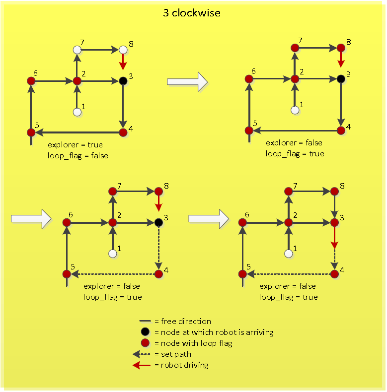
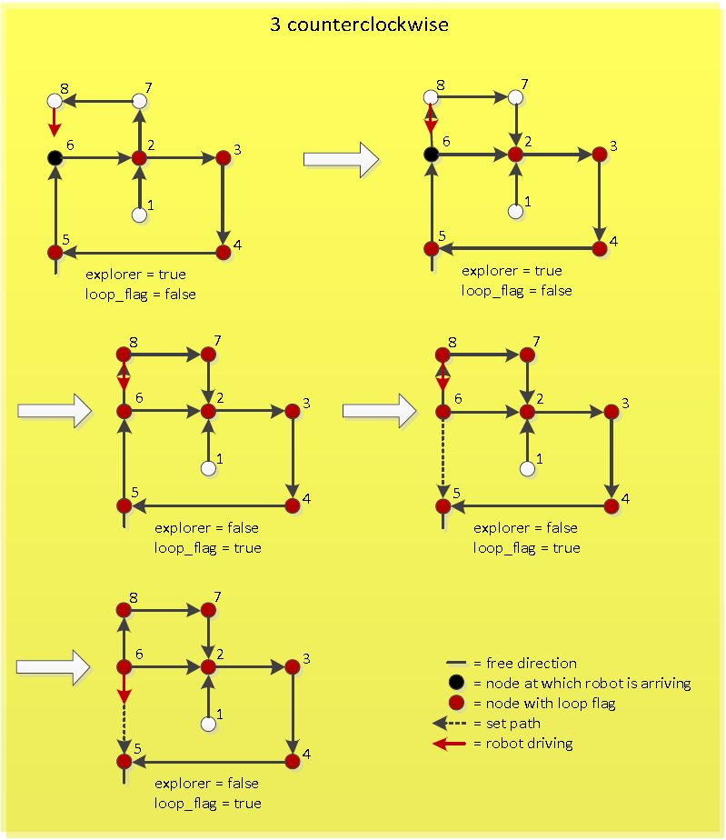
If the new loop has a counterclockwise direction, first the new loop has to be initialized clockwise. This means that the nodes in the new loop are set in a clockwise order. So the node at which the robot is just arriving now becomes the previous node of the node from which the robot just came. After this the same procedure can be followed as when the new loop is clockwise initially, because now the new counterclockwise loop is made a new clockwise loop. The working of this is visualized in Figure "Arriving at known node of counterclockwise loop". | If the new loop has a counterclockwise direction, first the new loop has to be initialized clockwise. This means that the nodes in the new loop are set in a clockwise order. So the node at which the robot is just arriving now becomes the previous node of the node from which the robot just came. After this the same procedure can be followed as when the new loop is clockwise initially, because now the new counterclockwise loop is made a new clockwise loop. The working of this is visualized in Figure "Arriving at known node of counterclockwise loop". | ||
</td><td>[[File:Pic_3_clockwise_algorithm.PNG|thumb|200px|''Arriving at known node of clockwise loop'']]</td><td>[[File:Pic_3_counterclockwise_algorithm.PNG|thumb|200px|''Arriving at known node of counterclockwise loop'']]</td></tr></table> | </td><td>[[File:Pic_3_clockwise_algorithm.PNG|thumb|200px|''Arriving at known node of clockwise loop'']]</td><td>[[File:Pic_3_counterclockwise_algorithm.PNG|thumb|200px|''Arriving at known node of counterclockwise loop'']]</td></tr></table> | ||
==Arrow detection== | |||
The arrow processing only is performed at T-crossings, since they are only useful at these crossings. The arrow processing algorithm is performed with the OpenCV package and is performed in several steps, which are given here: <br> | |||
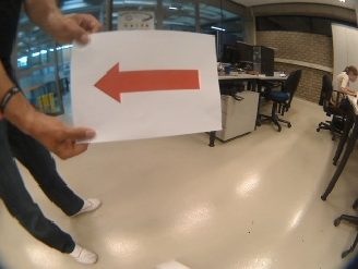
* First the camera image, which is shown in Figure “Camera Image” is converted into an HSV image. | |||
* The different channels (Hue, Saturation, Value) are split. | |||
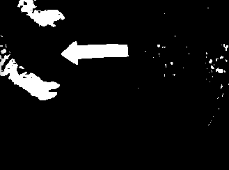
* The Hue and Saturation channels are thresholded with a lower and upper bound and the combination of these two channels are merged into 1 image, which is shown in Figure “Thresholded Image”. The lower and upper bound of the Hue channel are 100 and 150 respectively. The lower and upper bound of the Saturation channel are 100 and 210 respectively. | |||
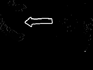
* After the thresholding, the image is dilated and eroded, to close possible gaps in the arrow. The image after closing is shown in Figure “Closed Image”. | |||
* The contours can be detected of this binary image using the findContours function in OpenCV. | |||
* Every contour is checked whether it is an arrow using four key points, namely the most left, bottom, right and top point. | |||
* The arrow is highlighted and shown in Figure “Arrow detected”. The direction is returned to the algorithm. | |||
<table> | |||
<tr> | |||
<td>[[File:Pic_img_1_original.png|200px|thumb|Figure "Camera Image"]]</td> | |||
<td>[[File:Pic_img_2_thresholded.png|200px|thumb|Figure "Thresholded Image"]]</td> | |||
<td>[[File:Pic_img_3_dilate_erode.png|200px|thumb|Figure "Closed Image"]]</td> | |||
<td>[[File:Pic_img_4_processed.png|200px|thumb|Figure "Arrow detected"]]</td> | |||
</tr> | |||
</table> | |||
==Simulation results== | |||
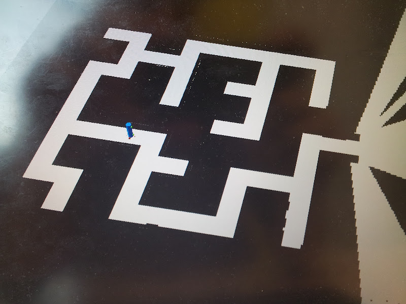
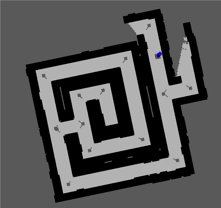
Managed to solve various mazes in simulation. Make sure you take a look at the fourth video, triple loop maze solved! | |||
Movies: | |||
<table> | |||
<tr> | |||
<td>[[File:Movie4_emc01.png|200px|thumb|http://www.youtube.com/watch?v=tgHOjsxDUjk&feature=plcp]]</td> | |||
<td>[[File:F1.PNG|200px|thumb|https://www.youtube.com/watch?v=e1CASyzed3E&feature=plcp]]</td> | |||
<td>[[File:F2.PNG|200px|thumb|https://www.youtube.com/watch?v=qrbDDAJchS8&feature=plcp]]</td> | |||
<td>[[File:F4.PNG|200px|thumb|https://www.youtube.com/watch?v=XwLcYULewZ8&feature=plcp]]</td> | |||
</tr> | |||
</table> | |||
==Experimental results== | |||
<table> | |||
<tr> | |||
<td>[[File:Test1.png|200px|thumb|http://youtu.be/_g9S24xXes4]]</td> | |||
<td>[[File:F3.PNG|200px|thumb|https://www.youtube.com/watch?v=HjW0VavlWrg&feature=plcp]]</td> | |||
</tr> | |||
</table> | |||
Latest revision as of 13:33, 26 June 2012
Group Members
| Name: | Student id: | Email: |
| Rein Appeldoorn | 0657407 | r.p.w.appeldoorn@student.tue.nl |
| Jeroen Graafmans | 0657171 | j.a.j.graafmans@student.tue.nl |
| Bart Peeters | 0748906 | b.p.j.j.peeters@student.tue.nl |
| Ton Peters | 0662103 | t.m.c.peters@student.tue.nl |
| Scott van Venrooij | 0658912 | s.j.p.v.venrooij@student.tue.nl |
Tutor: Jos Elfring
Progress
Week 1
- Installed all required software on our computers :)
- Everybody gained some knowledge about Unix, ROS and C++.
Week 2
|
 | |
Week 5
- Map-processing is cancelled, since the used package (hector_mapping) creates incorrect maps.
- Now working on processing the laserdata to let the Jazz drive "autonomously"
- Writing an algorithm by using depth-first-search, this algorithm obtains the kind of crossing, the position of the Robot and the angle of the Robot and sends the new direction to the Robot
Week 6
Tasks for Week 7:
|
 |
 | ||
Week 7
|
 |
 | ||
Week 8
|
 |
 | ||
Week 9
|
 |
 |
 | |
StrategyThe navigation node is used to steer the robot correctly in the maze. This navigating is done with use of the laser data. The laser data is first set into a certain variable. On the basis of this variable the robot can be navigated through the maze. The navigation is divided into 6 cases. The first case is the case in which the robot is driving trough a corridor. In this case the robot is kept in the middle of the corridor by checking and adjusting its angle with respect to the walls of the corridors. While driving trough it is constantly checked whether a corner of any type or a dead end can be recognized. Whenever a corner is recognized, the navigation switches to case 2. In case 2 the recognized corner or dead end is labeled as one of seven possible corner-types. This corner-type can be a corner left or right, one of three possible T-junctions, a cross-over or a dead end. These corner-types all get a number to identify them easily: In case 4 the robot makes a turn or does nothing. This is dependant of the direction in which the robot has to go. If the algorithm node publishes as direction to go straight ahead, the robot will not do anything in case 4 and will immediately switch to case 5. On the other hand, if the algorithm publishes to go to the left or right, the robot will make a turn of +(1/2)π radials or -(1/2)π radials respectively. After the turn is completed, the navigation switches to case 5. In case 5 the robot starts driving forward again until it reaches the corridor. When the corridor is reached, the navigation switches back to case 1. Case 6 is the case in which the navigation goes, when the robot is driving towards a dead end. In this case only direction is possible and that is backwards. So after driving to center of the dead end, which is at half the distance of a corridor of the dead end, the robot will make a turn of π radials. After the turn is completed, the navigation switches back to case 1. Detection corners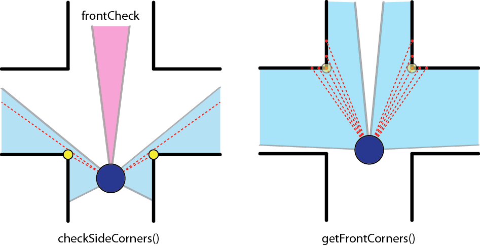 Determine CornerTypeIf the robot arrives at a crossing, a specific algorithm is triggered to determine the type of the crossing. The algorithm determines the cornerType which use of three variables (as can also be seen in the left figure):
Based on these three booleans, the cornerType can be determined using some logical operators. The pseudo code algorithm to detect the sideCorners is given below: loop over specific range of laser data points:
if we look at the left side:
if distance[i] > distance[i+1] AND distance[i]/distance[i+1] > ratioTreshold:
Do some extra checks
if extraChecks succeed then return true end
end
end
if we look at the right side:
if distance[i] < distance[i+1] AND distance[i]/distance[i+1] > ratioTreshold:
Do some extra checks
if extraChecks succeed then return true end
end
end
Find FrontCorners to determine reference PhiFinding these 90 degrees front corners is used in the following states:
The figure on the right illustrates the working of the detection method. In short, the algorithm iterates over a specif domain of laser-points. At each point, it checks the angle between the previous and following laserpoint around its vertical axis. If this angle is more or less 90 degrees, a 90 degrees angle has been found on the x,y position of the base. The algorithm in pseudocode is given below: loop over specific range of laser data points
Determine coordinates of each point relative to the robot
Base = coordinates[i]
Vector1 = coordinates[i-offset]-coordinates[i]
Vector2 = coordinates[i+offset]-coordinates[i]
Normalize vectors
innerProduct = innerProduct of vectors Vector1 and Vector2
if innerProduct is close to zero:
// Possible 90 degrees angle at coordinates[i]
Do some extra checks to make sure coordinates[i] is at a 90 degrees angle
if extra checks are true:
return the x and y value of the 90 degrees angle
end
end
return that no corner of 90 degrees is found
Controller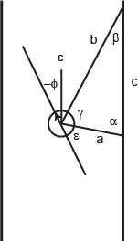 The forward velocity is set to a constant velocity (v = 0.1) under all circumstances, except when making a turn. AlgorithmArrow detectionThe arrow processing only is performed at T-crossings, since they are only useful at these crossings. The arrow processing algorithm is performed with the OpenCV package and is performed in several steps, which are given here:
Simulation resultsManaged to solve various mazes in simulation. Make sure you take a look at the fourth video, triple loop maze solved! Movies: Experimental results
|
|||||||
