Embedded Motion Control 2016 Group 4: Difference between revisions
| (116 intermediate revisions by 4 users not shown) | |||
| Line 27: | Line 27: | ||
[mailto:t.j.josten@student.tue.nl;t.c.p.f.leenen@student.tue.nl;m.plantinga@student.tue.nl;j.m.f.reinders@student.tue.nl Email all groupmembers] | [mailto:t.j.josten@student.tue.nl;t.c.p.f.leenen@student.tue.nl;m.plantinga@student.tue.nl;j.m.f.reinders@student.tue.nl Email all groupmembers] | ||
= '''Goal'' | = '''Initial design idea''' = | ||
== ''Goal'' == | |||
The goal of this project is to make a robot (PICO or TACO) navigate autonomously and as seamlessly as possible through a maze and find the exit. The robot has a computer integrated in it that runs on Linux, with ROS (Robot Operating System) running on top. The software has to | The goal of this project is to make a robot (PICO or TACO) navigate autonomously and as seamlessly as possible through a maze and find the exit. The robot has a computer integrated in it that runs on Linux, with ROS (Robot Operating System) running on top. The software has to | ||
be written in the C++ programming language. To achieve the goal, a software architecture has to be designed that structurally makes room for the different requirements, functions, components, specifications and interfaces. | be written in the C++ programming language. To achieve the goal, a software architecture has to be designed that structurally makes room for the different requirements, functions, components, specifications and interfaces. | ||
= | == ''Requirements'' == | ||
To achieve the final goal several requirements are determined, which can be seen in the following list. | To achieve the final goal several requirements are determined, which can be seen in the following list. | ||
| Line 55: | Line 57: | ||
:**''the software should be able to work independently of the size and structure of the maze'' | :**''the software should be able to work independently of the size and structure of the maze'' | ||
= | == ''Functions'' == | ||
The functions can be divided into two groups: the basic functions and the skill functions. The basic functions are basic actions that the robot will do. The skill functions are a set of actions to accomplish a certain goal. | The functions can be divided into two groups: the basic functions and the skill functions. The basic functions are basic actions that the robot will do. The skill functions are a set of actions to accomplish a certain goal. | ||
| Line 95: | Line 97: | ||
:**Input: current and expected x, y and theta of the robot; Output: new motion of the robot based upon the result. | :**Input: current and expected x, y and theta of the robot; Output: new motion of the robot based upon the result. | ||
= | == ''Components'' == | ||
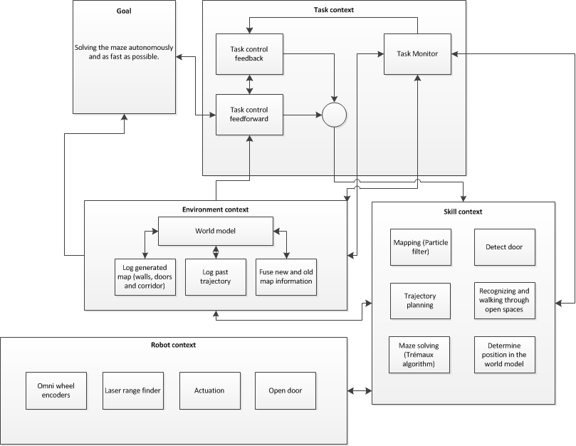
To fulfilll the previously mentioned functions and achieve the goal, the software should contain different components that interact with each other. This can be seen in Figure 1. | To fulfilll the previously mentioned functions and achieve the goal, the software should contain different components that interact with each other. This can be seen in Figure 1. | ||
| Line 111: | Line 113: | ||
[[File:PlaatjeFinal.png|thumb|center|1000px|Figure 1: Structure of the software implementation]] | [[File:PlaatjeFinal.png|thumb|center|1000px|Figure 1: Structure of the software implementation]] | ||
= | == ''Specifications'' == | ||
In the specifications the tasks that the robot has to conduct are quantified (i.e. given a value). | In the specifications the tasks that the robot has to conduct are quantified (i.e. given a value). | ||
| Line 120: | Line 122: | ||
:* PICO may not stop moving for more than 30 seconds (e.g. when opening the door) | :* PICO may not stop moving for more than 30 seconds (e.g. when opening the door) | ||
== ''Interfaces'' == | |||
= | |||
To interpret the data that the robot collects, it is convenient to make a graphical user interface that visualizes this data. The omni-wheel encoder in combination with the laser range finder can | To interpret the data that the robot collects, it is convenient to make a graphical user interface that visualizes this data. The omni-wheel encoder in combination with the laser range finder can | ||
| Line 128: | Line 129: | ||
The laser range finder also produces data, and to see if this data is interpreted in the right way a visualization should be made. It can be used to see if walls, doors and exits are detected in the | The laser range finder also produces data, and to see if this data is interpreted in the right way a visualization should be made. It can be used to see if walls, doors and exits are detected in the | ||
right way. Possible algorithms for this are the Hough transform and particle filter. | right way. Possible algorithms for this are the Hough transform and particle filter. | ||
= '''Corridor Challenge''' = | = '''Corridor Challenge''' = | ||
The goal of the corridor challenge | The goal of the corridor challenge is to let Pico take the first exit, either left or right, out of a corridor. | ||
It is decided to let Pico drive forward and use its potential force field to keep him in the middle of the corridor (The potential field is more comprehensively discussed under the section potential field). At the moment when Pico sees the exit, he should turn 90 degrees in the direction where the exit is and then continue with driving forward and use the potential force field. A animation is shown in the figure below. | It is decided to let Pico drive forward and use its potential force field to keep him in the middle of the corridor (The potential field is more comprehensively discussed under the section potential field). At the moment when Pico sees the exit, he should turn 90 degrees in the direction where the exit is and then continue with driving forward and use the potential force field. A animation is shown in the figure below. | ||
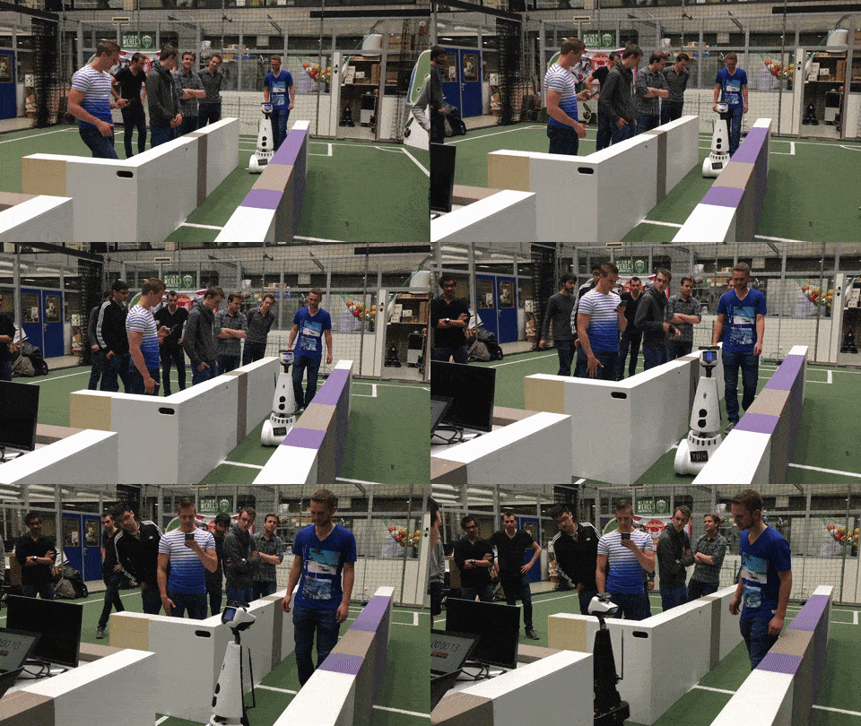
[[File:GifCorridor.gif|thumb|center|500px|Figure | [[File:GifCorridor.gif|thumb|center|500px|Figure 2: Overview of the steps to solve the corridor challenge]] | ||
Although it would have been better and quicker to detect the exit before it is next to pico and then put a setpoint (point of attraction for the force field) at the exit. Because, this way Pico does not have to come to a complete stop and keeps driving. But because the potential field was well tuned it was possible to drive very fast which made us finish the corridor challenge the fastest. The video of our second run is shown below. | Although it would have been better and quicker to detect the exit before it is next to pico and then put a setpoint (point of attraction for the force field) at the exit. Because, this way Pico does not have to come to a complete stop and keeps driving. But because the potential field was well tuned it was possible to drive very fast which made us finish the corridor challenge in the fastest time. The video of our second run is shown below. | ||
[[File:Corridor_movie.gif|thumb|center|1000px|Figure 3: Solving the corridor challenge]] | |||
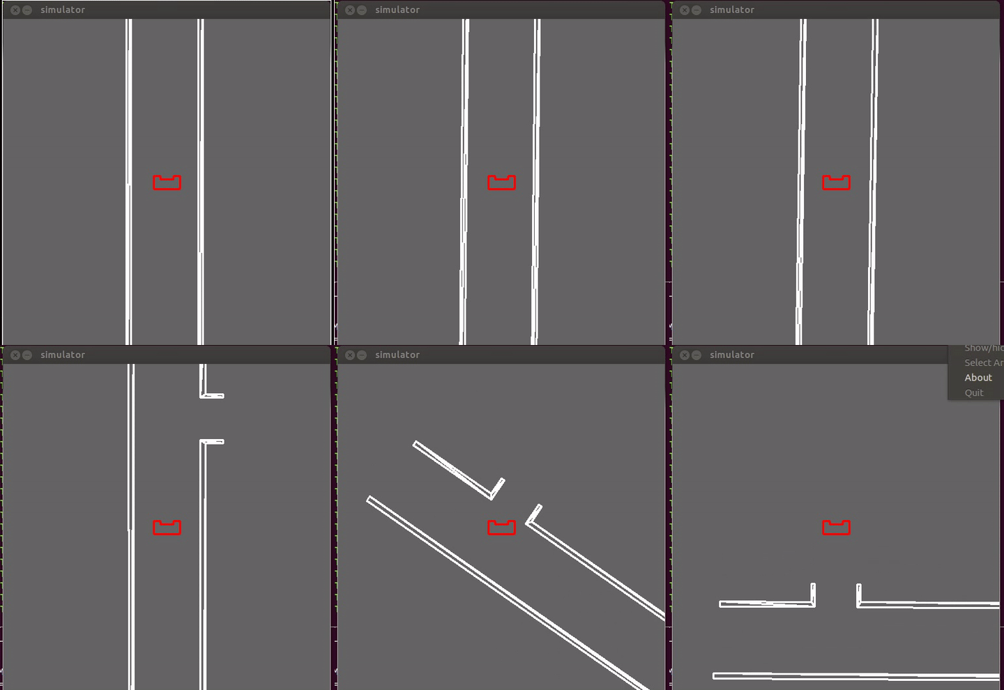
Finally, the script is adjusted such that it uses node detection and it makes nice smooth turns, a video of this in the simulator is shown in Figure 4. | |||
[[File:Corridor_Tom.gif|thumb|center|1000px|Figure 4: Corridor challenge in the simulator]] | |||
= '''Maze Challenge''' = | = '''Maze Challenge''' = | ||
| Line 143: | Line 151: | ||
= ''Software architecture & approach'' = | = ''Software architecture & approach'' = | ||
To make a good code first of all the software architecture is obtained. This is visually displayed in Figure 5. First of all data is obtained from Pico, this is done using the two sensors, the laser range finder and odometry. The laser range finder data is used to generate a potential field and to discover features (nodes) furthermore there is the odometry data, which is used to determine an initial guess for the position for the mapping block. Features (e.g. T-junction, dead end or corners) are detected using the node detection algorithm as described in the next part. Using these features and the odometry data a map is generated. The information in this map is used by the target to determine what step to take (i.e. open door, turn or drive). This target is combined with the potential field and is used to make Pico drive in the desired direction. | |||
[[File:Chart-eps-converted-to-1_g4.png|thumb|center|700px|Figure | [[File:Chart-eps-converted-to-1_g4.png|thumb|center|700px|Figure 5: Software architecture]] | ||
= '' | = ''Node detection (Features)'' = | ||
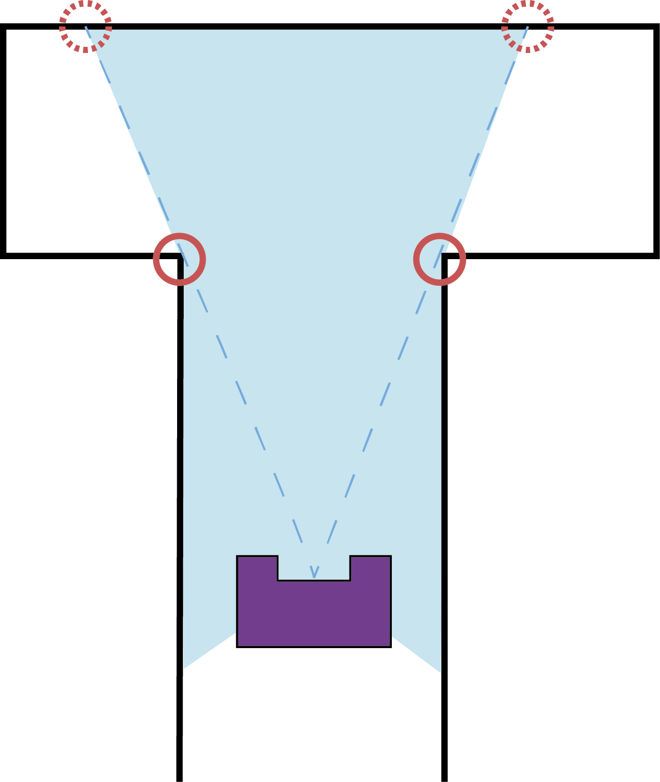
To drive through the maze correctly, locally nodes (e.g. T-junction or crossroads) have to be detected. In order to do this, features from the environment have to be detected. As the world in which PICO lives consists of straight walls, detecting the vertices of the walls (as seen from above) is a good choice. Certain vertices can be distinguished in a relatively simple manner by looking at how the LRF data jumps abruptly from one measurement to the other. An example of such a situation can be seen in Figure 6, here the circles indicate how from one measurement to another there is a large jump. By determining the distance between consecutive measurement points, if a certain threshold value is exceeded it's an indicative of a vertex. The threshold value is a magic number, but given the fact that the minimum width between walls is know (i.e. 0.5 m), a good estimation of a suitable value can be made. | |||
The question however is where the vertex is placed. From Figure 6 it is clear that the vertices should be placed at the position of the non-dotted circles. But how can this be translated to the computer? Analyzing this and similar other scenarios leads to the conclusion that the vertex will always be the one that lies closest to PICO. The dotted circles are ghost vertices. | |||
[[File:Virtual vertices.png|thumb|center|250px|Figure 6: Vertices and ghost vertices]] | |||
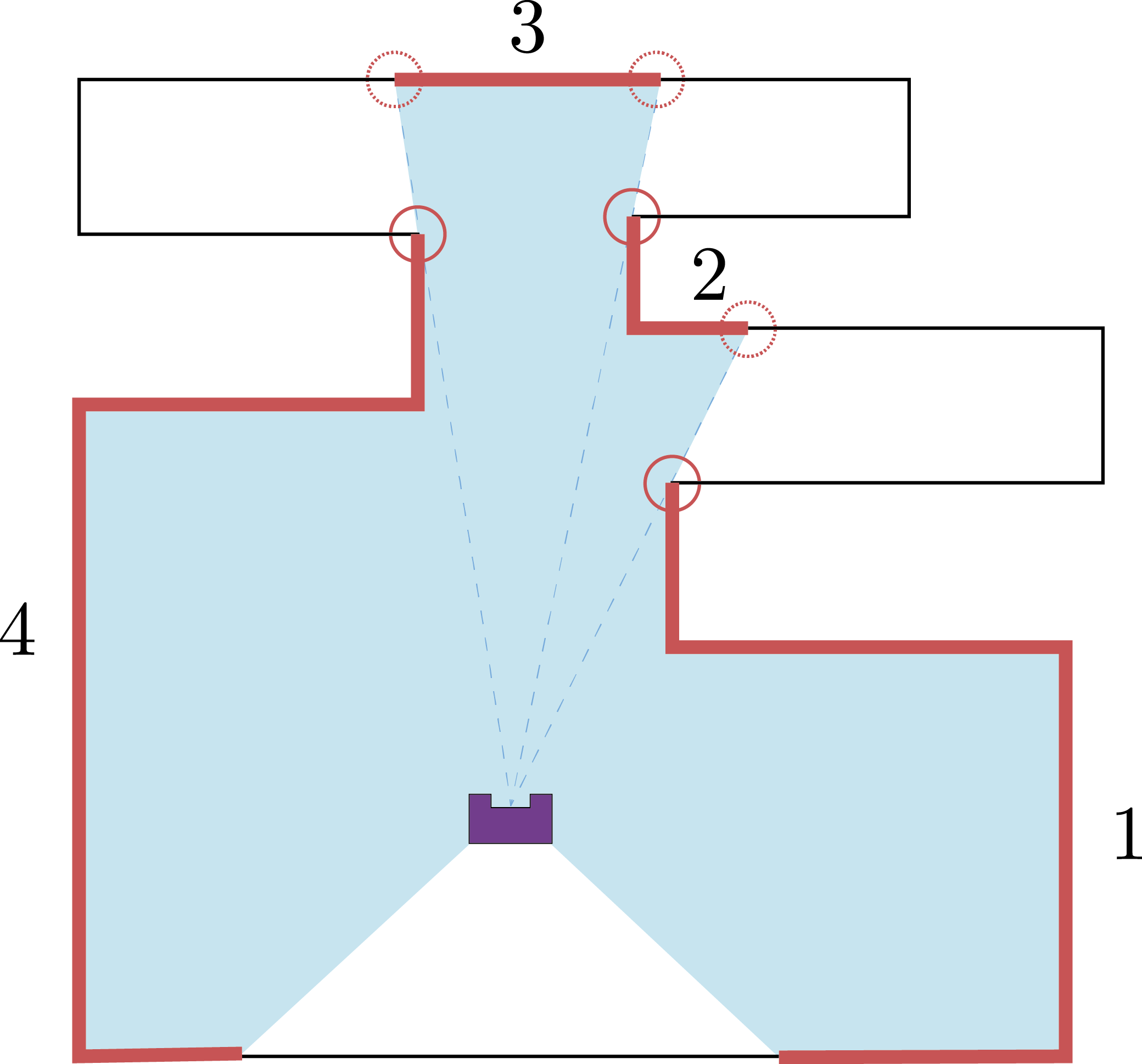
Given that the vertices have been found, the measurement data can be separated into three different segments. Figure 7 displays a more involved scenario. Again ghost vertices are marked by dotted circles and real vertices are marked by normal circles. There are four different segments that can be distinguished based on the vertices. These are indicated by their corresponding number. What immediately becomes clear from this figure is that not all the vertices are found. Within the different segments there are various vertices that can not be found by means of the method described above. In order to find these vertices a Split-and-Merge algorithm can be used. | |||
[[File:Virtual vertices2.png|thumb|center|400px|Figure 7: Segmentation from vertices]] | |||
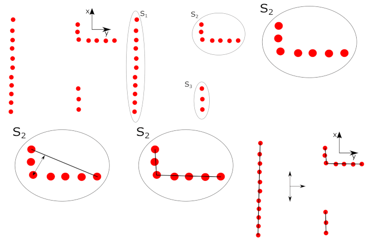
The Split-and-Merge algorithm works as follows (A visualization is shown in Figure 8): | |||
#For each of the segments a virtual line is determined that connects the begin and end points of the segment | |||
#Within each segment, the maximum distance between the measurement points of the segment and the virtual line is determined. | |||
#If the above maximum distance is above a threshold (e.g. 0.2m), the corresponding measurement point is considered a vertex within the segment | |||
#The above is repeated for all segments until no new vertices are found | |||
#Once all vertices are found, straight lines between the different vertices are defined | |||
[[File:GIF_joey_g4.gif|thumb|center|250px|Figure 8: Node detection]] | |||
In order to implement this into code, C++ Standard Library (stl) vectors of structs are used. Two different structs are defined, one for vertices and one for edges. When new vertices are found these are placed in a vector or Vertex structs. Similarly when new edges are found, these are placed in a vector of Edges structs. This gives the freedom to easily add or delete vertices, independent of the amount or position. | |||
<nowiki> struct Vertex | |||
{ | |||
double x; | |||
double y; | |||
double angle; | |||
double range; | |||
int id; | |||
}; | |||
struct Edges | |||
{ | |||
int id_begin; | |||
int id_end; | |||
Coordinates pt_begin; | |||
Coordinates pt_end; | |||
Edges (int id1, int id2, Coordinates pt1, Coordinates pt2) | |||
: id_begin(id1), id_end(id2), pt_begin(pt1), pt_end(pt2){} | |||
}; | |||
</nowiki> | |||
Using the lines as extracted with the algorithm described above a distinction is made in walls aligned with pico and walls which are orthogonal to pico. Based on the walls which are aligned with pico and the distance in x direction between those wall it is determined if it is possible to go right or left. | Using the lines as extracted with the algorithm described above a distinction is made in walls aligned with pico and walls which are orthogonal to pico. Based on the walls which are aligned with pico and the distance in x direction between those wall it is determined if it is possible to go right or left. | ||
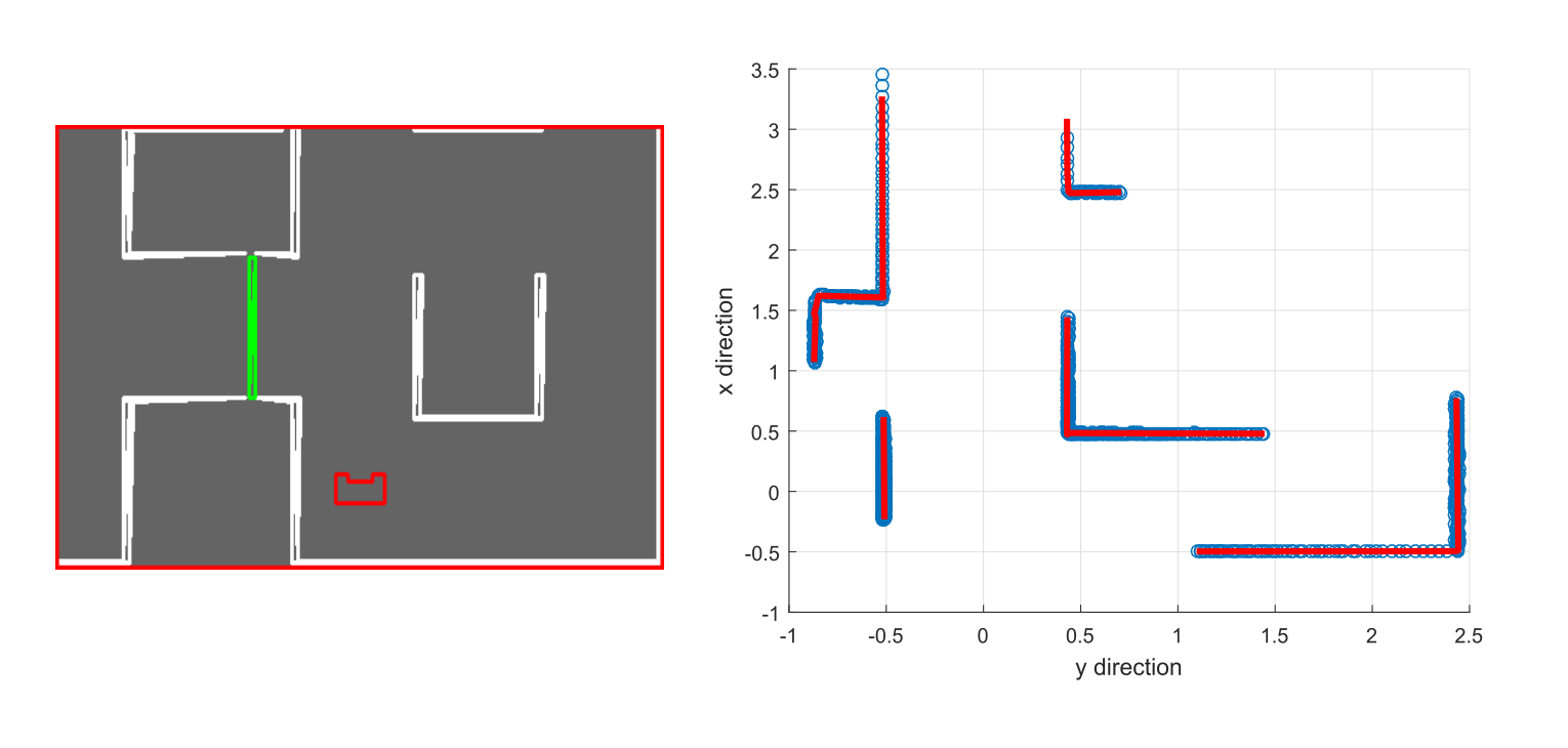
An example of the fitted walls using the simulator is shown in Figure | An example of the fitted walls using the simulator is shown in Figure 9, with in the right part the LRF data and the fitted lines, and in the left part what the simulator shows. This clearly shows that all the walls of the simulation (up to the specified distance to see) are extracted nicely. Based on these lines the nodes (crossings) are positioned in local coordinates. | ||
[[File:NodeExtractionExample.png|thumb|center|1000px|Figure 9: Example of the node detection in the simulator for the final maze.]] | |||
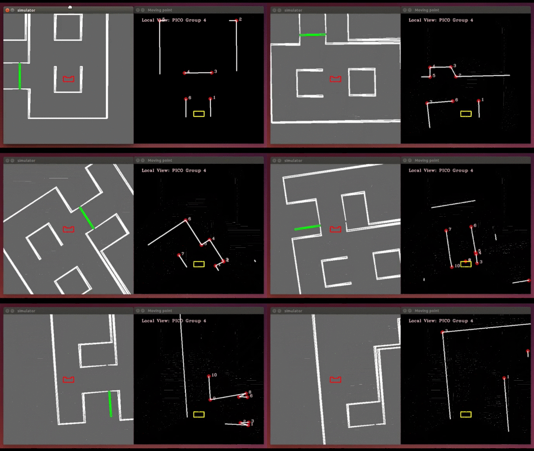
[[File: | Below a visualization is shown of Pico driving through the final maze. The visualization shows the walls and the obtained corners which are used as features for the kalman filter. | ||
[[File:EMC.gif|thumb|center|750px|Figure 10: Visualization of the line extraction while driving in the maze of the final challenge.]] | |||
The code that is used to obtain the different vertices and edges can be found below: | |||
https://gitlab.com/emc2016/group4/blob/wiki_code/EKF/src/nr.cpp | |||
https://gitlab.com/emc2016/group4/blob/wiki_code/EKF/src/nr.hpp | |||
https://gitlab.com/emc2016/group4/blob/wiki_code/EKF/src/viz.hpp | |||
The main script is nr.cpp, which uses the header files nr.hpp and viz.hpp for functions and visualization. | |||
= ''SLAM (Simultaneous localization and mapping)'' = | = ''SLAM (Simultaneous localization and mapping)'' = | ||
To estimate the location of Pico and to get a map of the maze, the SLAM algorithm is used. First some definitions are | To estimate the location of Pico and to get a map of the maze, the SLAM algorithm is used. An extended Kalman filter is used in this algorithm, which will be described below. | ||
First some definitions are given. | |||
=== '''Definitions''' === | === '''Definitions''' === | ||
| Line 182: | Line 238: | ||
# <math> k </math>: time step. | # <math> k </math>: time step. | ||
=== '''Association of points between measurements''' === | |||
In order to be able to apply the extended Kalman filter, if in between measurements a feature is seen again it has to be detected as the same feature and not a new one. In order to make sure this happens for all viewed features these have to be passed through an association algorithm. The below link shows the association algorithm that is applied: | |||
https://gitlab.com/emc2016/group4/blob/wiki_code/EKF/src/c2f_function.cpp | |||
The script in the link is a function that takes in the vertices that where found during node recognition. When the vertices are sent for a second time to c2f_function.cpp, the algorithm looks if the vertices that have been sent are within a certain ball with respect to the vertices that were sent the first time. If a vertex is seen again, the vertex is seen as persistent over time. Similarly, if the vertex is not seen for a while the vertex is seen as non-persistent. This way, by doing bookkeeping on how often a vertex is seen, it can be either added or deleted from a list of structs containing features. Adding it to or deleting a feature from the list of structures depend on if the feature has been seen for more than or les than a certain amount of times, respectively. The list of structures can then be returned to the main script allowing to see how features process over measurements. | |||
=== '''Position estimation and equations of motion''' === | === '''Position estimation and equations of motion''' === | ||
To estimate the position of Pico, odometry data is used. And since the frequency is high, the motions are relatively small and it is assumed that: <math>\delta_d= \delta_s</math> which can be seen in Figure | To estimate the position of Pico, odometry data is used. And since the frequency is high, the motions are relatively small and it is assumed that: <math>\delta_d= \delta_s</math> which can be seen in Figure 11. | ||
[[File:Plaatjeddds-1.png|thumb|center| | [[File:Plaatjeddds-1.png|thumb|center|400px|Figure 11: Position estimation]] | ||
<ul> | <ul> | ||
| Line 268: | Line 331: | ||
=== '''Extended Kalman Filter''' === | === '''Extended Kalman Filter''' === | ||
Given noisy odometry data, how can we estimate new pose given previous pose and noisy odometry? Kalman filter provides optimal estimate of the system state assuming zero mean Gaussian noise. | |||
: | The used motion model is a non-linear model. Therefore the motion model is locally linearized wrt the current state estimate <math> \hat{x}_{{\langle k \rangle}}</math>, resulting in <br> | ||
::<math>\hat{x}_{{\langle k+1 | k+1 \rangle}}= \hat{x}_{{\langle k+1 | k \rangle}}+ K_{{\langle k+1 \rangle}}\nu_{{\langle k+1 \rangle}}</math | ::<math>\hat{x}_{{\langle k+1 \rangle}}= \hat{x}_{{\langle k \rangle}}+ F_x(x_{{\langle k \rangle}}- \hat{x}_{{\langle k \rangle}}) + F_v v_{{\langle k \rangle}},</math> | ||
<br> | |||
where <math> F_x = \frac{\partial f}{\partial x} </math> and <math> F_v = \frac{\partial f}{\partial v} </math> are Jacobians. These are obtained by differentiating and evaluating for <math> v = 0 </math>: | |||
<br> | |||
::<math>F_x = \left.\frac{\partial f}{\partial x}\right|_{v=0} = \begin{bmatrix} | |||
1 & 0 &-\delta_{d,{{\langle k \rangle}}} - \sin(\theta_{{\langle k \rangle}}+ \delta_\theta)\\ | |||
0&1&\delta_{d,{{\langle k \rangle}}}\cos(\theta_{{\langle k \rangle}}+ \delta_\theta)\\ | |||
0&0&1 | |||
\end{bmatrix}</math> | |||
<br> | |||
::<math>F_v = \left.\frac{\partial f}{\partial v}\right|_{v=0} = \begin{bmatrix} | |||
\cos(\theta_{{\langle k \rangle}}+\delta_\theta) &-\delta_{d,{{\langle k \rangle}}}\sin(\theta_{{\langle k \rangle}}+ \delta_\theta)\\ | |||
\sin(\theta_{{\langle k \rangle}}+\delta_\theta)&\delta_{d,{{\langle k \rangle}}}\cos(\theta_{{\langle k \rangle}}+ \delta_\theta)\\ | |||
0&1 | |||
\end{bmatrix}</math> | |||
==== '''Preliminaries''' ==== | |||
# Define the initial state covariance <math> P_0 </math>.<br /> The values of the elements of this matrix can be small given that a good initial state estimation is assumed. | |||
# Define the estimate of the odometry covariance (<math> V </math>) <math>, \hat{V} </math>.<br /> Some experimentation is required to determine an appropriate value of <math> \hat{V} </math>. | |||
# Determine the estimated LRF covariance <math> \hat{W} </math> | |||
==== '''Steps''' ==== | |||
The steps are as follows: | |||
# EKF Prediction Equations | |||
<br> | |||
::<math>\hat{x}_{\langle k+1 | k\rangle} = f(\hat{x}_{\langle k\rangle}, \delta_{\langle k \rangle}, 0)</math> | |||
<br> | |||
::<math>\hat{P}_{{{\langle k+1 | k \rangle}}} = F_{x, \langle k \rangle}\hat{P}_{{\langle k | k \rangle}}F_{x, \langle k \rangle}{^\top}+ F_{v, \langle k \rangle }\hat{V} F_{v, \langle k \rangle}{^\top}</math> | |||
# EKF Sensor Update Equations <math>\hat{x}_{{\langle k+1 | k+1 \rangle}}= \hat{x}_{{\langle k+1 | k \rangle}}+ K_{{\langle k+1 \rangle}}\nu_{{\langle k+1 \rangle}}</math><math>\hat{P}_{{\langle k+1 | k+1 \rangle}}= \hat{P}_{{\langle k+1 | k \rangle}}F_{x,{{\langle k \rangle}}}{^\top}- K_{{\langle k+1 \rangle}}H_{x,{{\langle k+1 \rangle}}}\hat{P}_{{\langle k+1 | k \rangle}}</math><math>S_{{\langle k+1 \rangle}}= H_{x,{{\langle k+1 \rangle}}} \hat{P}_{{\langle k+1 | k \rangle}}H_{x,{{\langle k+1 \rangle}}}{^\top}+ H_{w,{{\langle k+1 \rangle}}}\hat{W}_{{\langle k+1 \rangle}}H_{w,{{\langle k+1 \rangle}}}{^\top}</math><math>K_{{\langle k+1 \rangle}}= \hat{P}_{{\langle k+1 | k \rangle}}H_{x,{{\langle k+1 \rangle}}}{^\top}S_{{\langle k+1 \rangle}}{^{-1} }</math> | |||
==== '''Sensor Fusion''' ==== | |||
The EKF framework allows data from many and varied sensors to update the state. This is the reason the estimation problem is also referred to as sensor fusion. Compass heading angle, GPS position, gyroscope yaw rate and target bearing angle can be all used to update the state. | |||
All that is needed is | |||
# Observation function <math> h(.) </math> | |||
# Jacobians <math> H_x </math> and <math> H_w </math> | |||
# Estimate of sensor output covariance <math> W </math> | |||
The observation function <math> h(.) </math> can be both non-linear and non-invertible, the EKF does the rest. | |||
=== '''Map Making''' === | === '''Map Making''' === | ||
<ul> | <ul> | ||
<p>The state vector with estimated coordinates to <math> m </math> landmarks can be described as | |||
<br> | <br> | ||
::<math>\hat{x}=(x_1, y_1,\dots, x_m, y_m){^\top}</math></p></li> | ::<math>\hat{x}=(x_1, y_1,\dots, x_m, y_m){^\top}</math></p></li> | ||
<li><p> | <li><p>Now the prediction equations are as follows | ||
<br> | <br> | ||
::<math>\hat{x}_{{\langle k+1 | k \rangle}}= \hat{x}_{{\langle k | k \rangle}}</math> | ::<math>\hat{x}_{{\langle k+1 | k \rangle}}= \hat{x}_{{\langle k | k \rangle}}</math> | ||
::<math>\hat{P}_{{\langle k+1 | k \rangle}}= \hat{P}_{{\langle k | k \rangle}}</math></p></li> | ::<math>\hat{P}_{{\langle k+1 | k \rangle}}= \hat{P}_{{\langle k | k \rangle}}</math></p></li> | ||
<li><p> | <li><p>With the state vector evolution</p> | ||
::<p><math>g(x_v,z) = | ::<p><math>g(x_v,z) = | ||
\begin{bmatrix} | \begin{bmatrix} | ||
| Line 290: | Line 395: | ||
y_v + r_z\sin(\theta_v + \theta_z) | y_v + r_z\sin(\theta_v + \theta_z) | ||
\end{bmatrix}</math></p></li> | \end{bmatrix}</math></p></li> | ||
<li><p>Adding landmarks | <li><p>Adding landmarks can be done according to | ||
<br> | <br> | ||
::<math>x_{{\langle k | k \rangle}}^\star | ::<math>x_{{\langle k | k \rangle}}^\star | ||
| Line 304: | Line 409: | ||
=== '''Simultaneous Localization and Mapping''' === | === '''Simultaneous Localization and Mapping''' === | ||
The state vector consists of both the pose as the coordinates of the <math> M </math> landmarks that have been seen thus far: | |||
<br> | |||
::<math>\hat{x} = (x_v, y_v, \theta_v, x_1, y_1, ... , x_m, y_m)</math> | ::<math>\hat{x} = (x_v, y_v, \theta_v, x_1, y_1, ... , x_m, y_m)</math> | ||
The covariance matrix is given by: | |||
::<math> | <br> | ||
::<math>\hat{P} | |||
= \begin{bmatrix} | |||
\hat{P_{vv}} &\hat{P}_{vm}\\ | |||
\hat{P}_{vm}{^\top}&\hat{P_{mm}} | |||
\end{bmatrix}</math> | |||
= ''Global and local path planning (Target and drive)'' = | When a new feature is observed, the state vector is updated, where <math> G_x </math> is now non-zero and given by: | ||
<br> | |||
::<math>G_x = \frac{\partial g}{\partial x_v} | |||
= | |||
\begin{bmatrix} | |||
1 &0 &-r_z\sin(\theta_v + \theta_z)\\ | |||
0 &1 &r_z\cos(\theta_v + \theta_z) | |||
\end{bmatrix}</math> | |||
as the estimate of the new feature depends on the state vector, which now contains the robot’s pose. | |||
Feature observation changes wrt the state vector are described by the Jacobian <math> H_x </math>. The observation depends on: | |||
# robot position | |||
# position of observed feature | |||
::<math>H_x = \left(H_{x_v} \dots 0 \dots H_{x_i} \dots 0\right),</math> | |||
where <math> H_{x_i} </math> is at the location corresponding to <math> x_i </math>. <math> H_{x_v} </math> has been added at the beginning to account for the position of the robot. | |||
= ''Global and local path planning (Target, potential field and drive)'' = | |||
=== '''Maze solving''' === | === '''Maze solving''' === | ||
| Line 324: | Line 454: | ||
</math> | </math> | ||
with <math>F_i</math> the force acting on Pico due to the point <math>i</math> and <math>r_i</math> the distance between Pico and the point <math>i</math>. Using the summation of all these forces gives a force in the x and y direction which are used to determine a x, y and rotational velocity. | with <math>F_i</math> the force acting on Pico due to the point <math>i</math> and <math>r_i</math> the distance between Pico and the point <math>i</math>. Using the summation of all these forces gives a force in the x and y direction which are used to determine a x, y and rotational velocity. To get a nice balance between these speed gain have been tuned for these speed during tests for different widths of corridors. | ||
To take turns using the potential field a force of attraction is used as shown in Figure | To take turns using the potential field a force of attraction is used as shown in Figure 12. This force is added to the repelling forces from the walls and thus pico will drive towards this point. | ||
Furthermore the potential field is used as collision avoidance as well. Because when it is implemented in a good way it is impossible to drive into the wall when it is active. | Furthermore the potential field is used as collision avoidance as well. Because when it is implemented in a good way it is impossible to drive into the wall when it is active. | ||
| Line 332: | Line 462: | ||
[[File:FORCEFIELD-1.png|thumb|center| | [[File:FORCEFIELD-1.png|thumb|center|350px|Figure 12: Potential field as used to drive through the maze]] | ||
= '''The final maze challenge''' = | |||
The 9th of June was the date of the maze challenge. In the link below a video is shown of our attempt at the maze challenge. As shown Pico does drive out of the maze but it is not in a very nice way. At the beginning it drives towards the wall which is ahead of him, this happens because Pico does not recognize the nodes in the right way. Due to the potential field it does not drive into the wall and slowly rotates and keeps driving around in the maze. At about 55 seconds it stands in the doorway and after some time it recognizes it and opens the door. But because Pico is not orientated with his front to the door it does not see that in front of him the distance becomes larger and thus it recognizes it as a dead end and turns around. Then Pico starts driving on its potential field again and finally at around 1:50 it reaches the openspace again and on just its potential field with a force in the x direction it reaches the exit in a little over 2 minutes. | |||
The YouTube video of the solved maze challenge can be found here: [https://youtu.be/xbM17MN8vyc The maze challenge solved] | |||
Based on this result it is concluded that the node recognition is not working good enough, therefore some adjustments are made and implemented in the simulator. A simulation on the same maze is conducted. As shown in the video in the link below the maze is successfully solved in simulations as well. | |||
The YouTube video of the solved maze in the simulator can be found here: [https://youtu.be/GkZij51VO3Y The maze challenge solved in the simulator] | |||
= '''Conclusions and recommendations''' = | = '''Conclusions and recommendations''' = | ||
== ''Conclusions'' == | |||
First of all it can be concluded that both goals are achieved, the corridor and the maze challenge are solved. | |||
Furthermore some conclusions are drawn about the progress of the project. During the project we encountered some problems, the first problem was the lack of experience in C++. No one in the group had experience in programming C++, this required some time in the beginning of the project. Then during the corridor challenge the result was good, but the problem with the code that was used, that most of it was not reusable for the maze challenge. Since for the maze challenge it is not just take a turn right or left, which was the only thing that in the corridor challenge which was detected. The part that is used for the maze challenge is the potential field, which worked very well. | |||
Then for the maze challenge some new problems occurred. The most important problem occurred due to the fact that the code became much bigger. It was hard to keep the code structured and to merge different parts of code, because multiple people where working on the code sometimes it became hard to understand every part of it. | |||
Another important lesson learned is to write the code in such a way that it is easy scalable and reusable for similar problems, this is done by making the "magic number" clear and understandable. | |||
Another problem occurred while testing, because the LRF showed some points in the real setup which were not there and thus had to be filtered out. Furthermore it must be able to work with gaps between walls. Also the tuning of the potential field had to be done for both the simulator as the real setup, because values that worked in the simulator did not make Pico drive smooth in reality. | |||
Furthermore it would have been helpful if we had one more group member, because the study load was more then 5 ECTS. | |||
== ''Recommendations'' == | |||
For future projects some recommendations are done. The first recommendation is that in the future a more structured approach should be used. Because the code becomes quite large it is important to make a clear overview of what function does what. Furthermore it is important to make more clear agreements within the group about what every function does (what does it get from other functions and what should it produce). Also it is important to start more easy. For example the SLAM algorithm which was immediately written with extended kalman filter etc. Maybe a more straightforward approach would have been better to start with. | |||
= '''Documents''' = | = '''Documents''' = | ||
Latest revision as of 01:01, 20 June 2016
Group Members
| ID-Number | Name | |
| 0811028 | Tim Josten | t.j.josten@student.tue.nl |
| 0790737 | Tom Leenen | t.c.p.f.leenen@student.tue.nl |
| 0832751 | Martin Plantinga | m.plantinga@student.tue.nl |
| 0816951 | Joey Reinders | j.m.f.reinders@student.tue.nl |
Initial design idea
Goal
The goal of this project is to make a robot (PICO or TACO) navigate autonomously and as seamlessly as possible through a maze and find the exit. The robot has a computer integrated in it that runs on Linux, with ROS (Robot Operating System) running on top. The software has to be written in the C++ programming language. To achieve the goal, a software architecture has to be designed that structurally makes room for the different requirements, functions, components, specifications and interfaces.
Requirements
To achieve the final goal several requirements are determined, which can be seen in the following list.
- Navigate autonomously to the exit of the maze as fast as possible
- cruise as fast as possible while maintaining the different abilities
- Navigate autonomously to the exit of the maze as fast as possible
- Avoid obstacles
- recognize the different obstacles (e.g. walls) and keep a "safe" distance from them
- Avoid obstacles
- Avoid getting trapped in a loop of the maze
- recognize if the robot is navigating through the same path over and over and exit the loop
- Avoid getting trapped in a loop of the maze
- Create a map of the maze
- Recognize door, open it and drive through it
- Navigate in open spaces
- navigate if no obstacle is in sight
- Navigate in open spaces
- Scalable system
- the software should be able to work independently of the size and structure of the maze
- Scalable system
Functions
The functions can be divided into two groups: the basic functions and the skill functions. The basic functions are basic actions that the robot will do. The skill functions are a set of actions to accomplish a certain goal.
The basic functions consist of:
- Actuation of the robot:
- Provide signals to the actuators of the robot. Realize the desired motion by using a controller and meeting the requirements.
- Input: location of robot, Output: motion of robot
- Actuation of the robot:
- Detect:
- Characterize different types of corridors based on telemetry provided by the Laser Range Finder (LRF).
- Input: measured x, y and theta; Output: type of corridor
- Detect:
The skill functions consist of:
- Mapping:
- Create and update a map of the explored maze. The robot will recall this map as its future moves will depend on this map.
- Input: current x, y and theta of the robot; Output: new/updated maze map, new/adjusted objective of the robot.
- Mapping:
- Feedback:
- Check position of robot with position of the created map. Prevent the robot from collisions with the walls or other obstacles.
- Input: current x, y, theta, LFR data and objective; Output: motion of the robot.
- Feedback:
- Decision:
- Check position of robot with position of the created map. Prevent the robot from collisions with the walls or other obstacles.
- Input: current x, y, theta, LFR data and objective; Output: motion of the robot
- Decision:
- Monitor:
- Control the exploration of the maze and prevent the robot from getting stuck in a loop.
- Input: current x, y and theta of the robot; Output: previously unexplored area
- Monitor:
- Door check:
- Wait at the potential door location for a predetermined time period while scanning the distance to the potential door to check if it opens.
- Input: current x, y and theta of the robot; Output: A door that either opens or stays closed, followed by pico's new objective based upon the result.
- Door check:
- Obstacle check:
- Measure the preset minimum safe distance from the walls or measure not moving as expected according to the driving action.
- Input: current and expected x, y and theta of the robot; Output: new motion of the robot based upon the result.
- Obstacle check:
Components
To fulfilll the previously mentioned functions and achieve the goal, the software should contain different components that interact with each other. This can be seen in Figure 1.
The C++ code should contain the components shown in Figure 1. There should be a task manager to switch between different tasks. An algorithm should be made that decides which task is performed or whether different tasks are performed simultaneously.
An algorithm should be implemented for controlling the robot and accurately position it, this algorithm uses the environment model, which is made using the laser range finder and omni-wheel encoders. This world model is logged and will be continuously updated during the maze solving of the robot.
The robot should have several skills and these should be programmed effectively with a fast algorithm. For the world model, the robot needs a mapping skill and it needs to determine its position in this world model. To solve the maze the robot needs a trajectory planning which uses an effcient maze solving algorithm (e.g. Trémaux).
Eventually when the robot has solved the maze, the algorithm has to be stopped.
Specifications
In the specifications the tasks that the robot has to conduct are quantified (i.e. given a value).
- The maximal translational velocity of PICO is 0.5 m/s
- The maximal rotational speed of PICO is 1.2 rad/s
- PICO has to solve the corridor challenge within 5 minutes
- PICO has to solve the maze challenge within 7 minutes
- PICO may not stop moving for more than 30 seconds (e.g. when opening the door)
Interfaces
To interpret the data that the robot collects, it is convenient to make a graphical user interface that visualizes this data. The omni-wheel encoder in combination with the laser range finder can be used to visualize the path of the robot and make the world model. The encoder data should be transformed to robot coordinates with a kinematic model of the robot.
The laser range finder also produces data, and to see if this data is interpreted in the right way a visualization should be made. It can be used to see if walls, doors and exits are detected in the right way. Possible algorithms for this are the Hough transform and particle filter.
Corridor Challenge
The goal of the corridor challenge is to let Pico take the first exit, either left or right, out of a corridor. It is decided to let Pico drive forward and use its potential force field to keep him in the middle of the corridor (The potential field is more comprehensively discussed under the section potential field). At the moment when Pico sees the exit, he should turn 90 degrees in the direction where the exit is and then continue with driving forward and use the potential force field. A animation is shown in the figure below.

Although it would have been better and quicker to detect the exit before it is next to pico and then put a setpoint (point of attraction for the force field) at the exit. Because, this way Pico does not have to come to a complete stop and keeps driving. But because the potential field was well tuned it was possible to drive very fast which made us finish the corridor challenge in the fastest time. The video of our second run is shown below.
Finally, the script is adjusted such that it uses node detection and it makes nice smooth turns, a video of this in the simulator is shown in Figure 4.
Maze Challenge
The next part of this wiki page contains the software architecture and methods which are used to finish the maze challenge, furthermore a conclusion is given and a reflection on the entire project.
Software architecture & approach
To make a good code first of all the software architecture is obtained. This is visually displayed in Figure 5. First of all data is obtained from Pico, this is done using the two sensors, the laser range finder and odometry. The laser range finder data is used to generate a potential field and to discover features (nodes) furthermore there is the odometry data, which is used to determine an initial guess for the position for the mapping block. Features (e.g. T-junction, dead end or corners) are detected using the node detection algorithm as described in the next part. Using these features and the odometry data a map is generated. The information in this map is used by the target to determine what step to take (i.e. open door, turn or drive). This target is combined with the potential field and is used to make Pico drive in the desired direction.

Node detection (Features)
To drive through the maze correctly, locally nodes (e.g. T-junction or crossroads) have to be detected. In order to do this, features from the environment have to be detected. As the world in which PICO lives consists of straight walls, detecting the vertices of the walls (as seen from above) is a good choice. Certain vertices can be distinguished in a relatively simple manner by looking at how the LRF data jumps abruptly from one measurement to the other. An example of such a situation can be seen in Figure 6, here the circles indicate how from one measurement to another there is a large jump. By determining the distance between consecutive measurement points, if a certain threshold value is exceeded it's an indicative of a vertex. The threshold value is a magic number, but given the fact that the minimum width between walls is know (i.e. 0.5 m), a good estimation of a suitable value can be made.
The question however is where the vertex is placed. From Figure 6 it is clear that the vertices should be placed at the position of the non-dotted circles. But how can this be translated to the computer? Analyzing this and similar other scenarios leads to the conclusion that the vertex will always be the one that lies closest to PICO. The dotted circles are ghost vertices.
Given that the vertices have been found, the measurement data can be separated into three different segments. Figure 7 displays a more involved scenario. Again ghost vertices are marked by dotted circles and real vertices are marked by normal circles. There are four different segments that can be distinguished based on the vertices. These are indicated by their corresponding number. What immediately becomes clear from this figure is that not all the vertices are found. Within the different segments there are various vertices that can not be found by means of the method described above. In order to find these vertices a Split-and-Merge algorithm can be used.
The Split-and-Merge algorithm works as follows (A visualization is shown in Figure 8):
- For each of the segments a virtual line is determined that connects the begin and end points of the segment
- Within each segment, the maximum distance between the measurement points of the segment and the virtual line is determined.
- If the above maximum distance is above a threshold (e.g. 0.2m), the corresponding measurement point is considered a vertex within the segment
- The above is repeated for all segments until no new vertices are found
- Once all vertices are found, straight lines between the different vertices are defined
In order to implement this into code, C++ Standard Library (stl) vectors of structs are used. Two different structs are defined, one for vertices and one for edges. When new vertices are found these are placed in a vector or Vertex structs. Similarly when new edges are found, these are placed in a vector of Edges structs. This gives the freedom to easily add or delete vertices, independent of the amount or position.
 struct Vertex
{
	double 	x;
	double 	y;
	double 	angle;
	double 	range;
	int 	id;
};

struct Edges
{
	int 			id_begin;
	int 			id_end;
	Coordinates 	pt_begin;
	Coordinates 	pt_end;
	Edges (int id1, int id2, Coordinates pt1, Coordinates pt2)
		: id_begin(id1), id_end(id2), pt_begin(pt1), pt_end(pt2){}
};
Using the lines as extracted with the algorithm described above a distinction is made in walls aligned with pico and walls which are orthogonal to pico. Based on the walls which are aligned with pico and the distance in x direction between those wall it is determined if it is possible to go right or left. An example of the fitted walls using the simulator is shown in Figure 9, with in the right part the LRF data and the fitted lines, and in the left part what the simulator shows. This clearly shows that all the walls of the simulation (up to the specified distance to see) are extracted nicely. Based on these lines the nodes (crossings) are positioned in local coordinates.
Below a visualization is shown of Pico driving through the final maze. The visualization shows the walls and the obtained corners which are used as features for the kalman filter.
The code that is used to obtain the different vertices and edges can be found below:
https://gitlab.com/emc2016/group4/blob/wiki_code/EKF/src/nr.cpp
https://gitlab.com/emc2016/group4/blob/wiki_code/EKF/src/nr.hpp
https://gitlab.com/emc2016/group4/blob/wiki_code/EKF/src/viz.hpp
The main script is nr.cpp, which uses the header files nr.hpp and viz.hpp for functions and visualization.
SLAM (Simultaneous localization and mapping)
To estimate the location of Pico and to get a map of the maze, the SLAM algorithm is used. An extended Kalman filter is used in this algorithm, which will be described below. First some definitions are given.
Definitions
- Landmark: visible feature in the environment whose location is known with respect to some coordinate frame.
- Dead reckoning: estimation of location based on estimated speed, direction and time of travel, wrt a previous estimate.
- [math]\displaystyle{ x }[/math]: real robot pose
- [math]\displaystyle{ \hat{x} }[/math]: estimated robot pose
- Estimation: process of inferring the value of some quantity of interest, [math]\displaystyle{ q }[/math], by processing data that is some way dependent on [math]\displaystyle{ q }[/math].
- [math]\displaystyle{ \delta_{{\langle k \rangle}}= (\delta_d,\delta_\theta) }[/math]: distance travelled and change in heading over the preceding interval.
- [math]\displaystyle{ k }[/math]: time step.
Association of points between measurements
In order to be able to apply the extended Kalman filter, if in between measurements a feature is seen again it has to be detected as the same feature and not a new one. In order to make sure this happens for all viewed features these have to be passed through an association algorithm. The below link shows the association algorithm that is applied:
https://gitlab.com/emc2016/group4/blob/wiki_code/EKF/src/c2f_function.cpp
The script in the link is a function that takes in the vertices that where found during node recognition. When the vertices are sent for a second time to c2f_function.cpp, the algorithm looks if the vertices that have been sent are within a certain ball with respect to the vertices that were sent the first time. If a vertex is seen again, the vertex is seen as persistent over time. Similarly, if the vertex is not seen for a while the vertex is seen as non-persistent. This way, by doing bookkeeping on how often a vertex is seen, it can be either added or deleted from a list of structs containing features. Adding it to or deleting a feature from the list of structures depend on if the feature has been seen for more than or les than a certain amount of times, respectively. The list of structures can then be returned to the main script allowing to see how features process over measurements.
Position estimation and equations of motion
To estimate the position of Pico, odometry data is used. And since the frequency is high, the motions are relatively small and it is assumed that: [math]\displaystyle{ \delta_d= \delta_s }[/math] which can be seen in Figure 11.
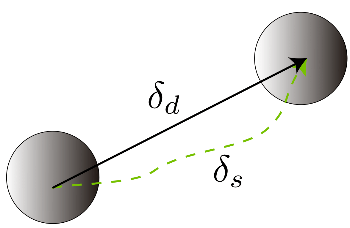
The discrete-time model is given as follows:
- [math]\displaystyle{ x_{{\langle k+1 \rangle}}= f(x_{{\langle k \rangle}}, \delta_{{\langle k \rangle}}, v_{ {\langle k \rangle}}) }[/math]
The new configuration in terms of the previous configuration and odometry, together with the error in the odometry as continuous random variables, can be defined as:
- [math]\displaystyle{ \xi_{{\langle k+1 \rangle}}= \begin{bmatrix} x_{{\langle k \rangle}}+ (\delta_{d,{{\langle k \rangle}}}+v_d)\cos(\theta_{{\langle k \rangle}}+\delta_\theta + v_\theta)\\ y_{{\langle k \rangle}}+ (\delta_{d,{{\langle k \rangle}}}+v_d)\sin(\theta_{{\langle k \rangle}}+\delta_\theta + v_\theta)\\ \theta_{{\langle k \rangle}}+ \delta_\theta + v_\theta \end{bmatrix} }[/math]
[math]\displaystyle{ \delta_d }[/math]: movement in x direction [math]\displaystyle{ \delta_\theta }[/math]: rotation [math]\displaystyle{ v_d, v_\theta }[/math]: error in odometry
Laser Range Finder
The laser range finder can provide observations with regards to the robot as described by
- [math]\displaystyle{ z = h(x_v, x_f, w), }[/math]
where [math]\displaystyle{ x_v }[/math] is the vehicle state, [math]\displaystyle{ x_f }[/math] is the location of the feature in the world frame and [math]\displaystyle{ w }[/math] is a random variable that models the sensor error.
The observation of the i-th feature [math]\displaystyle{ x_{f,i} }[/math] is expressed by
- [math]\displaystyle{ z = \begin{bmatrix} r\\\beta \end{bmatrix} = \begin{bmatrix} \sqrt{(y_i - y_v)^2 + (x_i - x_v)^2}\\ \tan{^{-1} }\frac{y_i-y_v}{x_i - x_v} - \theta_v \end{bmatrix} + \begin{bmatrix} w_r\\w_\beta \end{bmatrix}, }[/math]
with [math]\displaystyle{ r }[/math] is the range, [math]\displaystyle{ \beta }[/math] is the bearing angle and the measurement noise is given by
- [math]\displaystyle{ \begin{bmatrix} w_r\\ w_\beta \end{bmatrix} \sim N(0,W) }[/math]
- [math]\displaystyle{ W = \begin{bmatrix} \sigma_r^2 &0\\0&\sigma_\beta^2 \end{bmatrix}. }[/math]
Estimated uncertainty [math]\displaystyle{ \sigma_r = 0.1 }[/math] m and [math]\displaystyle{ \sigma_\beta = 1^\circ }[/math].
The observation by the LRF is linearized:
- [math]\displaystyle{ z_{{\langle k \rangle}}= \hat{h} + H_x(x_{{\langle k \rangle}}- \hat{x}_{{\langle k \rangle}}) + H_w w_{{\langle k \rangle}}, }[/math]
where the Jacobians are given by
- [math]\displaystyle{ H_{x_i} = \left. \frac{\partial h}{\partial x_v}\right|_{w=0} = \begin{bmatrix} -\frac{x_i - x_{v,{{\langle k \rangle}}}}{r} &-\frac{y_i - y_{v,{{\langle k \rangle}}}}{r} &0\\ \frac{x_i - x_{v,{{\langle k \rangle}}}}{r^2} &-\frac{y_i - y_{v,{{\langle k \rangle}}}}{r^2} &-1 \end{bmatrix} }[/math]
- [math]\displaystyle{ H_w = \left.\frac{\partial h}{\partial w}\right|_{w = 0} = \begin{bmatrix} 1 &0\\0&1 \end{bmatrix} }[/math]
Extended Kalman Filter
Given noisy odometry data, how can we estimate new pose given previous pose and noisy odometry? Kalman filter provides optimal estimate of the system state assuming zero mean Gaussian noise.
The used motion model is a non-linear model. Therefore the motion model is locally linearized wrt the current state estimate [math]\displaystyle{ \hat{x}_{{\langle k \rangle}} }[/math], resulting in
- [math]\displaystyle{ \hat{x}_{{\langle k+1 \rangle}}= \hat{x}_{{\langle k \rangle}}+ F_x(x_{{\langle k \rangle}}- \hat{x}_{{\langle k \rangle}}) + F_v v_{{\langle k \rangle}}, }[/math]
where [math]\displaystyle{ F_x = \frac{\partial f}{\partial x} }[/math] and [math]\displaystyle{ F_v = \frac{\partial f}{\partial v} }[/math] are Jacobians. These are obtained by differentiating and evaluating for [math]\displaystyle{ v = 0 }[/math]:
- [math]\displaystyle{ F_x = \left.\frac{\partial f}{\partial x}\right|_{v=0} = \begin{bmatrix} 1 & 0 &-\delta_{d,{{\langle k \rangle}}} - \sin(\theta_{{\langle k \rangle}}+ \delta_\theta)\\ 0&1&\delta_{d,{{\langle k \rangle}}}\cos(\theta_{{\langle k \rangle}}+ \delta_\theta)\\ 0&0&1 \end{bmatrix} }[/math]
- [math]\displaystyle{ F_v = \left.\frac{\partial f}{\partial v}\right|_{v=0} = \begin{bmatrix} \cos(\theta_{{\langle k \rangle}}+\delta_\theta) &-\delta_{d,{{\langle k \rangle}}}\sin(\theta_{{\langle k \rangle}}+ \delta_\theta)\\ \sin(\theta_{{\langle k \rangle}}+\delta_\theta)&\delta_{d,{{\langle k \rangle}}}\cos(\theta_{{\langle k \rangle}}+ \delta_\theta)\\ 0&1 \end{bmatrix} }[/math]
Preliminaries
- Define the initial state covariance [math]\displaystyle{ P_0 }[/math].
The values of the elements of this matrix can be small given that a good initial state estimation is assumed. - Define the estimate of the odometry covariance ([math]\displaystyle{ V }[/math]) [math]\displaystyle{ , \hat{V} }[/math].
Some experimentation is required to determine an appropriate value of [math]\displaystyle{ \hat{V} }[/math]. - Determine the estimated LRF covariance [math]\displaystyle{ \hat{W} }[/math]
Steps
The steps are as follows:
- EKF Prediction Equations
- [math]\displaystyle{ \hat{x}_{\langle k+1 | k\rangle} = f(\hat{x}_{\langle k\rangle}, \delta_{\langle k \rangle}, 0) }[/math]
- [math]\displaystyle{ \hat{P}_{{{\langle k+1 | k \rangle}}} = F_{x, \langle k \rangle}\hat{P}_{{\langle k | k \rangle}}F_{x, \langle k \rangle}{^\top}+ F_{v, \langle k \rangle }\hat{V} F_{v, \langle k \rangle}{^\top} }[/math]
- EKF Sensor Update Equations [math]\displaystyle{ \hat{x}_{{\langle k+1 | k+1 \rangle}}= \hat{x}_{{\langle k+1 | k \rangle}}+ K_{{\langle k+1 \rangle}}\nu_{{\langle k+1 \rangle}} }[/math][math]\displaystyle{ \hat{P}_{{\langle k+1 | k+1 \rangle}}= \hat{P}_{{\langle k+1 | k \rangle}}F_{x,{{\langle k \rangle}}}{^\top}- K_{{\langle k+1 \rangle}}H_{x,{{\langle k+1 \rangle}}}\hat{P}_{{\langle k+1 | k \rangle}} }[/math][math]\displaystyle{ S_{{\langle k+1 \rangle}}= H_{x,{{\langle k+1 \rangle}}} \hat{P}_{{\langle k+1 | k \rangle}}H_{x,{{\langle k+1 \rangle}}}{^\top}+ H_{w,{{\langle k+1 \rangle}}}\hat{W}_{{\langle k+1 \rangle}}H_{w,{{\langle k+1 \rangle}}}{^\top} }[/math][math]\displaystyle{ K_{{\langle k+1 \rangle}}= \hat{P}_{{\langle k+1 | k \rangle}}H_{x,{{\langle k+1 \rangle}}}{^\top}S_{{\langle k+1 \rangle}}{^{-1} } }[/math]
Sensor Fusion
The EKF framework allows data from many and varied sensors to update the state. This is the reason the estimation problem is also referred to as sensor fusion. Compass heading angle, GPS position, gyroscope yaw rate and target bearing angle can be all used to update the state.
All that is needed is
- Observation function [math]\displaystyle{ h(.) }[/math]
- Jacobians [math]\displaystyle{ H_x }[/math] and [math]\displaystyle{ H_w }[/math]
- Estimate of sensor output covariance [math]\displaystyle{ W }[/math]
The observation function [math]\displaystyle{ h(.) }[/math] can be both non-linear and non-invertible, the EKF does the rest.
Map Making
- [math]\displaystyle{ \hat{x}=(x_1, y_1,\dots, x_m, y_m){^\top} }[/math]
Now the prediction equations are as follows
- [math]\displaystyle{ \hat{x}_{{\langle k+1 | k \rangle}}= \hat{x}_{{\langle k | k \rangle}} }[/math]
- [math]\displaystyle{ \hat{P}_{{\langle k+1 | k \rangle}}= \hat{P}_{{\langle k | k \rangle}} }[/math]
With the state vector evolution
[math]\displaystyle{ g(x_v,z) = \begin{bmatrix} x_v + r_z\cos(\theta_v + \theta_z)\\ y_v + r_z\sin(\theta_v + \theta_z) \end{bmatrix} }[/math]
Adding landmarks can be done according to
- [math]\displaystyle{ x_{{\langle k | k \rangle}}^\star = y(x_{{\langle k | k \rangle}}, z_{{\langle k \rangle}}, x_{v,{{\langle k | k \rangle}}}) = \begin{bmatrix} x_{{\langle k | k \rangle}}\\ g(x_{v,{{\langle k | k \rangle}}}, z_{{\langle k \rangle}}) \end{bmatrix} }[/math]
The state vector with estimated coordinates to [math]\displaystyle{ m }[/math] landmarks can be described as
Simultaneous Localization and Mapping
The state vector consists of both the pose as the coordinates of the [math]\displaystyle{ M }[/math] landmarks that have been seen thus far:
- [math]\displaystyle{ \hat{x} = (x_v, y_v, \theta_v, x_1, y_1, ... , x_m, y_m) }[/math]
The covariance matrix is given by:
- [math]\displaystyle{ \hat{P} = \begin{bmatrix} \hat{P_{vv}} &\hat{P}_{vm}\\ \hat{P}_{vm}{^\top}&\hat{P_{mm}} \end{bmatrix} }[/math]
When a new feature is observed, the state vector is updated, where [math]\displaystyle{ G_x }[/math] is now non-zero and given by:
- [math]\displaystyle{ G_x = \frac{\partial g}{\partial x_v} = \begin{bmatrix} 1 &0 &-r_z\sin(\theta_v + \theta_z)\\ 0 &1 &r_z\cos(\theta_v + \theta_z) \end{bmatrix} }[/math]
as the estimate of the new feature depends on the state vector, which now contains the robot’s pose.
Feature observation changes wrt the state vector are described by the Jacobian [math]\displaystyle{ H_x }[/math]. The observation depends on:
- robot position
- position of observed feature
- [math]\displaystyle{ H_x = \left(H_{x_v} \dots 0 \dots H_{x_i} \dots 0\right), }[/math]
where [math]\displaystyle{ H_{x_i} }[/math] is at the location corresponding to [math]\displaystyle{ x_i }[/math]. [math]\displaystyle{ H_{x_v} }[/math] has been added at the beginning to account for the position of the robot.
Global and local path planning (Target, potential field and drive)
Maze solving
To solve the maze in an efficient way, Pico should know where to go based on information where it has been. A very efficient way of maze solving (when the maze is unknown and contains loops) is the Tremaux algorithm. The algorithm needs information from the map about which node it is approaching and in which direction it is approaching it. Based on this information it can determine which way to go. When a new node is reach it will take a random direction. When a node is already encountered before it will first take a direction it has not been yet. When every direction is already been taken at a junction it will turn around. Using this algorithm it will never get stuck in a loop and it should always find the exit, if there is no exit it will always return to its starting position.
For the maze challenge this algorithm was not implemented due to the fact that the mapping was not working good enough. When mapping does not work the above algorithm definitely won't work. For the maze challenge a random walk is implemented, which means that at every node it will make a random choice which direction it will continue. Because the maze is not really big (size of robocup field) it should be able to solve the maze using random walk.
Potential field
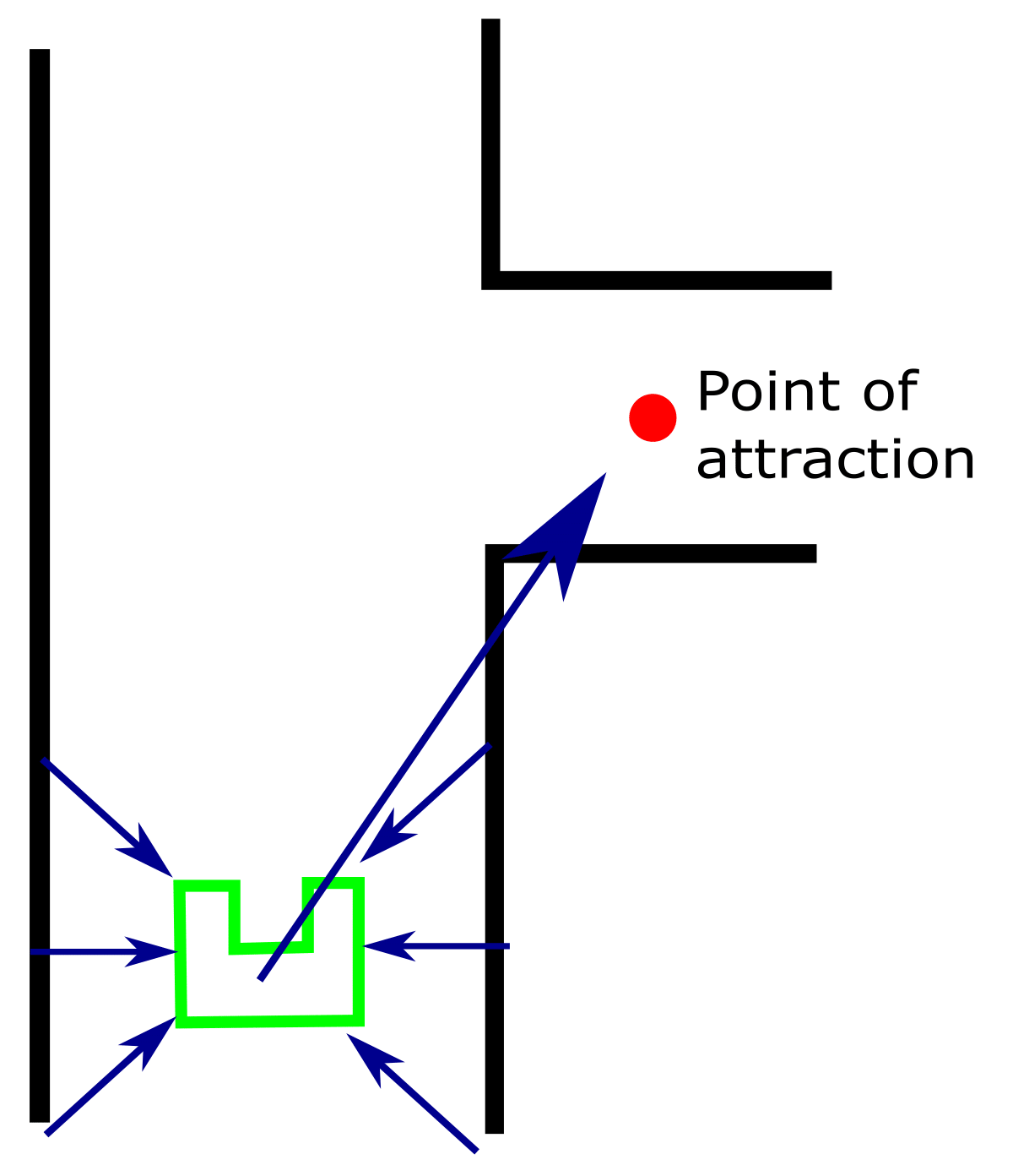
Pico is driving in the maze using a potential field, the potential field consists of virtual forces generated by the wall which are acting Pico. These forces are applied by every measurement point of the LRF data and are in the direction as the vector from the LRF point to Pico. The value of the force is based on the distance between Pico and the point, when the distance is becoming smaller the force should be bigger (to repel Pico from the wall), the value of the force is determined by the following equation
- [math]\displaystyle{ F_i = \frac{1}{r_i^5} }[/math]
with [math]\displaystyle{ F_i }[/math] the force acting on Pico due to the point [math]\displaystyle{ i }[/math] and [math]\displaystyle{ r_i }[/math] the distance between Pico and the point [math]\displaystyle{ i }[/math]. Using the summation of all these forces gives a force in the x and y direction which are used to determine a x, y and rotational velocity. To get a nice balance between these speed gain have been tuned for these speed during tests for different widths of corridors.
To take turns using the potential field a force of attraction is used as shown in Figure 12. This force is added to the repelling forces from the walls and thus pico will drive towards this point.
Furthermore the potential field is used as collision avoidance as well. Because when it is implemented in a good way it is impossible to drive into the wall when it is active.
The final maze challenge
The 9th of June was the date of the maze challenge. In the link below a video is shown of our attempt at the maze challenge. As shown Pico does drive out of the maze but it is not in a very nice way. At the beginning it drives towards the wall which is ahead of him, this happens because Pico does not recognize the nodes in the right way. Due to the potential field it does not drive into the wall and slowly rotates and keeps driving around in the maze. At about 55 seconds it stands in the doorway and after some time it recognizes it and opens the door. But because Pico is not orientated with his front to the door it does not see that in front of him the distance becomes larger and thus it recognizes it as a dead end and turns around. Then Pico starts driving on its potential field again and finally at around 1:50 it reaches the openspace again and on just its potential field with a force in the x direction it reaches the exit in a little over 2 minutes.
The YouTube video of the solved maze challenge can be found here: The maze challenge solved
Based on this result it is concluded that the node recognition is not working good enough, therefore some adjustments are made and implemented in the simulator. A simulation on the same maze is conducted. As shown in the video in the link below the maze is successfully solved in simulations as well.
The YouTube video of the solved maze in the simulator can be found here: The maze challenge solved in the simulator
Conclusions and recommendations
Conclusions
First of all it can be concluded that both goals are achieved, the corridor and the maze challenge are solved.
Furthermore some conclusions are drawn about the progress of the project. During the project we encountered some problems, the first problem was the lack of experience in C++. No one in the group had experience in programming C++, this required some time in the beginning of the project. Then during the corridor challenge the result was good, but the problem with the code that was used, that most of it was not reusable for the maze challenge. Since for the maze challenge it is not just take a turn right or left, which was the only thing that in the corridor challenge which was detected. The part that is used for the maze challenge is the potential field, which worked very well.
Then for the maze challenge some new problems occurred. The most important problem occurred due to the fact that the code became much bigger. It was hard to keep the code structured and to merge different parts of code, because multiple people where working on the code sometimes it became hard to understand every part of it.
Another important lesson learned is to write the code in such a way that it is easy scalable and reusable for similar problems, this is done by making the "magic number" clear and understandable.
Another problem occurred while testing, because the LRF showed some points in the real setup which were not there and thus had to be filtered out. Furthermore it must be able to work with gaps between walls. Also the tuning of the potential field had to be done for both the simulator as the real setup, because values that worked in the simulator did not make Pico drive smooth in reality.
Furthermore it would have been helpful if we had one more group member, because the study load was more then 5 ECTS.
Recommendations
For future projects some recommendations are done. The first recommendation is that in the future a more structured approach should be used. Because the code becomes quite large it is important to make a clear overview of what function does what. Furthermore it is important to make more clear agreements within the group about what every function does (what does it get from other functions and what should it produce). Also it is important to start more easy. For example the SLAM algorithm which was immediately written with extended kalman filter etc. Maybe a more straightforward approach would have been better to start with.
Documents
- Initial design document (week 1): File:InitialDesignIdea - Group 4.pdf
- Design presentation (week 4): File:Design Presentation.pdf
- Final presentation (week 8): File:Final Presentation.pdf