Embedded Motion Control 2012 Group 5: Difference between revisions
| (10 intermediate revisions by 4 users not shown) | |||
| Line 47: | Line 47: | ||
** Finish the LRF-vision | ** Finish the LRF-vision | ||
** Start with the strategy for the corridor competition | ** Start with the strategy for the corridor competition | ||
* ''' | * '''Week 5 (May 21<sup>th</sup> - May 27<sup>th</sup>)'' | ||
* ''' | ** Edit the action handler with PD control | ||
* ''' | ** Creating a version of the action handler, simple_follower, for the corridor competition | ||
* ''' | ** Testing on the robot | ||
* ''' | |||
* '''Week 6 (May 28<sup>th</sup> - June 3<sup>rd</sup>)''' | |||
**Start Canny based arrow recognition | |||
**Working on LRF vision | |||
* '''Week 7 (June 4<sup>th</sup> - June 10<sup>rd</sup>)''' | |||
**Finished LRF vision, working on the mapping node | |||
**Starting CG based arrow recognition | |||
* '''Week 8 (June 11<sup>th</sup> - June 17<sup>rd</sup>)''' | |||
**Working on the mapping node | |||
**Testing on the robot | |||
**Working on arrow recognition | |||
* '''Week 9 (June 18<sup>th</sup> - June 24<sup>rd</sup>)'' | |||
** Final contest preparation | |||
** Testing on the robot | |||
** Working on the mapping node | |||
===Agreements=== | ===Agreements=== | ||
| Line 130: | Line 145: | ||
'''end''' | '''end''' | ||
'''if''' false_points_counter > | '''if''' false_points_counter > MAX_FALSE_POINTS | ||
'''then''' end the line | '''then''' end the line | ||
decrease the data point index with | decrease the data point index with MAX_FALSE_POINTS | ||
create a new line with the first two points | create a new line with the first two points | ||
increase the line index with 1 | increase the line index with 1 | ||
| Line 139: | Line 154: | ||
'''LRF processed data''' | '''LRF processed data / Map creation and navigation''' | ||
The output of the line detection algorithm is published on /lines, and the ''map''-node is subscribed to this topic. This node corrects for the robot's movement during each time-step and then matches the newly detected lines to the lines it has stored earlier (or adds new lines to the | The output of the line detection algorithm is published on /lines, and the ''map''-node is subscribed to this topic. This node corrects for the robot's movement during each time-step and then matches the newly detected lines to the lines it has stored earlier (or adds new lines to the buffer if no matches are found, when 3 lines in the buffer are the same, they are added to the map). A simple corner detection algorithm is ran once every second and used to fixate lines; if the endpoints of two lines match, these are considered a corner and will be 'locked', preventing them from being moved and allowing the robot to establish its position in relation to these points. These corners are also used to determine the junctions in the maze, after which the possible directions for each junction are determined. This combination of junctions and possible directions become the 'nodes' which the robot uses to decide where to go. | ||
The figure below shows four stages of the robot's automated exploration. From left to right: | The figure below shows four stages of the robot's automated exploration. From left to right: | ||
| Line 148: | Line 163: | ||
# As only part of the maze is visible, the robot does not yet recognize the dead end properly. | # As only part of the maze is visible, the robot does not yet recognize the dead end properly. | ||
# After continuing a bit, the third wall of the dead end becomes visible and the node is updated accordingly. | # After continuing a bit, the third wall of the dead end becomes visible and the node is updated accordingly. | ||
When no intersection is found, the robot will explore the maze in a direction that is still possible according to the current node (see video below). When entering a dead end behind a corner, the robot follows back its path and continues in a direction that is not yet explored. | |||
Because the absolute position of the robot in the maze is known, it calculates a setPoint to which it can directly drive (i.e. it does not run into walls). The speed depends on the angle to the setPoint (the larger the angle, the smaller the forward speed, and the larger the angular speed). The ''map''-node saves the route and checks whether or not there is a shorter route to the current location. When this is the case, the route is replaced by the shorter one. | |||
[[File:MazePlotting.jpg|1200px]] | [[File:MazePlotting.jpg|1200px]] | ||
| Line 172: | Line 190: | ||
cvCvtColor(rgbImg, hsvImg, CV_BGR2HSV); | cvCvtColor(rgbImg, hsvImg, CV_BGR2HSV); | ||
Since HSV data is available now, we can determine for each pixel it is red or not. This segmentation leads to a binary image that is displayed in color segmented image which is shown above. To reduce noise in the image and to sharpen the corners of the arrow, an erosion filter ('''cvErode()''') is applied twice with a 3x3 pixels structuring element. Moreover, a canny algorithm ('''cvCanny()''') is used to detect the bounding lines of the arrow. The result of this filtering is shown in the third figure: 'Line detection' . | Since HSV data is available now, we can determine for each pixel if it is red or not. This segmentation leads to a binary image that is displayed in color segmented image which is shown above. To reduce noise in the image and to sharpen the corners of the arrow, an erosion filter ('''cvErode()''') is applied twice with a 3x3 pixels structuring element. Moreover, a canny algorithm ('''cvCanny()''') is used to detect the bounding lines of the arrow. The result of this filtering is shown in the third figure: 'Line detection' . | ||
The next step in the arrow detection process is to detect the seven corners that determine the shape of the arrow. This is done by calling another openCV function: '''cvGoodFeaturesToTrack()''' | The next step in the arrow detection process is to detect the seven corners that determine the shape of the arrow. This is done by calling another openCV function: '''cvGoodFeaturesToTrack()''' | ||
| Line 191: | Line 209: | ||
With these corners available, the last step in the arrow detection algorithm can be executed. By looping over the corners, the highest and lowest corner can be found, with these two points, the perpendicular bisector of these points can be constructed. The blue line in the last picture represents this line. In the most ideal case, the tip of the arrow would be exactly located at this line. Therefore, the corners that located at minimal distance from this bisector, is expected to be the tip of the arrow. If this corners is located left with respect to the average of the points that construct the bisector, the arrow points to left. In the contrary case, the arrow points right. | With these corners available, the last step in the arrow detection algorithm can be executed. By looping over the corners, the highest and lowest corner can be found, with these two points, the perpendicular bisector of these points can be constructed. The blue line in the last picture represents this line. In the most ideal case, the tip of the arrow would be exactly located at this line. Therefore, the corners that located at minimal distance from this bisector, is expected to be the tip of the arrow. If this corners is located left with respect to the average of the points that construct the bisector, the arrow points to left. In the contrary case, the arrow points right. | ||
The algorithm | ====Simple algorithm==== | ||
The algorithm described in the previous section works fine, as long as the provided images are of good quality and high resolution. However, due to the fish-eye effect and the low resolution of Jazz's webcam, the quality of the images is not sufficient. Therefore, after filtering the images, the sharpness of the remaining blob is not sufficient to distinguish the characteristic corners of the arrow. Therefore, a less demanding algorithm is implemented, based on the algorithm described by groups 3 and 9. However, the filtering before this algorithm is applied is extended. | |||
First the binary image is duplicated, after which an erosion is applied, followed by two dilation steps. This results in an image where all the small blobs are removed, and large blobs are bigger than in the original image. This filtered image is compared with the original image and only the pixels that have high value in both images are maintained. | |||
The next step is clustering red objects in the image, using a [http://en.wikipedia.org/wiki/K-means_clustering k-means algorithm]. The result of this algorithm is analyzed to check if the largest clusters are located very close to each other. In that case, the arrow is probably spread over multiple clusters. Therefore, large clusters that are close to each other are combined. If the largest (combined) cluster contains at least 300 pixels, it is assumed to be the arrow. | |||
This k-means filtering leads to a binary image that contains only the arrow and therefore is suitable for applying the algorithm described by groups 3 and 9. | |||
== Strategies == | == Strategies == | ||
| Line 222: | Line 242: | ||
# The robot continues through the maze until it eventually reaches the exit… | # The robot continues through the maze until it eventually reaches the exit… | ||
[[File:NodeBasedMazeSolvingUnknown.jpg]] | [[File:NodeBasedMazeSolvingUnknown.jpg]] | ||
====Node-based Mapping 2==== | |||
A simpler alternative to the method described above consists of implementing a Trumeaux-style algorithm which does not require the ability to look 'ahead' in the maze to detect dead ends prematurely (although this would improve its efficiency). | |||
This is done by giving storing not only the locations of each node and the directions the robot can travel in, but also the node which it will reach by traveling in a certain direction (with 0 representing an unknown direction and NaN, Inf, or another similar non-integer representing directions which point to a wall). Whenever the robot reaches a node, it will take the direction leading to the lowest number; this will be one into the unknown if one is available, or the direction leading back to the point from which this one was reached if not. This is demonstrated by the figures below, in which all consciously chosen routes are given by the blue numbers: | |||
# The robot has reached a point from which two directions lead into the unknown and chooses one of them (possibly randomly). | |||
# Another choice is available and the robot picks the direction leading into the unknown (as opposed to the one leading back to node 4. | |||
# As this node marks the end of a path, the robot can only to the last node it visited. | |||
# The robot retraces its steps by choosing the lowest value at each point, causing it to end up in the other branch of the junction. | |||
# From this point, the robot will explore the second path. | |||
# Once again, the robot encounters a dead end and is forced to turn around. | |||
# The robot retraces its steps a second time, but this time the lowest value at the central node is that of node 3 through which it entered this section of the maze. Therefore, the robot leaves through the bottom path. | |||
[[File:NodeBasedPlanB.jpg]] | |||
====Grid based maze solving==== | ====Grid based maze solving==== | ||
| Line 227: | Line 263: | ||
[[File:GridBasedMazeSolving.png]] | [[File:GridBasedMazeSolving.png]] | ||
====Final Contest and improvements made==== | |||
[Video of the map in action after improvements [https://www.dropbox.com/s/jpt4fhb9mnglieg/out-9.ogv]] | |||
The shivering lines (white and light blue) are the line jazz currently sees and uses to position itself in the map. | |||
The orange cross is the next setPoint, the white line in the middle of the paths is the shortest route to the current position. | |||
Some improvements to the existing code: the robot now orientates itself perpendicular to the map before it starts driving, so navigation is easier and more accurate. Furthermore the robot now starts exploring in forward direction, even if it has not found any intersections yet (this to prevent it from staying at its starting position). | |||
The visualisation of the map is improved as well, it now shows the setPoint of the robot and shows the shortest path to the exit of the maze. | |||
Latest revision as of 23:11, 1 July 2012
Group Information
| Name | Student number | Build |
|---|---|---|
| Fabien Bruning | 0655273 | Ubuntu 10.10 on Virtualbox in OSX 10.7 |
| Yanick Douven | 0650623 | Ubuntu 10.04 dual boot with W7 |
| Joost Groenen | 0656319 | Ubuntu 10.04 dual boot with W7 |
| Luuk Mouton | 0653102 | Ubuntu 10.04 dual boot with W7 (Wubi) |
| Ramon Wijnands | 0660711 | Installed Ubuntu with wubi (included with the Ubuntu CD) |
Planning and agreements
Planning by week
- Week 1 (April 23th -April 29)
- Install Ubuntu and get familiar with the operating system
- Week 2 (April 30th - May 6th)
- Get the software environment up and running on the notebooks
- ROS
- Eclipse
- Gazebo
- Start with the tutorials about C++ and ROS
- Get the software environment up and running on the notebooks
- Week 3 (May 7th - May 13th)
- Finish the tutorials about C++ and ROS
- Install smartsvn
- Create a ROS package and submit it to the SVN
- Read chapters of the book up to chapter 7
- Make an overview of which elements of chapter 7 should be covered during the lecture
- Week 4 (May 15th - May 20th)
- Make lecture slides and prepare the lecture
- Finish the action handler
- Finish the LRF-vision
- Start with the strategy for the corridor competition
- 'Week 5 (May 21th - May 27th)
- Edit the action handler with PD control
- Creating a version of the action handler, simple_follower, for the corridor competition
- Testing on the robot
- Week 6 (May 28th - June 3rd)
- Start Canny based arrow recognition
- Working on LRF vision
- Week 7 (June 4th - June 10rd)
- Finished LRF vision, working on the mapping node
- Starting CG based arrow recognition
- Week 8 (June 11th - June 17rd)
- Working on the mapping node
- Testing on the robot
- Working on arrow recognition
- 'Week 9 (June 18th - June 24rd)
- Final contest preparation
- Testing on the robot
- Working on the mapping node
Agreements
- For checking out the svn and committing code, we will use Smartsvn
- Add your name to the comment when you check in
- Every Tuesday, we will work together on the project
- Every Monday, we will arrange a tutor meeting
Strategy and software description
Strategy
'Visual Status Report Because a picture is worth a thousand words.
ROS layout
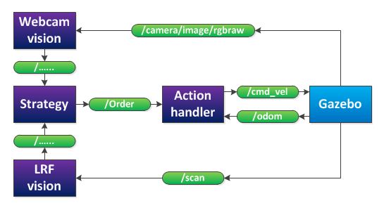
After a group discussing, we decided that our provisionally software layout will be as in the figure below.
The 'webcam vision' node processes the images, produced by the RGB-camera. It will publish if it detects an arrow and in what direction the arrow points. The 'LRF vision' node processes the data of the laser range finder. It will detect corners, crossroads and the distance to local obstacles. This will also be published to strategy. The 'strategy' node will decide, based on the webcam and LRF vision, what action should be executed (stop, drive forward, drive backward, turn left or turn right) and will publish this decision to the 'action handler' node. Finally, the 'action handler' node will send a message to the jazz-robot, based on the received task and on odometry data.
Movement Control
Action Handler
To ensure that the strategy node does not need to continuously 'spam' instructions to the actual robot, an intermediate node is installed to perform low-level actions. This node receives orders such as: "Go 1m forwards." (written as an order-amount pair) and translates them to a stream of instructions to the robot itself (over the /cmd_vel channel) which persists until the robot has travelled the desired amount. The two main difficulties with this method are the inaccuracy of the odometer data when moving and its limited range (between -1 and 1, fixed around the reference frame it pretends to know). To reduce the impact of these issues, the movement of the robot is measured relative to the point where it received the order instead of to its initial position. This procedure works as follows:
- As soon as the order is received, the node stores the current position and heading, and the first movement order is sent out.
- Every time the odometer data is updated, a callback is activated which determines the progress as shown in the figure below.
- For rotation, the change in angle is determined by finding the smallest distance between the current and previous angle. This change is added to the total change.
- For lateral movement, the absolute distance between the current and initial point is measured.
- If the change in angle or lateral movement exceeds the original target value, the node goes back to its default state and the robot stops moving.
Also, LRF data can be mixed with odometer data via a ROS package (laser_scanner_matching) to improve accuracy. Since a well documented ROS package called the "Laser Scan Matcher" is available, we opted to use this instead of developing our own algorithm. The package is largely based on the work by Andrea Censi, described in his paper 'An ICP variant using a point-to-line metric" (2008). It basically works as follows:
- At time [math]\displaystyle{ k }[/math], the laser scanner measures a set of points [math]\displaystyle{ p }[/math].
- At time [math]\displaystyle{ k+1 }[/math], the laser scanner measures a set of points [math]\displaystyle{ p_{k+1} }[/math]. This set of points is presumed to be the same set of points translated and rotated by an operator [math]\displaystyle{ q }[/math].
- A minimization of the error between [math]\displaystyle{ p_{k} }[/math], operated on by operator [math]\displaystyle{ q }[/math], and [math]\displaystyle{ p_{k+1} }[/math] is now performed, which yields [math]\displaystyle{ q }[/math].
Of course, the new set of points does not exactly match the original set of points exactly and the data is noisy. The paper deals with a multitude of tricks to optimize the algorithm.
PD-Control
As the real robot is even less accurate than the one in the simulator, simply ordering it to move directly forwards will most likely result in a collision with the walls before the next corner is reached. To remedy this, forwards movement is controlled by a simple PD-controller which compares the distance to the walls on either side of the robot and steers away from the nearest one. The 'D'-action is required to smooth the movement and prevent unnecessary 'wriggling' when moving through a long corridor.
Mapping
LRF vision
The Laser Range Finder of the Jazz robot is simulated in the jazz_simulater with 180 angle increments from -130 to 130 degrees. The range is 0.08 to 10.0 meters, with a resolution of 1 cm and an update rate of 20 Hz. The topic is /scan and is of the type sensor_msgs::LaserScan. The data is clipped at 9.8 meters, and the first and last 7 points are discarded, since these data points lie on the jazz robot.
The LRF data can be processed in multiple ways. Since it not exactly clear what the GMapping algorithm (implemented in ROS) does, we decided to write our own mapping algorithm. But first the LRF needs to be interpreted. Therefore, a class is created that receives LRF data and fits lines through the data. The fitting of lines can be done in two ways; a hough transform and a fanciful algorithm.
Hough transform
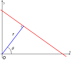
A hough transform interprets the data points of the LRF in a different way; each point in x-y-space can be seen as a point through which a line can be drawn. This line will be of the form [math]\displaystyle{ y=ax+b }[/math], but can also be parametrized in polar coordinates. The parameter [math]\displaystyle{ r }[/math] represents the distance between the line and the origin, while [math]\displaystyle{ \theta }[/math] is the angle of the vector from the origin to this closest point. Using this parameterization, the equation of the line can be written as
- [math]\displaystyle{ y = \left(-{\cos\theta\over\sin\theta}\right)x + \left({r\over{\sin\theta}}\right) }[/math]
So for an arbitrary point on the image plane with coordinates ([math]\displaystyle{ x_0 }[/math], [math]\displaystyle{ y_0 }[/math]), the lines that go through it are the pairs ([math]\displaystyle{ r }[/math],[math]\displaystyle{ \theta }[/math]) with
- [math]\displaystyle{ r(\theta) =x_0\cdot\cos \theta+y_0\cdot\sin \theta }[/math]
Now a grid can be created for [math]\displaystyle{ \theta }[/math] and [math]\displaystyle{ r }[/math], in which all pairs ([math]\displaystyle{ r }[/math],[math]\displaystyle{ \theta }[/math]) are drawn. Now a 3D surface is created that shows peaks for the combinations of [math]\displaystyle{ \theta }[/math] and [math]\displaystyle{ r }[/math] that are good fits for lines in the LRF data.
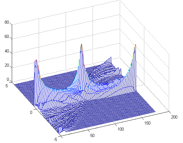
In the figure on the right this transform has been performed on the LRF data. Several peaks can be seen that represent walls. The difficulty with this transform is the selection of the right peaks. This can be solved by using some image processing and some general knowledge on the LRF data. This method will however not be used by our group but it is kept in mind in case the fanciful algorithm fails.
Another drawback of this method is that holes in the wall are difficult to detect, since the line is parametrized with [math]\displaystyle{ \theta }[/math] and [math]\displaystyle{ r }[/math] and has therefore no beginning or end. This problem can be fixed by mapping all data points to the closest line and snipping the line in smaller pieces. An advantage is that a Hough transform is very robust, and can handle noisy data.
Fanciful algorithm
We thought of an own algorithm for line detection as well. Since the data is presented to the /scan topic in array of points with increasing angle, the points can be checked individually if they contribute to a line. A pseudocode version of the algorithm looks as follows:
create a line between point 1 and point 2 of the LRF data (LINE class)
loop over all data points
   l = current line
   p = current point
   if perpendicular distance between l and p < [math]\displaystyle{ \sigma }[/math] AND angle between l and p < 33 degrees AND dist(endpoint of l, a) < 40 cm
     // point is good and can be added to the line
     then add point to line
     else false_points_counter++
  end

  if false_points_counter > MAX_FALSE_POINTS
    then end the line
         decrease the data point index with MAX_FALSE_POINTS
         create a new line with the first two points
         increase the line index with 1
  end
end loop
LRF processed data / Map creation and navigation
The output of the line detection algorithm is published on /lines, and the map-node is subscribed to this topic. This node corrects for the robot's movement during each time-step and then matches the newly detected lines to the lines it has stored earlier (or adds new lines to the buffer if no matches are found, when 3 lines in the buffer are the same, they are added to the map). A simple corner detection algorithm is ran once every second and used to fixate lines; if the endpoints of two lines match, these are considered a corner and will be 'locked', preventing them from being moved and allowing the robot to establish its position in relation to these points. These corners are also used to determine the junctions in the maze, after which the possible directions for each junction are determined. This combination of junctions and possible directions become the 'nodes' which the robot uses to decide where to go.
The figure below shows four stages of the robot's automated exploration. From left to right:
- The robot begins and places the first point beneath itself and notices one corner in front of it.
- The robot has moved two junctions onwards and is now in the progress of ignoring the dead end and moving further up.
- As only part of the maze is visible, the robot does not yet recognize the dead end properly.
- After continuing a bit, the third wall of the dead end becomes visible and the node is updated accordingly.
When no intersection is found, the robot will explore the maze in a direction that is still possible according to the current node (see video below). When entering a dead end behind a corner, the robot follows back its path and continues in a direction that is not yet explored.
Because the absolute position of the robot in the maze is known, it calculates a setPoint to which it can directly drive (i.e. it does not run into walls). The speed depends on the angle to the setPoint (the larger the angle, the smaller the forward speed, and the larger the angular speed). The map-node saves the route and checks whether or not there is a shorter route to the current location. When this is the case, the route is replaced by the shorter one.

Vision
Webcam vision
 |
 |
 |
 |
 |
The images that are captured by Jazz's webcam, can be used to detect the arrows that will point him in the right direction. This section will describe the progress of the development of the Webcam vision node.
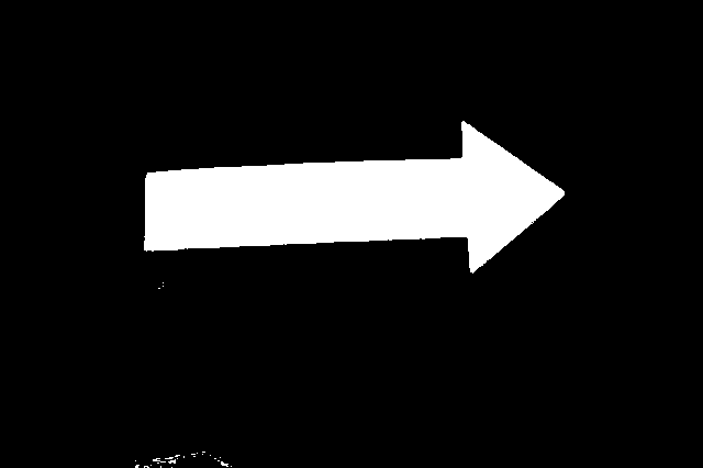
In the RGB colorspace, there are three channels (red, green and blue) that determine the color of a pixel. To detect red pixels, this does not give very large problems since it has it's own color channel in the RGB colorspace. However, it is easier to use the HSV colorspace (hue, saturation and value), where the color is only described by the hue, where the saturation and value determine how bright a pixel is. This makes it easier to describe which section of the colorspace is accepted as red. Therefore, the first step in the image processing is to convert the RGB image to the HSV colorspace. Using the openCV library makes this an easy task, using the cvCvtColor() function. For testing purposes, we used a webcam image that is loaded with cvLoadImage() (An example is given above in the first picture). This creates an image object in which the order of the channels is BGR instead of RGB. Therefore, the conversion is BGR to HSV instead of RGB to HSV.
IplImage *rgbImg, *hsvImg;

rgbImg = cvLoadImage("arrow2.jpg",CV_LOAD_IMAGE_COLOR);
hsvImg = cvCreateImage(cvGetSize(rgbImg), IPL_DEPTH_8U, 3 );

cvCvtColor(rgbImg, hsvImg, CV_BGR2HSV);
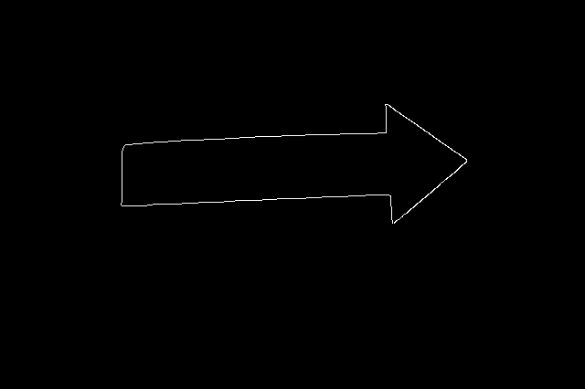
Since HSV data is available now, we can determine for each pixel if it is red or not. This segmentation leads to a binary image that is displayed in color segmented image which is shown above. To reduce noise in the image and to sharpen the corners of the arrow, an erosion filter (cvErode()) is applied twice with a 3x3 pixels structuring element. Moreover, a canny algorithm (cvCanny()) is used to detect the bounding lines of the arrow. The result of this filtering is shown in the third figure: 'Line detection' .
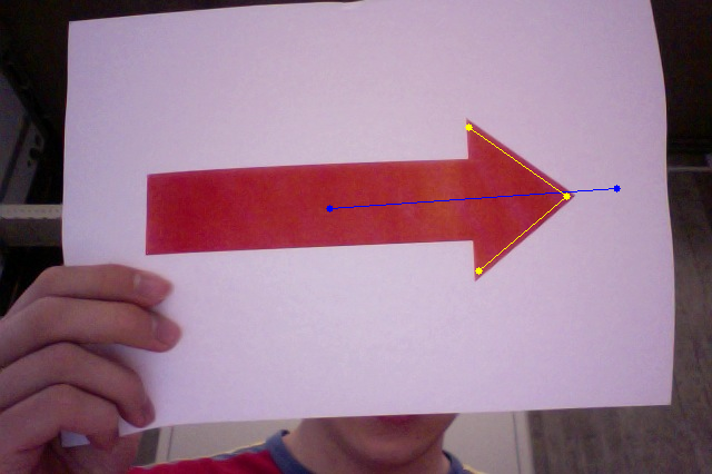
The next step in the arrow detection process is to detect the seven corners that determine the shape of the arrow. This is done by calling another openCV function: cvGoodFeaturesToTrack()
// Create temporary images required by cvGoodFeaturesToTrack
IplImage* imgTemp = cvCreateImage(cvGetSize(rgbImg), 32, 1);
IplImage* imgEigen = cvCreateImage(cvGetSize(rgbImg), 32, 1);

// Create array to store corners
int count = 15;
CvPoint2D32f* corners = new CvPoint2D32f[count];

// Find corners
cvGoodFeaturesToTrack(binImg, imgEigen, imgTemp, corners, &count, 0.1, 20);
This functions detects up to 15 corners in the image, depending on how accurate the image is. In the most optimal situation, only seven corners will be returned. Applying this algorithm leads to the fourth image shown above, where the detected corners are superimposed on the RGB-image.
With these corners available, the last step in the arrow detection algorithm can be executed. By looping over the corners, the highest and lowest corner can be found, with these two points, the perpendicular bisector of these points can be constructed. The blue line in the last picture represents this line. In the most ideal case, the tip of the arrow would be exactly located at this line. Therefore, the corners that located at minimal distance from this bisector, is expected to be the tip of the arrow. If this corners is located left with respect to the average of the points that construct the bisector, the arrow points to left. In the contrary case, the arrow points right.
Simple algorithm
The algorithm described in the previous section works fine, as long as the provided images are of good quality and high resolution. However, due to the fish-eye effect and the low resolution of Jazz's webcam, the quality of the images is not sufficient. Therefore, after filtering the images, the sharpness of the remaining blob is not sufficient to distinguish the characteristic corners of the arrow. Therefore, a less demanding algorithm is implemented, based on the algorithm described by groups 3 and 9. However, the filtering before this algorithm is applied is extended.
First the binary image is duplicated, after which an erosion is applied, followed by two dilation steps. This results in an image where all the small blobs are removed, and large blobs are bigger than in the original image. This filtered image is compared with the original image and only the pixels that have high value in both images are maintained.
The next step is clustering red objects in the image, using a k-means algorithm. The result of this algorithm is analyzed to check if the largest clusters are located very close to each other. In that case, the arrow is probably spread over multiple clusters. Therefore, large clusters that are close to each other are combined. If the largest (combined) cluster contains at least 300 pixels, it is assumed to be the arrow.
This k-means filtering leads to a binary image that contains only the arrow and therefore is suitable for applying the algorithm described by groups 3 and 9.
Strategies
Node-based Mapping
Storing the entire maze as a series of points (or even lines) consumes a lot of space; therefore it makes sense to store the known map of the world in a smaller format. One way to do this is by storing all of the junctions, corners, and endpoints as a set of nodes that keep track of the directions in which the robot can travel when it stands on one of them. Including the approximate distance to the next node for each direction is not required, but may help to prevent duplicate points after looping around or otherwise ending up at the same spot twice. Arrows or other ‘clues’ can easily be included by removing or adding paths as instructed.
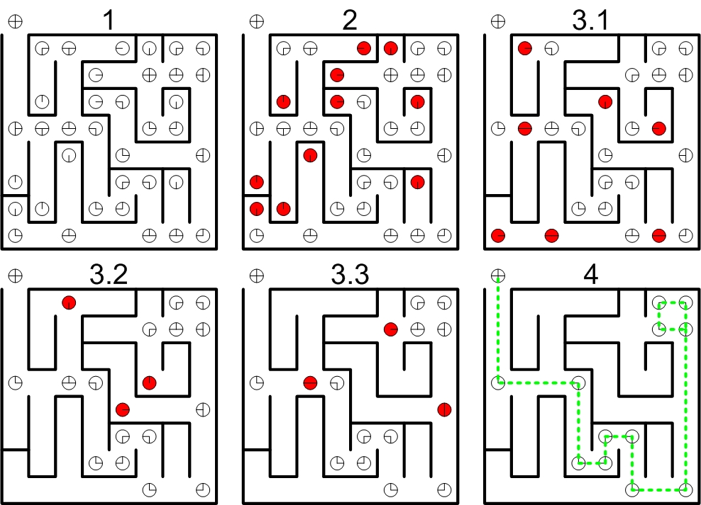
Node-based Known Maze Solving When the maze is known in nodular form, solving it becomes a trivial matter. The following procedure is demonstrated in the figure below.
- The maze is stored as a set of corner points, each with one to four directions of possible travel. The robot starts in the upper-right corner and needs to reach the exit in the upper-left.
- All nodes from which the robot can travel in only one direction are obviously dead ends.
- The dead ends are removed (with the possible exception of the robot’s starting position), after which the remaining nodes are updated. Because of this, further nodes will now become dead ends or straight paths. These are removed in turn and the process repeats until no more nodes are removed.
- The only remaining nodes are now the ones that lead from the robot’s initial position to the end of the maze.
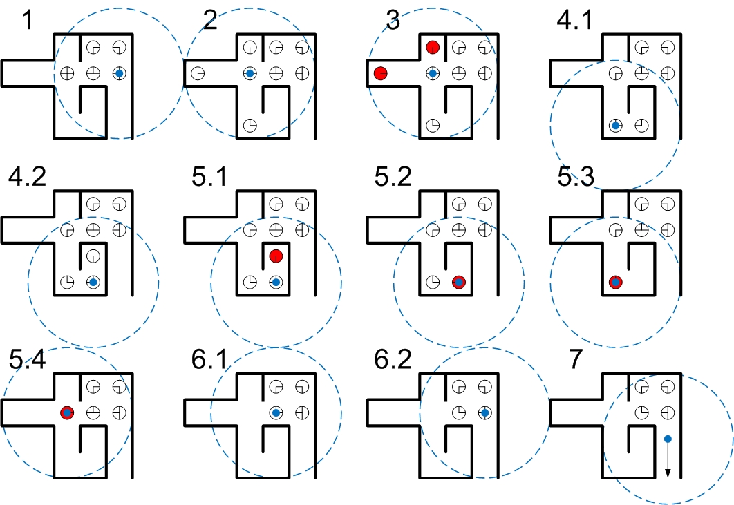
Node-based Unknown Maze Solving More interesting for the project is the scenario in which the maze is not yet known. This too can be solved using a node-based approach, as demonstrated here. In the image below, the blue dot represents the robot, and the surrounding circle the limit of its sensors.
- The robot begins and creates nodes for the area it can detect.
- It moves to the node which currently contains the most paths leading into the unknown (whilst avoiding immediate backtracking in case of ties) and updates its map.
- Dead ends are detected and removed as in the scenario with a known maze.
- The robot progresses deeper down its chosen path.
- Eventually, a dead end is reached which is eliminated. This in turn causes the node the robot is currently on to become a dead end. The robot moves back through the only possible path and then removes this new dead end. This procedure repeats as required.
- Upon returning to a node that does not have to be removed, the robot once again determines the node with the most paths leading into the unknown and moves to that node.
- The robot continues through the maze until it eventually reaches the exit…
Node-based Mapping 2
A simpler alternative to the method described above consists of implementing a Trumeaux-style algorithm which does not require the ability to look 'ahead' in the maze to detect dead ends prematurely (although this would improve its efficiency).
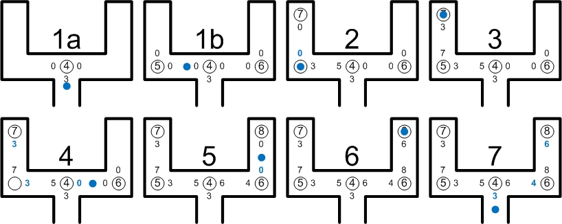
This is done by giving storing not only the locations of each node and the directions the robot can travel in, but also the node which it will reach by traveling in a certain direction (with 0 representing an unknown direction and NaN, Inf, or another similar non-integer representing directions which point to a wall). Whenever the robot reaches a node, it will take the direction leading to the lowest number; this will be one into the unknown if one is available, or the direction leading back to the point from which this one was reached if not. This is demonstrated by the figures below, in which all consciously chosen routes are given by the blue numbers:
- The robot has reached a point from which two directions lead into the unknown and chooses one of them (possibly randomly).
- Another choice is available and the robot picks the direction leading into the unknown (as opposed to the one leading back to node 4.
- As this node marks the end of a path, the robot can only to the last node it visited.
- The robot retraces its steps by choosing the lowest value at each point, causing it to end up in the other branch of the junction.
- From this point, the robot will explore the second path.
- Once again, the robot encounters a dead end and is forced to turn around.
- The robot retraces its steps a second time, but this time the lowest value at the central node is that of node 3 through which it entered this section of the maze. Therefore, the robot leaves through the bottom path.
Grid based maze solving
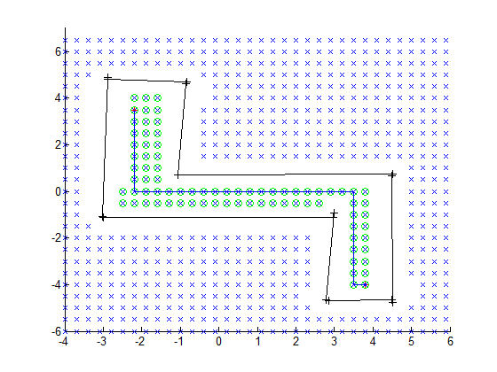
The odometry data is already converted into line segments so the next step is to move through the maze. A simple algorithm has been developed to drive trough the maze. First a grid is placed on the ground. Then all grid points that are closer than R meters from a line are removed. This ensures that all grid points can be visited by the robot, who has a smaller radius than R. In the figure below this grid can be seen. When a driving target is selected, with a simple breath-first search, all grid points are explored and the shortest route is calculated. The green dots are the points where the search is able to drive to. The blue line is the final path.
Final Contest and improvements made
[Video of the map in action after improvements [1]] The shivering lines (white and light blue) are the line jazz currently sees and uses to position itself in the map. The orange cross is the next setPoint, the white line in the middle of the paths is the shortest route to the current position.
Some improvements to the existing code: the robot now orientates itself perpendicular to the map before it starts driving, so navigation is easier and more accurate. Furthermore the robot now starts exploring in forward direction, even if it has not found any intersections yet (this to prevent it from staying at its starting position). The visualisation of the map is improved as well, it now shows the setPoint of the robot and shows the shortest path to the exit of the maze.
