Embedded Motion Control 2016 Group 3: Difference between revisions
| (99 intermediate revisions by 4 users not shown) | |||
| Line 114: | Line 114: | ||
|} | |} | ||
==Components== | === Components === | ||
PICO | The PICO robot consists of multiple components which are listed below: | ||
# Sensors: | # Sensors: | ||
## Laser Range Finder (LRF): | ## Laser Range Finder (LRF): Through the LRF on the PICO one can detect the distance to an object.This is accomplished by sending a laser pulse in a narrow beam towards the object and measuring the time taken by the pulse to be reflected on the target and returned to the sender. | ||
## Wheel encoders (odometry): The encoders will provide us with the speed of the wheels which can be used to control PICO based on the provided data. | ## Wheel encoders (odometry): The encoders will provide us with the speed of the wheels which can be used to control PICO based on the provided data. | ||
# Actuators: | # Actuators: | ||
| Line 169: | Line 169: | ||
===Collision avoidance=== | ===Collision avoidance=== | ||
A function is implemented that checks all the laser beams and if any of the measurements returns a distance smaller than a specific distance (0.3 m), then the robot moves towards the exact opposite direction of the obstacle. In this way, | A function is implemented that checks all the laser beams and if any of the measurements returns a distance smaller than a specific distance (0.3 m), then the robot moves towards the exact opposite direction of the obstacle. In this way, it’s been made sure that the robot doesn’t drive into a wall and also it helps the robot to fix its trajectory into the corridor. | ||
===Exiting the corridor=== | ===Exiting the corridor=== | ||
| Line 175: | Line 175: | ||
===Check for invalid LRF=== | ===Check for invalid LRF=== | ||
Lastly, a check is being made for invalid LRF, so if a measurements is bigger than a specified range (3.5 m) then it is perceived as invalid and | Lastly, a check is being made for invalid LRF, so if a measurements is bigger than a specified range (3.5 m) then it is perceived as invalid and it’s replaced by a small negative value in the scan.ranges array. | ||
The movement in the corridor, step by step, is depicted in the following figure. | The movement in the corridor, step by step, is depicted in the following figure. | ||
| Line 185: | Line 185: | ||
Our [http://cstwiki.wtb.tue.nl/index.php?title=File:PPT1_group_3.pdf <u>presentation for the corridor</u>] was given on <u>May 11 2016</u>. | Our [http://cstwiki.wtb.tue.nl/index.php?title=File:PPT1_group_3.pdf <u>presentation for the corridor</u>] was given on <u>May 11 2016</u>. | ||
A simulation of the corridor competition is presented below. | |||
[[File:Corridor.gif|400px|center|frame|Corridor simulation. PICO finds the first exit in a corridor and takes it. When it's out of the maze, the program is terminated]] | |||
==Corridor competition evaluation== | ==Corridor competition evaluation== | ||
| Line 199: | Line 203: | ||
==Software Architecture== | ==Software Architecture== | ||
===General layout=== | |||
The scope of the challenge was divided into three subsystems: | The scope of the challenge was divided into three subsystems: | ||
| Line 214: | Line 220: | ||
The motion subsystem drives the robot using potential fields according to the decision made. | The motion subsystem drives the robot using potential fields according to the decision made. | ||
The main functional loop utilizes these subsystems as described in the following | The main functional loop utilizes these subsystems as described in the following two flowcharts. | ||
[[File:Architecture_grp3.png|700px|left|Code Architecture]] | |||
[[File: | [[File:Swarch grp3.png|700px|center|Code Architecture]] | ||
===Potential Fields=== | ===Potential Fields=== | ||
| Line 228: | Line 237: | ||
In more details, for every laser measurement, a virtual force is created to the opposite direction of every measurement and a virtual force in the direction of the setpoint is also created. Different weights are used for the repulsive forces and the attractive one as well as for the translational x,y velocities and the rotational w velocity. The total virtual forces in the x and the y direction are calculated separately and the corresponding forces are "translated" to velocities by using a different weight for each one: | In more details, for every laser measurement, a virtual force is created to the opposite direction of every measurement and a virtual force in the direction of the setpoint is also created. Different weights are used for the repulsive forces and the attractive one as well as for the translational x,y velocities and the rotational w velocity. The total virtual forces in the x and the y direction are calculated separately and the corresponding forces are "translated" to velocities by using a different weight for each one: | ||
vx | <math>v_x = w_{vx} * Ftot_{x}</math> | ||
vy | <math>v_y = w_{vy} * Ftot_{y}</math> | ||
As shown in the figure above, the angle of the total force with respect to the 500<sup>th</sup> beam of the robot, which is the beam pointing to the x direction of the robot, is calculated. This angle is used to calculate the needed rotational velocity, which always tries to make this angle 0 by implementing basically a P controller. In this way, the robot always turns towards the desired direction and the bigger this angle is, the bigger the rotational speed is and so the faster the robot is turning. The type used is: | As shown in the figure above, the angle of the total force with respect to the 500<sup>th</sup> beam of the robot, which is the beam pointing to the x direction of the robot, is calculated. This angle is used to calculate the needed rotational velocity, which always tries to make this angle 0 by implementing basically a P controller. In this way, the robot always turns towards the desired direction and the bigger this angle is, the bigger the rotational speed is and so the faster the robot is turning. The type used is: | ||
w = | <math>w = w_{w} * \phi</math> | ||
At the end of the potential field function, all the velocities are saturated within their limits, the translational x,y speeds to 0.5 m/s and the rotational speed w to 1.2 rad/s. Of course these speeds would be saturated within the robot as well, but in this way consistency is achieved in the simulation and in the experiment as well. | At the end of the potential field function, all the velocities are saturated within their limits, the translational x,y speeds to 0.5 m/s and the rotational speed w to 1.2 rad/s. Of course these speeds would be saturated within the robot as well, but in this way consistency is achieved in the simulation and in the experiment as well. | ||
| Line 245: | Line 254: | ||
[[File:Sbs bluebot stick.gif|400px|thumb|right| A robot chasing a carrot.]] | [[File:Sbs bluebot stick.gif|400px|thumb|right| A robot chasing a carrot on a stick.]] | ||
In the second video the robot is put into a maze with only one way to go, so only one option. A very small setpoint of 10 cm ahead is given, just enough to make the robot drive forward, otherwise with no setpoint the robot is just pushed away from the obstacles until it’s in a safe distance, as is seen in the video above. This setpoint serves basically as a <u>"carrot on a stick"</u> to make the robot move forward and when it gets close to any obstacle the repulsive forces make the robot turn away from them so PICO keeps driving forward again until the next obstacle is encountered. | In the second video the robot is put into a maze with only one way to go, so only one option. A very small setpoint of 10 cm ahead is given, just enough to make the robot drive forward, otherwise with no setpoint the robot is just pushed away from the obstacles until it’s in a safe distance, as is seen in the video above. This setpoint serves basically as a <u>"carrot on a stick"</u> to make the robot move forward and when it gets close to any obstacle the repulsive forces make the robot turn away from them so PICO keeps driving forward again until the next obstacle is encountered. | ||
| Line 256: | Line 265: | ||
Furthermore, a maze which could be solved by a wall-following technique, namely a maze with no loops and no doors, could also be solved by just this small piece of code. All that needs to be added is another small setpoint ("carrot") in the y direction in whichever direction, depending on which wall we want to follow (right or left). Unfortunately no video was recorded of this "capability" of the robot but the reader can view the video attached to the <u>Virtual walls</u>’ section. In this video, virtual walls are used to follow the right wall, which will be explained below, but the result is very similar if one just uses an additional setpoint on the y direction, pointing to the right of the robot. The robot sticks to the right wall, without colliding with it and is able to drive successfully through the maze this way. This shows the "power" of the potential fields’ method, which proves why it’s such a good and important choice for the implementation of the movement. | Furthermore, a maze which could be solved by a wall-following technique, namely a maze with no loops and no doors, could also be solved by just this small piece of code. All that needs to be added is another small setpoint ("carrot") in the y direction in whichever direction, depending on which wall we want to follow (right or left). Unfortunately no video was recorded of this "capability" of the robot but the reader can view the video attached to the <u>Virtual walls</u>’ section. In this video, virtual walls are used to follow the right wall, which will be explained below, but the result is very similar if one just uses an additional setpoint on the y direction, pointing to the right of the robot. The robot sticks to the right wall, without colliding with it and is able to drive successfully through the maze this way. This shows the "power" of the potential fields’ method, which proves why it’s such a good and important choice for the implementation of the movement. | ||
A <u>snippet</u> of the potential fields function is provided below: | |||
[https://gist.github.com/adityakamath/ed8b2cf67b04d43727223b4fa53a44e8 Potential Fields] | |||
===Visualisation - Hough Transform=== | ===Visualisation - Hough Transform=== | ||
The LRF data returns a cloud of points. At first, it’s intuitive to look for transforming those points into a comprehensible attribute i.e. lines. For this objective, Hough transform is utilized. | |||
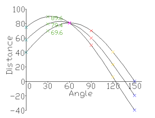
Since the equation of <math>y_i = a x_i + b</math> cannot capture vertical lines (a being the slope, and b being the intercept), Hough transform uses polar coordinates to represent the lines that go through <math>(x_i, y_i)</math>. Basically, the algorithm finds the family of all the possible lines that pass through a point <math>(x_i, y_i)</math> , plots their respective <math>(r_i, \theta_i)</math> in the Hough space, and then looks for the minimum number of intersections needed to detect a line where a threshold has to be tuned, as seen in the figure on the right below. | |||
[[File:Hough.png|400px|thumb|right| Hough Space.]] | |||
[[File:Hough 1.jpg|600px|thumb|center| Hough Space.]] | |||
In OpenCv there exist two functions related to Hough transform, | |||
1. Classical Hough transform. | |||
2. Probabilistic Hough transform. | |||
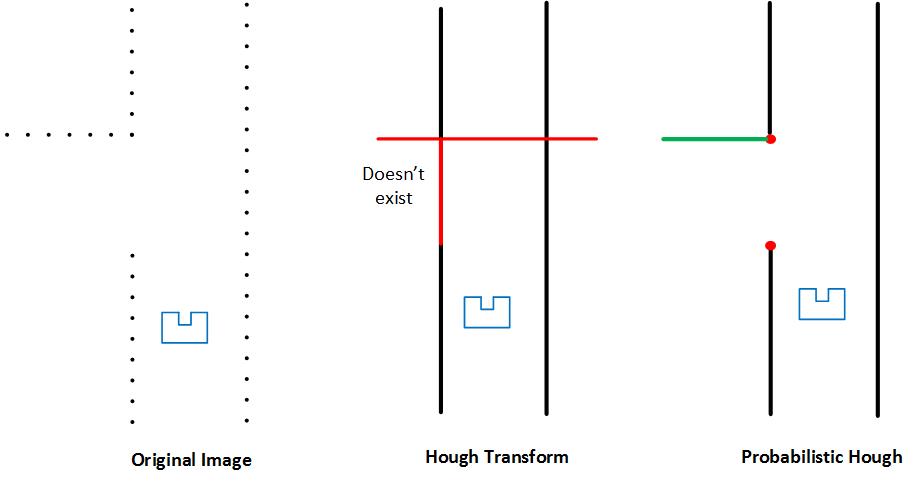
The main difference (in this context) between the two is that probabilistic Hough transform ignores empty pixels. The idea is expressed in the figure above. | |||
However, the output of the probabilistic Hough transform is very noisy giving duplicate and redundant lines which for our purpose is not efficient. As a result, the use of a filter is required. The filtering consists of comparing the output lines by looking at each <math>(r_i, \theta_i)</math> , the ones with the same <math>(r, \theta)</math> are checked and then only the longest one is kept. | |||
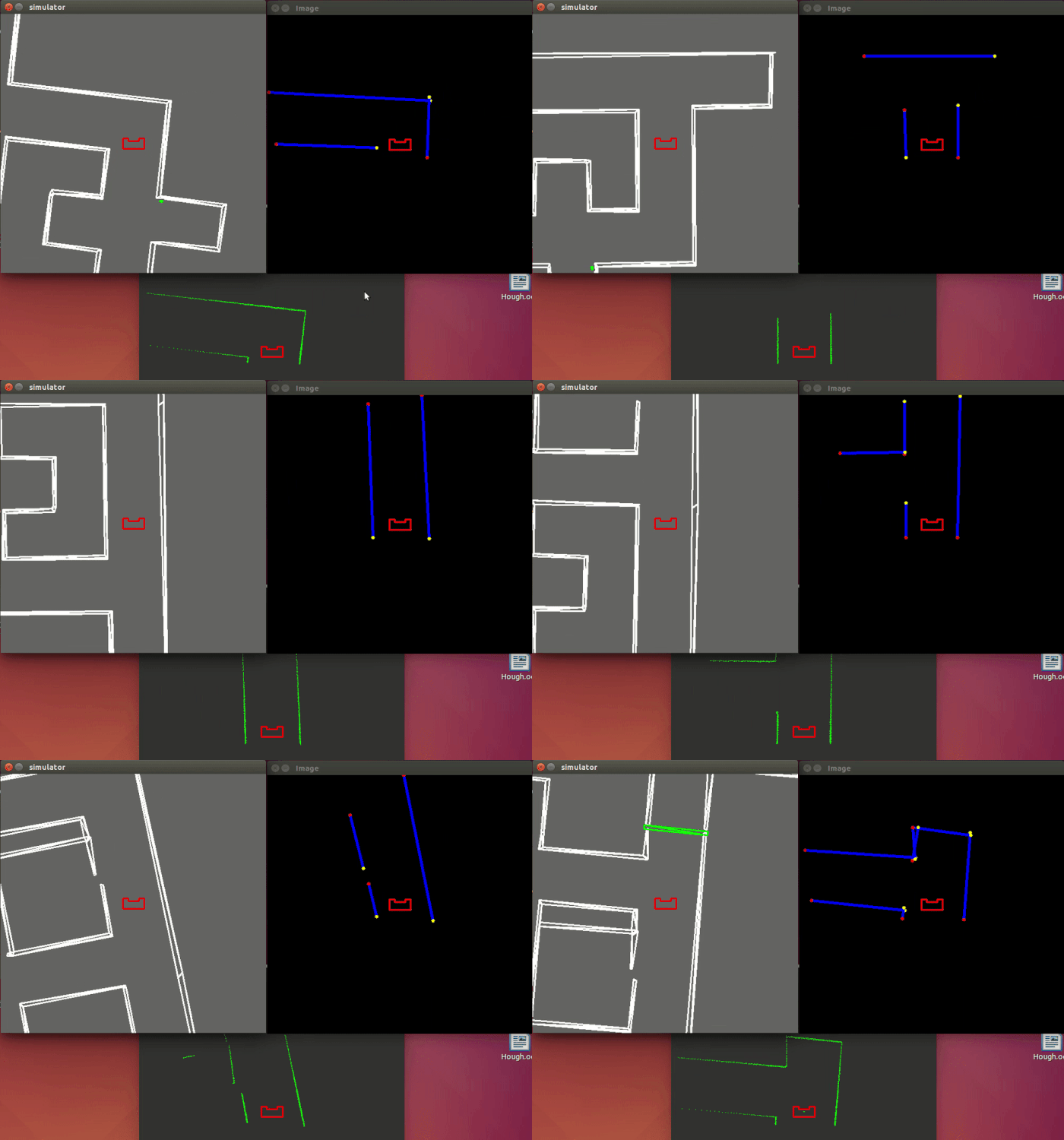
Despite this effort, the result was not what we expected (clean and single lines). However the filtering was able to remove almost 60% of the duplicate lines, but it is not enough to detect all the patterns (turns, junctions) accurately as the Hough lines keep changing. Therefore, this method would be very hard to be used to deliver setpoints for the Potential Field Method. | |||
The idea was eventually abandoned, but the time spent on it did not go to waste because it was very helpful to have the visualization of the robot for testing purposes. | |||
A simulation of the Hough Transform while PICO moves throughout a maze, is shown below. | |||
[[File:Ezgif.com-resize (1).gif|200px|frame|center|Visualisation of the map through the Hough Transform]] | |||
===Detection Circle=== | ===Detection Circle=== | ||
| Line 277: | Line 315: | ||
===Final Simpler Detection=== | ===Final Simpler Detection=== | ||
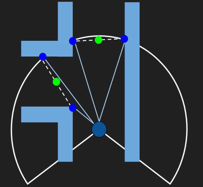
The new, simple detection keeps the idea of the circle of a specific radius, where every laser measurement that is outside of it is discarded. The radius is shortened to 1 m, as a <u>small door</u> at the very small distance of 30cm can be put inside a wall in the maze and this door needs to be identified. This is something that indeed happened on the day | The new, simple detection keeps the idea of the circle of a specific radius, where every laser measurement that is outside of it is discarded. The radius is shortened to 1 m, as a <u>small door</u> at the very small distance of 30cm can be put inside a wall in the maze and this door needs to be identified. This is something that indeed happened on the competition day where our robot was one of the two groups who managed to "spot" the door. | ||
In this method, the following 3 checks are made: | In this method, the following 3 checks are made: | ||
* If 150 laser beams "jump" outside the circle in the range of the laser beams’ numbers 50-350, then PICO detects a right turn. | * If 150 laser beams "jump" outside the circle in the range of the laser beams’ numbers 50-350, then PICO detects a right turn. | ||
| Line 284: | Line 322: | ||
As the reader can conclude, this is a very simple idea, but at the same time, so effective. The only drawback of this idea and especially the use of a shorter radius is that there is a chance in big corridors (around 1.5m) for PICO to detect a "fake" turn. The best solution would be to keep the radius of 1.3m and make a separate function that looks for a small door. But with all the drastic changes that took place in our code over the last few days before the competition, reducing the radius was a quick and quite effective solution to tackle the problem of the small door. | As the reader can conclude, this is a very simple idea, but at the same time, so effective. The only drawback of this idea and especially the use of a shorter radius is that there is a chance in big corridors (around 1.5m) for PICO to detect a "fake" turn. The best solution would be to keep the radius of 1.3m and make a separate function that looks for a small door. But with all the drastic changes that took place in our code over the last few days before the competition, reducing the radius was a quick and quite effective solution to tackle the problem of the small door. | ||
===Dead Ends=== | ===Dead Ends and Doors=== | ||
A dead end can be described as a corridor with a wall in front of PICO. Following this idea we follow this rubric: | |||
* The sum of the distance of the side beams of Pico namely (d1 and d2) are checked if they are within the bound of the corridor max width. | |||
* The front beam (d3) is checked if it is less than 0.7. This number was decided so that Pico can have enough space to make the turn. Also, d1 and d2 should be greater than 0.15 for the same aforementioned reason. | |||
* To avoid detecting inside corners as dead ends, d3 is checked if it’s less than these 4 additional beams (d4, d5, d6 and d7). | |||
The following picture displays this idea. | |||
[[File:Deadendgp3.jpg|700px||thumb|center|Dead end detection]] | |||
Because every dead end is a potential door, Pico rings the bell and waits for 5 seconds and then checks again. If the dead end is a door the above 3 conditions will change to false and thus Pico moves forward. Otherwise, it is indeed a dead end and Pico makes a 180 degree turn, by the use of odometry data and move back into the junction to take another decision. | |||
Below the two scenarios of "dead end" are depicted. In the following left gif, it is indeed a dead end, so the robot turns 180 degrees and moves to another direction. In the following right gif, PICO detects a door and drives through it, once it's open. | Below the two scenarios of "dead end" are depicted. In the following left gif, it is indeed a dead end, so the robot turns 180 degrees and moves to another direction. In the following right gif, PICO detects a door and drives through it, once it's open. | ||
[[File:Door opening.gif|400px|right| | [[File:Door opening.gif|400px|right|frame|PICO detects a dead end again, waits 5 sec to check if it's a door and since the door is open, PICO drives through it.]] | ||
[[File:Dead end.gif|400px| | [[File:Dead end.gif|400px|frame|center|PICO detects a dead end, waits 5 sec to check if it's a door and then it turns 180 degrees and drives to another direction]] | ||
| Line 302: | Line 351: | ||
===Open Spaces=== | ===Open Spaces=== | ||
When PICO is in an open space, it has to follow the closest wall. The way that this is achieved is explained in the <u>Virtual Wall's</u> part. Below the reader can see a simulation of the movement of PICO in an open space. | |||
There are three cases where PICO can run into open spaces and they are shown in the figure below. | |||
[[File:Open space.jpg|700px||thumb|center|Open Space Detection]] | |||
In each case, we assume the existence of an open space and then the beams w.r.t each case are checked (see the figure below). If one of the beams is less than 1.5 which is the corridor max width then it’s not an open space, otherwise it is. | |||
When PICO is in an open space, it has to follow the closest wall. The way that this is achieved is explained in the <u>Virtual Wall's</u> part. Also after the open space PICO must take the next turn of the same direction as the wall it's following. If it's following the right wall, it has to take the next right turn to exit the open space, otherwise the next left turn is required to be taken. Below the reader can see a simulation of the movement of PICO in an open space. | |||
[[File:Open Space.gif|200px|center|frame|PICO detects an open space and starts following the closest wall, in this case the right.]] | |||
===Virtual Walls=== | ===Virtual Walls=== | ||
| Line 319: | Line 377: | ||
In case of a right turn, all laser beams between 650 and 999 are blocked with the same small distance for the whole duration of turning and so a virtual wall is built on the left, which "pushes" PICO to the right. | In case of a right turn, all laser beams between 650 and 999 are blocked with the same small distance for the whole duration of turning and so a virtual wall is built on the left, which "pushes" PICO to the right. | ||
An adjustment of the laser data is also done in the case of the <u>open space</u>. When in open space, the robot checks the distances of the side beams, namely the beams at the 90<sup>o</sup> position (166 and 833). Depending on which one is smaller, the robot follows the corresponding and therefore the closest wall. So the adjustment on the laser measurements is the same as taking a left or a right turn. When the robot has to follow the left wall, all the beams between 0 and 350 are blocked with the same small distance of 0.4 m and when the robot has to follow the right wall, all the beams between 650 and 999 are blocked as well. In both cases, the robot is made to stick to the wall it’s supposed to follow, as it is "pushed" from the virtual wall on its other side. For the simulation of the movement, the reader can take a look at the <u>Open Spaces'</u> part. The function adjust_LRF() can be seen in the snippet below: | An adjustment of the laser data is also done in the case of the <u>open space</u>. When in open space, the robot checks the distances of the side beams, namely the beams at the 90<sup>o</sup> position (166 and 833). Depending on which one is smaller, the robot follows the corresponding and therefore the closest wall. So the adjustment on the laser measurements is the same as taking a left or a right turn. When the robot has to follow the left wall, all the beams between 0 and 350 are blocked with the same small distance of 0.4 m and when the robot has to follow the right wall, all the beams between 650 and 999 are blocked as well. In both cases, the robot is made to stick to the wall it’s supposed to follow, as it is "pushed" from the virtual wall on its other side. For the simulation of the movement, the reader can take a look at the <u>Open Spaces'</u> part. The function adjust_LRF() can be seen in the '''<u>snippet</u>''' below: | ||
[https://gist.github.com/adityakamath/792a5bbcc79229fa97055f094a2a8e9a Adjusting LRF Data using Virtual Walls] | [https://gist.github.com/adityakamath/792a5bbcc79229fa97055f094a2a8e9a Adjusting LRF Data using Virtual Walls] | ||
| Line 343: | Line 401: | ||
* Lastly, a timer of 5 sec has been put for safety, so in case the robot gets "stuck" in a decision for any possible reason (like a turn that wasn’t made completely for some reason), it can "snap out" of it and make a new decision when 5 sec with no new decision have passed. This time interval is more than enough for a turn and as it was mentioned, the robot keeps making new decisions constantly in the corridor, so the timer is not affecting the function of the robot, when everything is normal. | * Lastly, a timer of 5 sec has been put for safety, so in case the robot gets "stuck" in a decision for any possible reason (like a turn that wasn’t made completely for some reason), it can "snap out" of it and make a new decision when 5 sec with no new decision have passed. This time interval is more than enough for a turn and as it was mentioned, the robot keeps making new decisions constantly in the corridor, so the timer is not affecting the function of the robot, when everything is normal. | ||
The use of the transition flag can be seen in the code snippets in the next two sections: Random Walk and Pledge Algorithm | The use of the transition flag can be seen in the code snippets in the next two sections: '''<u>Random Walk</u>''' and '''<u>Pledge Algorithm</u>''' | ||
===Decision Making - Random Walk=== | ===Decision Making - Random Walk=== | ||
The simplest approach of making decisions in the maze is to make random decisions, which is our first implementation in the software, as | The simplest approach of making decisions in the maze is to make random decisions, which is our first implementation in the software, as it’s the easiest one and it is supposed to be our back-up plan, if our decision-making algorithm fails. According to the "random walk", when PICO faces more than one option to go, it randomly picks one and sticks to it, with the use of the "transition conditions" that were mentioned above. Priority is given in the dead ends and the open space, which are special cases and when detected, PICO must act accordingly and stop everything else it’s currently doing. | ||
The function random_walk() checks all the available options (straight/left/right/dead end/open space) and generally picks randomly one of them, when the "transition conditions" allow it of course. The random choice is being done with the function rand(). There is one precaution which is taken into account and that is that when PICO is in an open space and it follows the closest wall, the next decision it must take in the next junction must be the same as the wall | The function random_walk() checks all the available options (straight/left/right/dead end/open space) and generally picks randomly one of them, when the "transition conditions" allow it of course. The random choice is being done with the function rand(). There is one precaution which is taken into account and that is that when PICO is in an open space and it follows the closest wall, the next decision it must take in the next junction must be the same as the wall it’s following e.g. if it’s following the left wall the next decision must be left. In this way, PICO will make sure that it will get out of the open space which is a very difficult case and will not roam in the open space aimlessly. So if the opposite turn is selected then the function is called again, until an acceptable decision is selected. | ||
The function random_walk() is provided in the following snippet: | |||
The function random_walk() is provided in the following '''<u>snippet</u>''': | |||
[https://gist.github.com/adityakamath/f571aa1136bf3cdb8bca5b76cef5dd07 Random Walk function] | [https://gist.github.com/adityakamath/f571aa1136bf3cdb8bca5b76cef5dd07 Random Walk function] | ||
| Line 360: | Line 419: | ||
===Decision Making - Pledge Algorithm=== | ===Decision Making - Pledge Algorithm=== | ||
The function pledge_alg() is provided in the following snippet: | For the strategy, the pledge algorithm was used to determine PICO’s decisions. The pledge algorithm allows PICO to find the maze exit irrespective of the initial position. The idea is based on using a counter to track PICO’s decisions as follows: | ||
* If the counter is 0, PICO goes straight until it hits an obstacle. | |||
* If right and left are both available and the counter is 0, a random choice is taken and the counter is updated. | |||
* For each right turn the counter is increased by 1, whereas for each left turn the counter is decreased by 1. | |||
* For the case of a dead end, the robot will make a 180 degree turn which means we are taking two consecutive left turns and thus the counter is decreased by 2. | |||
* In an open space, Pico will start following the closest wall while keeping updating the counter whenever taking a right or left turn. | |||
The following animation explains the use of the pledge algorithm as PICO drives through the maze and out of the exit. | |||
The function pledge_alg() is provided in the following '''<u>snippet</u>''': | |||
[https://gist.github.com/adityakamath/7f63ef29a0d63574b7d3e1be0c5a22fd Pledge Algorithm function] | [https://gist.github.com/adityakamath/7f63ef29a0d63574b7d3e1be0c5a22fd Pledge Algorithm function] | ||
| Line 366: | Line 433: | ||
Below, the solving of the maze that was used in the maze challenge with the "pledge" algorithm is depicted. Of course here, every decision is anticipated and it taken based on the counter of the turns, so the maze is solved robustly and not just by luck. | Below, the solving of the maze that was used in the maze challenge with the "pledge" algorithm is depicted. Of course here, every decision is anticipated and it taken based on the counter of the turns, so the maze is solved robustly and not just by luck. | ||
[[File:Pledge animation.gif|100px|right|frame|Pledge Algorithm implementation]] | |||
{|style:"margin: 0 auto;" | {|style:"margin: 0 auto;" | ||
| Line 382: | Line 451: | ||
Two codes were developed for the final maze challenge - one running random walk and the other with the pledge algorithm. Although the main loop for each of the two codes were different, the structure of the code remains the same and is described in the tree below: | Two codes were developed for the final maze challenge - one running random walk and the other with the pledge algorithm. Although the main loop for each of the two codes were different, the structure of the code remains the same and is described in the tree below: | ||
src | |||
| | | | ||
+--- | | grp3_pledge.cpp | ||
| grp3_random.cpp | |||
| | | | ||
| | +--- move_functions | ||
| | | CMakeLists.txt | ||
| motion.h | |||
| motion.cpp | |||
| | | | ||
+--- | +--- detect_functions | ||
| | | CMakeLists.txt | ||
| | | detection.h | ||
| | | detection.cpp | ||
| | | | ||
\--- strategy_functions | |||
CMakeLists.txt | |||
strategy.h | |||
strategy.cpp | |||
The main functional loops of each of the two codes are provided in the following '''<u>snippets</u>''' below: | |||
The main functional loops of each of the two codes are provided in the following snippets below: | |||
[https://gist.github.com/adityakamath/0f8e4b031814e57c10c6aa43a26965d0 Random Walk] | [https://gist.github.com/adityakamath/0f8e4b031814e57c10c6aa43a26965d0 Random Walk] | ||
[https://gist.github.com/adityakamath/f7f39753fc4ada0ca353d42ceb4ae17f Pledge Algorithm] | [https://gist.github.com/adityakamath/f7f39753fc4ada0ca353d42ceb4ae17f Pledge Algorithm] | ||
Other more specific '''<u>snippets</u>''', which can be also found in the sections: '''<u>Potential Fields</u>''', '''<u>Virtual Walls</u>''', '''<u>Decision Making - Random Walk</u>''', '''<u>Decision Making - Pledge Algorithm</u>''' are: | |||
[https://gist.github.com/adityakamath/ed8b2cf67b04d43727223b4fa53a44e8 Potential Fields],[https://gist.github.com/adityakamath/792a5bbcc79229fa97055f094a2a8e9a Adjusting LRF Data using Virtual Walls], [https://gist.github.com/adityakamath/f571aa1136bf3cdb8bca5b76cef5dd07 Random Walk function] , [https://gist.github.com/adityakamath/7f63ef29a0d63574b7d3e1be0c5a22fd Pledge Algorithm function] | |||
==Maze Challenge Evaluation== | ==Maze Challenge Evaluation== | ||
' | On <u>June 8 2016</u> the maze competition took place. The maze that was made for the competition day can be seen below. | ||
[[File:Maze design final challenge.png|400px|thumb|right| Final Maze on June 8 2016]] | |||
Only 1 out of 7 teams managed to finish the maze successfully. Unfortunately our team didn’t manage to complete the maze. We got 2<sup>nd</sup> place as PICO managed to get the furthest in the maze from the 6 remaining teams. The door was quite small so 5 teams didn’t detect the door but our team and the winning team managed to do it. | |||
We had 2 attempts in the maze. The 1<sup>st</sup> was by using the pledge algorithm and the 2<sup>nd</sup> was by using random walk. | |||
Firstly, our <u>1st attempt</u> in the maze, with the pledge algorithm is displayed. | |||
{| | |||
|[[File:Image 6.png|left|250px|link=https://www.youtube.com/watch?v=UmOqIg3xerc]] | |||
|} | |||
Secondly, our <u>2nd attempt</u> in the maze, with the random walk is displayed. | |||
{| | |||
|[[File:Image 4.png|center|250px|link=https://www.youtube.com/watch?v=QVRgjOjMU-U]] | |||
|} | |||
<u>1st attempt's evaluation</u> | |||
Our 1<sup>st</sup> attempt was the least successful as the robot failed to go through the door. PICO must have detected a fake turn at [https://youtu.be/UmOqIg3xerc?t=31s 0.31] and that messed up our counter, which is due to the sacrifice we had to make concerning the detection to be able to detect the small door (reducing the radius of the circle from 1.3 to 1 m). But that was a minor problem. The biggest problem is that PICO seemed to have a difficulty to take the decision for left turns. We attribute that to the detection, namely we believe that left turns were detected too late so PICO was generally going either straight or right and that’s why it keeps going over the big loop after one point in the video. It seems unable to take left turns, even though it should, with the exception of going in the dead end at the start of the run. | |||
One other thing that needs to be mentioned is even if PICO, while going over the big loop of the maze, was able to detect the door on its left, the transition wouldn’t enable him to take the decision to go left. To be more specific, that corridor on the left of the door is too small, so PICO is still turning from its previous right turn and it cannot "snap out" of the previous decision, because 90 degrees are still not completed. So, after letting PICO go around the loop 3 times, we stopped that attempt as there was no point in wasting any more of the total 7 minutes that we had to complete the maze and we moved on to our 2<sup>nd</sup> attempt. | |||
<u>2nd attempt's evaluation</u> | |||
In our 2<sup>nd</sup> attempt, PICO was taking random decisions as to whether it’d go straight, right or left. The door was successfully detected this time and PICO stopped right in front of it and "beeped" and the door opened. PICO went through the door but just before it got into the open space, it took the "wrong" decision of going left into the dead end. That was totally random of course but that decision really costed us the successful completion of the maze. If PICO had taken the decision to go right there, then we would have won the maze challenge for sure. After the dead end, PICO had 1 last chance to "rectify" it’s "mistake" by going straight into the open space but instead of that it went right and back into the starting area. | |||
After a point, PICO started to act really weird. | |||
After a point, PICO started to act really weird. As we can see in [https://youtu.be/QVRgjOjMU-U?t=1m39s 1.39], PICO stops in front of the dead end and then, while turning and before completing the 180 degrees’ turn, it moves away and then freezes. This is totally unexpected as it literally freezes, because it’s not that it detected the dead end again, because it didn’t "beep" as it’s supposed to do. After that, it starts going backwards, which is also something that has never happened in the simulation and it crashes and our attempt stops there. | |||
We are not clear about what caused this totally irregular behaviour, as it is repeated, this series of actions are not supposed to take place in any case. So the only logical thing we can conclude is that our software "crashed", PICO lost control and it just drove backwards, stopped for a couple of seconds and then drove backwards again until it crashed. We even tried to replicated the same scenario of movement in the simulation, but this unexpected behaviour never occurred. | |||
=Lessons learnt= | =Lessons learnt= | ||
From this project a lot of experience was drawn, which is summed up to the following lessons: | |||
* Good organization in a project done by 5 members is top priority. During this course, we shifted from one idea to another constantly, at times even tried to implement the same objective with 2 different methods, until we finally settled to our final implementation. This was something devastating, because a lot of valuable time was wasted, which had it been invested better, we are confident we would have won or at least finished the maze competition. So to the <u>future groups</u> doing this course we <u>advise</u>: pick roles from the start, study very well your objective, before you start programming '''but''' at the same time don’t get lost on difficult theoretical ideas for too long, because it’s a practical application and putting your idea to the test is not easy at all. And most importantly: <u>divide tasks and update with the team at least bi-weekly!</u> | |||
* Simulation and test on the robot are 2 different things. While the simulation is pretty accurate and with a good maze map, one can pretty much understand what to anticipate from the actual implementation, testing on the robot can bring up problems that one cannot spot during the simulation. Starting from small things like tuning a gain on the robot is much more accurate to achieve the desired result than the simulation and going to more important stuff like different reaction of the robot in reality in comparison to the simulation. As a team, we encountered at least 2 times a different behaviour on the robot, with code that was working perfectly on the simulation and we had to fix it during the test. So the practice is: | |||
** code, | |||
** simulate, | |||
** despair, but only briefly, | |||
** code more, | |||
** simulate more, | |||
** test | |||
** repeat | |||
* Discarding data is of key importance. Either this is achieved by not receiving data constantly by the use of communication (events) either, as in our case, discarding measurements that are bigger than a specific threshold (detection circle), this principle makes coding much more efficient and effective. This is also one of the lessons that were taught by <u>Herman Bruyninckx</u> during the lectures. | |||
* After the maze competition, we conclude that despite our detection method was satisfactory, it was not perfect. The problem is that depending on the location of the robot, if it is for instance slightly turned to the right, as it’s approaching a junction, not all available ways to choose are visible at the same time. That means that for instance in some cases in a crossroad, the left turn is detected sooner than the right turn and so the robot is not "free" to choose the best decision (left, straight or right) depending on the algorithm used. That can even cause problems if "random walk" is used, because at a specific point that PICO must take for instance the right turn, by not detecting it, the opportunity of even picking that turn randomly is not given to the robot. Therefore, if we had something that we would improve on our software at the end of this course, it would definitely be the detection. | |||
=Good times= | =Good times= | ||
And lastly, to | And lastly, to draw a conclusion on this wiki page on a happy tone, here is a video through the eyes of PICO, | ||
{| | {| | ||
|[[File:Image 24.png|right|250px|link=https://www.youtube.com/watch?v=ar6UCUKMK-k]] | |[[File:Image 24.png|right|250px|link=https://www.youtube.com/watch?v=ar6UCUKMK-k]] | ||
|} | |} | ||
a picture of our desk after a hard and sleepless "emc" night | |||
[[File:47b14cb2-72ab-42fe-aedd-fe89a7a8a6d8.jpg|center|500px|]] | |||
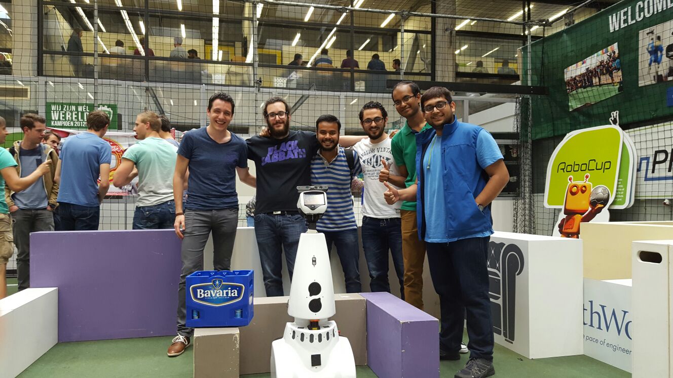
and below a picture of our group with our tutor Yanick and PICO, just after the maze competition. | and below a picture of our group with our tutor Yanick and PICO, just after the maze competition. | ||
[[File:Group 3 with tutor.jpg|center|800px|]] | [[File:Group 3 with tutor.jpg|center|800px|]] | ||
Latest revision as of 13:35, 9 May 2017
Group Members
| 0976155 | Aditya Kamath | a.kamath@student.tue.nl |
| 0980790 | Alexis Siagkris-Lekkos | a.siagkris-lekkos@student.tue.nl |
| 0976940 | Amrith Vel Arul Kumar | a.v.arul.kumar@student.tue.nl |
| 0976467 | Ayush Kumar | a.kumar.1@student.tue.nl |
| 0978245 | Mahmoud Al Abbassi | m.alabbassi@student.tue.nl |
| Tutor | Yanick Douven | y.g.m.douven@tue.nl |
Initial Design Idea
Here the first approach to the problem is presented, namely Design Document 1 that describes the initial design idea for a robot that navigates through a maze and finds the exit autonomously.
Overview
This article presents a summary of the software design to solve the following challenges with the Pico robot.
- Corridor competition: To follow a corridor and take the first exit.
- Maze competition: To solve and exit an unknown maze.
The project is divided in the following aspects:
- Requirements
- Specifications
- Functions
- Components
- Interfaces
Requirements/Specifications
For the brainstorming phase, the requirements and specifications are described in one section as the specifications cannot be determined without an introduction to the robot hardware. The requirements of the robot are as follows:
- The robot should not stand still for more than 30 seconds
- The robot should not collide with the walls
- The robot should solve the undisclosed maze and exit within 5 minutes
- The software should store the maze as a map and the robot should be able to revert back to the last known state/position in case of any error.
- The robot should be able to distinguish between the door and dead ends and send out a request to open the determined door
- The robot should determine if the maze is solved and should stop accordingly
- The optimal exit angle should be calculated (how much wheel actuation is necessary for the turn)
Functions
Functions are divided into low, mid and high level. High level functions are not required for corridor challenge.
Low level
| initialization: | Initialization of sensors, actuators |
| read_inputs: | Read laser (LRF) and encoders (walls as reference) |
| drive_forward: | accelerate, decelerate can be separate sub-functions |
| drive_sideways: | Motor control for sideways motion |
| left_turn: | Turn 90o left( doesn’t necessarily need to be at standstill) |
| right_turn: | Turn 90o right |
| U_turn: | Turn 180o left |
| standstill: | Stay at the same position with zero speed, for instance when it waits for the door to open |
Middle level
| get_distance: | Measure the distance to an obstacle (wall, door, anything) |
| avoid_collision: | Keep a safety distance from walls (possible sub-functions: slow down when you\’re close, completely stop when you\’re ready to crash) |
| kill_switch: | Polling for the manual switch to shut the robot, when needed by us |
| finishing_line: | A function to identify the finishing line and shut down the robot (possible options: use kill-switch or detection of being far away from any wall i.e. no walls in front or to the right/left) |
| find_gaps: | Identify all possible passages, corridors (straight, right, left), identify crossings |
| dead_end: | Identify a dead end and make a U-turn or return_to_last_crossing |
| return_to_last_crossing: | If the robot meets a dead end (this may be integrated into the decision routine) |
| door_check: | Check if there is a door at a dead end ( possibly just check for height is enough, because the doors are shorter than the walls OR just ask for door to open and wait to see if it gets a response) |
High level
| opt_decision: | The robot decides what its next move (move forward, turn, stand still) will be, based on the chosen algorithm for the optimal decision for the maze (algorithm will be decided later on, possible algorithms: A*, Tremaux), on the mapping and on the current position (recognize scenario e.g. Dead end) |
| reference_path: | Create the desired path for the robot, from one point to another (especially for cases that we know exactly where the robot must go, already mapped paths) |
| random_decision: | Take a random decision the first time the robot is at a junction |
| mapping: | Build a map according to the obstacles(walls) or empty spaces (passages, corridors) identified by the laser |
| check_position: | Check if the robot has already been in this position, otherwise store position (starting point=reference point) |
| store_position: | Store the current location of the robot in the map (if not already stored), to create a path and to avoid visiting same places twice |
Components
The PICO robot consists of multiple components which are listed below:
- Sensors:
- Laser Range Finder (LRF): Through the LRF on the PICO one can detect the distance to an object.This is accomplished by sending a laser pulse in a narrow beam towards the object and measuring the time taken by the pulse to be reflected on the target and returned to the sender.
- Wheel encoders (odometry): The encoders will provide us with the speed of the wheels which can be used to control PICO based on the provided data.
- Actuators:
- Holonomic base with omni-wheels
- Pan-tilt unit for head
- Computer
- Intel I7
- Ubuntu14.04
Interfaces
This section describes the interfaces between the following abstractions:
- Challenge context: Describes the goal of the challenge
- Environment context: Describes the environment sensed by the robot
- Robot context: Describes the robot hardware and sensor readings
- Skill context: Describes the robot’s skill-set
- Task context: Describes the decision-making abstraction
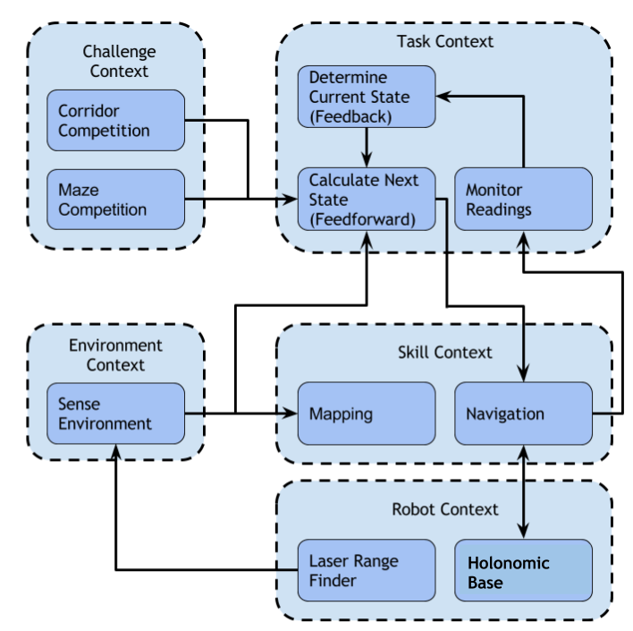
The interfaces between the above abstractions can be seen in the diagram below:
-
Flow chart of the initial software design
Corridor Competition
The Corridor Mission
In the corridor competition, the robot must drive through a corridor, detect the first exit and then take it. The precise location and the kind (right or left) of this exit is not known in advance. For this challenge, a simple method was implemented. The robot uses its laser data (LRF) to navigate through the corridor and its odometry data to make the 90o turn. Then it drives straight into the turn and when the robot is out of the corridor, the robot is immobised and the program is ended.
Alignment with the walls
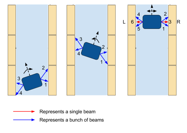
Firstly, the robot makes sure that it’s heading straight towards the end of the corridor so that it doesn’t drive into any walls. In order to do so, it compares an equal bunch of beams in front and behind of the middle side beams, which are the beams at the +-90o of the robot. As we can see in the figure below, there are 3 possible scenarios, heading left, heading right and heading straight. By checking the figure, it can be seen that if the total distance of the bunch of beams with the number 2 is bigger than the distance of bunch 1 and at the same time the distance of bunch 4 is bigger than bunch 3, that means that the robot is facing the left and it needs to turn with a clockwise rotational speed. If the total distance of bunch 2 is smaller than bunch 1 and at the same time the distance of bunch 4 is smaller than bunch 3, then the robot is facing the right and it needs to turn with a counter-clockwise rotational speed. If the aforementioned corresponding bunches of beams are equal then the robot is facing straight and so the rotational speed is 0. At all times the robot is moving forward (x axis) with a constant velocity.
Keeping the robot in the middle of the corridor
The robot is checking the middle side beams, mainly the beams at the +-90o of the robot along with an equal amount of beams in front and behind of them. Basically, only the side beams are needed for keeping the robot in the middle, but more beams are accumulating to make sure that this goal is achieved. In case the total distance of the right bunches of beams (bunch 1, 2 and beam 3) is bigger than the total distance of the left bunches of beams (bunch 4, 5 and beam 6), the robot moves sideways (y axis) to the right. In case the total distance of the left bunches of beams is bigger than the total distance of the right bunches of beams, then the robot moves sideways (y axis) to the left. In case these distances are equal, then the robot is in the middle of the corridor and it doesn’t move sideways so the translational speed in the y axis is 0. In all the above cases, the robot keeps moving straight (x axis) with a constant velocity. All these are depicted in the following figure.
-
Aligning of the robot in the middle
Finding the gap
In order to identify the turn, the robot checks for a big "jump" in the laser measurements, namely a very big difference of the distances returned by two consecutive beams. If this occurs for a specific amount of times (e.g. 20 times), thinking that we may have a small crack in the wall or just a wrong measurement, then it is identified as a turn. Depending on the number of the beam, in which the "jump" is detected, the turn is detected as right or left. So if the number of this beam is smaller than 500, which is the middle beam (the one facing straight of the robot), then the turn is right, otherwise it’s left. After that, the robot calculates the middle of the gap and drives straight until it reaches that point, where it stops. The only difference in this movement is that the robot is following the opposite wall from the turn, keeping a distance from it which is the same as the robot had while moving through the corridor.
Taking the turn
When the robot has stopped, it turns exactly 90o to the right if it’s a right turn or to the left if it’s a left turn. This turn is achieved by checking the odometry data, as they are pretty accurate for just a turn at least and keep turning with a constant rotational speed with the right direction, depending on the turn.
Drive straight in the turn
After the robot has made the turn, the original plan was to continue with the same "driving mode" as before in the corridor. But since there are no walls anymore to the sides of the robot, until at least it drives into the turn, this proved to make the robot bump into the corner sometimes. Only when the robot is completely in the "new" corridor, it can align and drive in the center of the corridor. So a last-day change was made, which makes the robot drive straight in the turn, just by checking if it’s aligned correctly so that it heads towards the exit of the corridor. Of course, a function that prevents the robot from bumping into the walls is also implemented. In this way, it’s been made sure that no bumps occur, because this cancels the attempt and it’s also helping the robot correct its trajectory.
Collision avoidance
A function is implemented that checks all the laser beams and if any of the measurements returns a distance smaller than a specific distance (0.3 m), then the robot moves towards the exact opposite direction of the obstacle. In this way, it’s been made sure that the robot doesn’t drive into a wall and also it helps the robot to fix its trajectory into the corridor.
Exiting the corridor
Another function is implemented which checks all the laser data and if all the laser data detect nothing in a distance of 1 m, this means that the robot has exited the corridor. Then, the robot is immobilised and the program is ended.
Check for invalid LRF
Lastly, a check is being made for invalid LRF, so if a measurements is bigger than a specified range (3.5 m) then it is perceived as invalid and it’s replaced by a small negative value in the scan.ranges array.
The movement in the corridor, step by step, is depicted in the following figure.
-
Movement in the corridor
Our presentation for the corridor was given on May 11 2016.
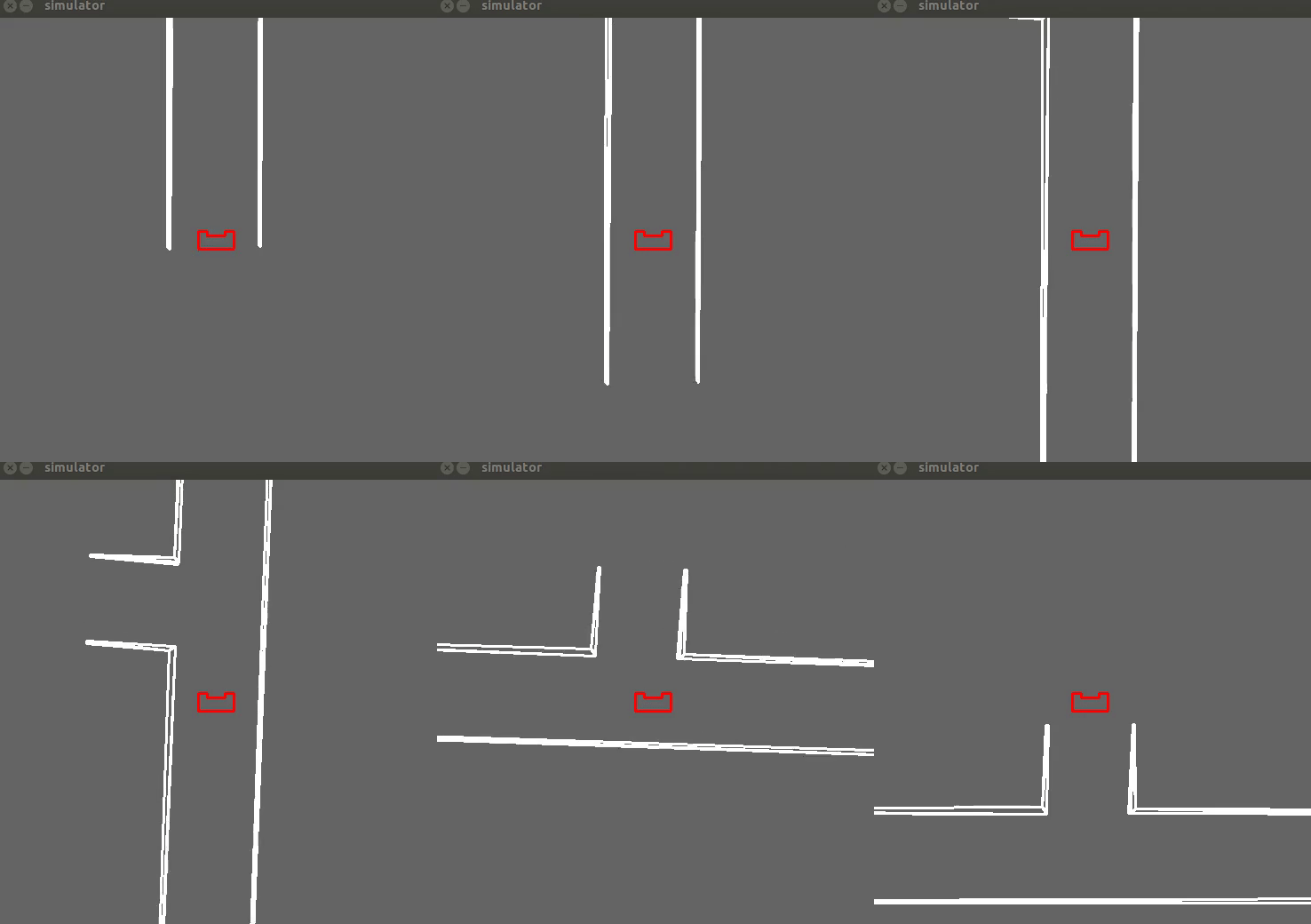
A simulation of the corridor competition is presented below.
Corridor competition evaluation
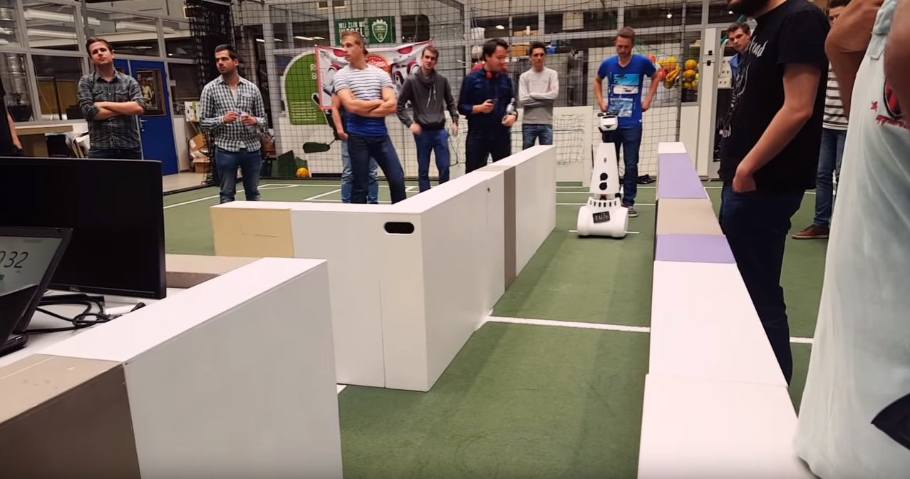
The corridor competition, which the reader can view in the video below, took place on May 18 2015 and our robot was pretty successful. Our team finished namely at the 2nd place with a time of 17 sec, whereas the winning team finished the corridor in 14.5 sec. Many tests were made with different widths of the corridor, even small cracks in the wall and misaligned walls and the robot completed successfully all these routes, so it had no problem completing the corridor challenge. The only disadvantage were the fast changes in the speed, as no PID controller was used, which made the robot vibrate and move around the middle line of the corridor. It needs to be stressed, that despite finishing the competition successfully, this software is not sufficient for the maze competition. So more complex ideas need to be implemented for the maze and more complex methods as Hough transform and potential fields and of course building a much more complete software in order to have a chance of finishing the maze successfully.
 |
Maze Competition
The Maze Mission
In the maze competition, the objective is quite straighforward. PICO must find the exit fully autonomously as quickly as possible. In the maze, dead ends exist, at least one open space, and a door in front of which PICO must ring the bell, in order for it to open and so the robot can continue its way through the maze. PICO cannot tell the difference between doors and dead ends, because to it they're the same thing, just 1 wall in front of it and 1 wall on each side. That means that it has to "beep" in front of every "dead end", wait for 5 sec and then check again if the path is clear. If it is, then it continues, otherwise it turns around.
Software Architecture
General layout
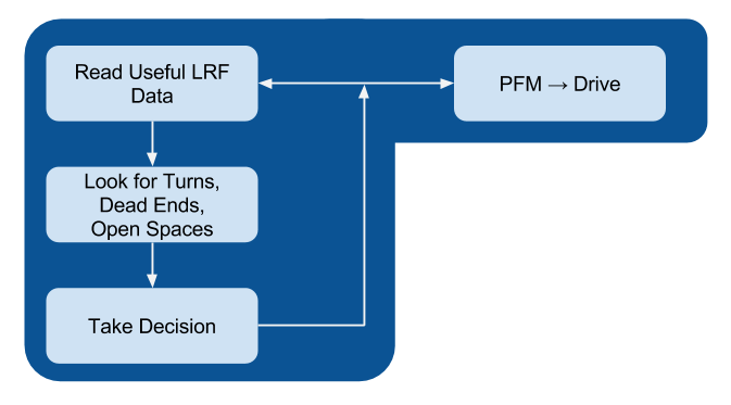
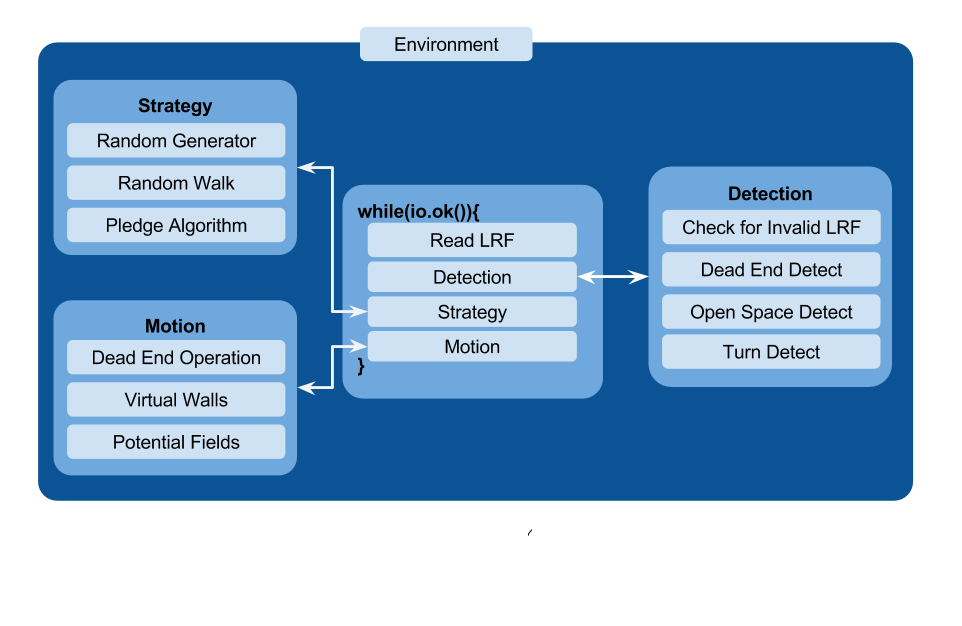
The scope of the challenge was divided into three subsystems:
- Motion
- Detection
- Strategy
The set of functions the make up the Detection subsystem perform the following operations:
- Set a maximum range for laser data
- Look for left/right/straight paths
- Look for dead ends and open spaces
The strategy subsystem uses these detection functions and makes a decision for the robot’s next move.
The motion subsystem drives the robot using potential fields according to the decision made.
The main functional loop utilizes these subsystems as described in the following two flowcharts.
Potential Fields
In order for the robot to drive smoothly through the maze, the previous simple method of driving was deemed inadequate. As mentioned above, that was already known before the corridor challenge, but there was not enough time to implement something more elegant and more effective for the corridor. For the maze, the Potential Fields’ Method was implemented, which was popular among the other teams as well. The basic idea is that virtual repulsive forces are applied to the PICO for every laser point, which push the robot away from the obstacles/walls and one single virtual attractive force towards the setpoint, namely the desired destination, is applied to it. The repulsive forces are very big when the robot is close to an obstacle and smaller when it’s in a safe distance and the exact opposite is true for the attractive force, which is bigger for big distances and smaller for small distances. Therefore, when the sum is taken over all the repulsive forces, the total repulsive forces points away from the close obstacles and by adding the attractive force PICO drives to the desired position, while making sure that it doesn’t bump into walls. Because of the "safety" that the potential field method provides, no function for collision avoidance is used, as it was done for the corridor competition.
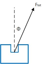
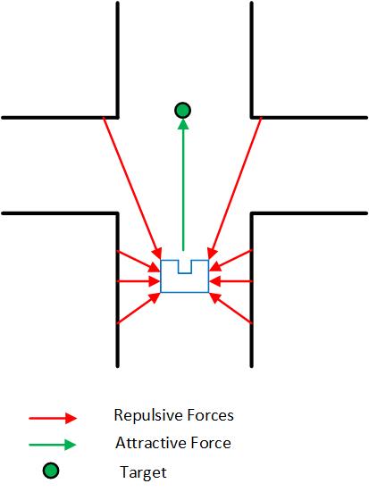
In more details, for every laser measurement, a virtual force is created to the opposite direction of every measurement and a virtual force in the direction of the setpoint is also created. Different weights are used for the repulsive forces and the attractive one as well as for the translational x,y velocities and the rotational w velocity. The total virtual forces in the x and the y direction are calculated separately and the corresponding forces are "translated" to velocities by using a different weight for each one:
[math]\displaystyle{ v_x = w_{vx} * Ftot_{x} }[/math]
[math]\displaystyle{ v_y = w_{vy} * Ftot_{y} }[/math]
As shown in the figure above, the angle of the total force with respect to the 500th beam of the robot, which is the beam pointing to the x direction of the robot, is calculated. This angle is used to calculate the needed rotational velocity, which always tries to make this angle 0 by implementing basically a P controller. In this way, the robot always turns towards the desired direction and the bigger this angle is, the bigger the rotational speed is and so the faster the robot is turning. The type used is:
[math]\displaystyle{ w = w_{w} * \phi }[/math]
At the end of the potential field function, all the velocities are saturated within their limits, the translational x,y speeds to 0.5 m/s and the rotational speed w to 1.2 rad/s. Of course these speeds would be saturated within the robot as well, but in this way consistency is achieved in the simulation and in the experiment as well.
A number of tests were done on the potential field method which are shown in the videos below. In the first one, the collision avoidance skill of the robot is used. No setpoint is used in this case, so the robot just moves to a safe distance away from every obstacle.
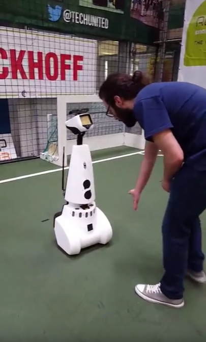 |
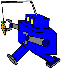
In the second video the robot is put into a maze with only one way to go, so only one option. A very small setpoint of 10 cm ahead is given, just enough to make the robot drive forward, otherwise with no setpoint the robot is just pushed away from the obstacles until it’s in a safe distance, as is seen in the video above. This setpoint serves basically as a "carrot on a stick" to make the robot move forward and when it gets close to any obstacle the repulsive forces make the robot turn away from them so PICO keeps driving forward again until the next obstacle is encountered.
The following video shows that an one-way maze can be solved with no detection of patterns and no actual setpoint, just by almost 30 lines of code which implement the movement around the obstacles.
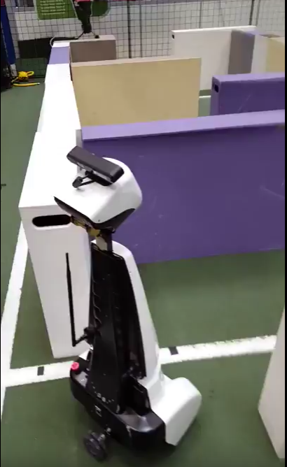 |
Furthermore, a maze which could be solved by a wall-following technique, namely a maze with no loops and no doors, could also be solved by just this small piece of code. All that needs to be added is another small setpoint ("carrot") in the y direction in whichever direction, depending on which wall we want to follow (right or left). Unfortunately no video was recorded of this "capability" of the robot but the reader can view the video attached to the Virtual walls’ section. In this video, virtual walls are used to follow the right wall, which will be explained below, but the result is very similar if one just uses an additional setpoint on the y direction, pointing to the right of the robot. The robot sticks to the right wall, without colliding with it and is able to drive successfully through the maze this way. This shows the "power" of the potential fields’ method, which proves why it’s such a good and important choice for the implementation of the movement.
A snippet of the potential fields function is provided below:
Visualisation - Hough Transform
The LRF data returns a cloud of points. At first, it’s intuitive to look for transforming those points into a comprehensible attribute i.e. lines. For this objective, Hough transform is utilized. Since the equation of [math]\displaystyle{ y_i = a x_i + b }[/math] cannot capture vertical lines (a being the slope, and b being the intercept), Hough transform uses polar coordinates to represent the lines that go through [math]\displaystyle{ (x_i, y_i) }[/math]. Basically, the algorithm finds the family of all the possible lines that pass through a point [math]\displaystyle{ (x_i, y_i) }[/math] , plots their respective [math]\displaystyle{ (r_i, \theta_i) }[/math] in the Hough space, and then looks for the minimum number of intersections needed to detect a line where a threshold has to be tuned, as seen in the figure on the right below.
In OpenCv there exist two functions related to Hough transform,
1. Classical Hough transform.
2. Probabilistic Hough transform.
The main difference (in this context) between the two is that probabilistic Hough transform ignores empty pixels. The idea is expressed in the figure above.
However, the output of the probabilistic Hough transform is very noisy giving duplicate and redundant lines which for our purpose is not efficient. As a result, the use of a filter is required. The filtering consists of comparing the output lines by looking at each [math]\displaystyle{ (r_i, \theta_i) }[/math] , the ones with the same [math]\displaystyle{ (r, \theta) }[/math] are checked and then only the longest one is kept. Despite this effort, the result was not what we expected (clean and single lines). However the filtering was able to remove almost 60% of the duplicate lines, but it is not enough to detect all the patterns (turns, junctions) accurately as the Hough lines keep changing. Therefore, this method would be very hard to be used to deliver setpoints for the Potential Field Method.
The idea was eventually abandoned, but the time spent on it did not go to waste because it was very helpful to have the visualization of the robot for testing purposes.
A simulation of the Hough Transform while PICO moves throughout a maze, is shown below.
Detection Circle
After the abandonment of the idea of using the Hough Transform for detection and for the deliverance of the setpoint, our group moved on to another idea, which was meant to fail as well. In this idea, Laser range finder (LRF) is used to virtually draw a circle around the PICO within a radius of 1.3 meters. This is done by truncating the data above this range and a predetermined threshold is used to constantly check the distance between two consecutive points thereby giving coordinates of those two points, whose midpoint is calculated easily. To make this idea robust enough, the angle between the two detected points is checked and compared with a threshold to solidify the detected points as the points of intersection of the virtual circle with the maze. Checking the above two conditions (distance and angle between the points) help in detecting a valid gap thus making PICO aware of a corridor, left turn, right turn or a combination of the above. Moreover, having these two conditions, a very accurate detection is achieved and cracks in in the wall, which could be mistaken for turns, are ignored. This idea is depicted in the figures below.
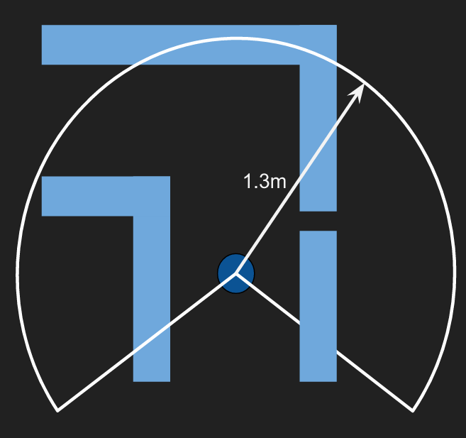
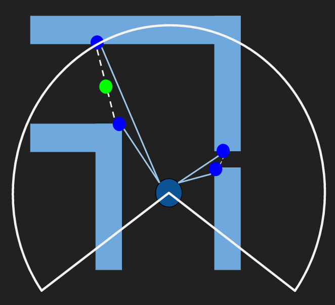
This idea is quite powerful, because it solves the problem of the detection and the problem of setpoints with a combined solution. The easiest scenario is when PICO is driving in the corridor where a midpoint is calculated and is fed to potential function for PICO to drive smoothly to the target. As already stated, this idea is extended on detecting turns and junctions. For example, let’s assume PICO is in the corridor initially and there is only 1 setpoint(mid-point) detected and after a while PICO comes across a left turn, simultaneously 4 pairs of coordinates are detected. Thereby two separate setpoints are passed on to the potential fields and similarly a maximum of 3 set-points can be detected in case of a junction. Moreover, a dead end is detected if no consecutive laser data points show a gap bigger than the threshold value. This idea looks perfect in theory and quite intuitive for PICO to drive in successfully based on the setpoint detection. Unfortunately, the implementation of this started only 2 weeks before the competition and problems were faced mainly in making decisions when PICO sees multiple setpoints and sticking to the selected one. An idea to tackle this is based on comparing the newly detected setpoints each time with the previous ones and calculating the distance from them and then keep on choosing the one with the smallest distance value. This very question of sticking to the selected setpoints was rightly raised by our tutor, Yanick Douven ,during our final presentation as well, which served as an alarm bell of us reevaluating our choices up until this point. Unfortunately, the above idea of detection and setpoints had to be abandoned because it was quite hard to implement and it was replaced by the use of virtual walls, which are explained below. Due to the constant change of plans and ideas for the implementation of the detection and the movement, we reached at a point one week before the maze challenge, which our software was not going to work on time for the weekly test on the robot. So a brave decision was taken overnight and the complicated detection was substituted with a much simpler one, as well as the setpoint idea with virtual walls.
Final Simpler Detection
The new, simple detection keeps the idea of the circle of a specific radius, where every laser measurement that is outside of it is discarded. The radius is shortened to 1 m, as a small door at the very small distance of 30cm can be put inside a wall in the maze and this door needs to be identified. This is something that indeed happened on the competition day where our robot was one of the two groups who managed to "spot" the door. In this method, the following 3 checks are made:
- If 150 laser beams "jump" outside the circle in the range of the laser beams’ numbers 50-350, then PICO detects a right turn.
- If 150 laser beams "jump" outside the circle in the range of the laser beams’ numbers 650-950, then PICO detects a left turn.
- Finally, if 35 laser beams "jump" outside the circle in the range of the laser beams’ numbers 400-600, then PICO detects a gap straight, namely a corridor.
As the reader can conclude, this is a very simple idea, but at the same time, so effective. The only drawback of this idea and especially the use of a shorter radius is that there is a chance in big corridors (around 1.5m) for PICO to detect a "fake" turn. The best solution would be to keep the radius of 1.3m and make a separate function that looks for a small door. But with all the drastic changes that took place in our code over the last few days before the competition, reducing the radius was a quick and quite effective solution to tackle the problem of the small door.
Dead Ends and Doors
A dead end can be described as a corridor with a wall in front of PICO. Following this idea we follow this rubric:
- The sum of the distance of the side beams of Pico namely (d1 and d2) are checked if they are within the bound of the corridor max width.
- The front beam (d3) is checked if it is less than 0.7. This number was decided so that Pico can have enough space to make the turn. Also, d1 and d2 should be greater than 0.15 for the same aforementioned reason.
- To avoid detecting inside corners as dead ends, d3 is checked if it’s less than these 4 additional beams (d4, d5, d6 and d7).
The following picture displays this idea.

Because every dead end is a potential door, Pico rings the bell and waits for 5 seconds and then checks again. If the dead end is a door the above 3 conditions will change to false and thus Pico moves forward. Otherwise, it is indeed a dead end and Pico makes a 180 degree turn, by the use of odometry data and move back into the junction to take another decision.
Below the two scenarios of "dead end" are depicted. In the following left gif, it is indeed a dead end, so the robot turns 180 degrees and moves to another direction. In the following right gif, PICO detects a door and drives through it, once it's open.


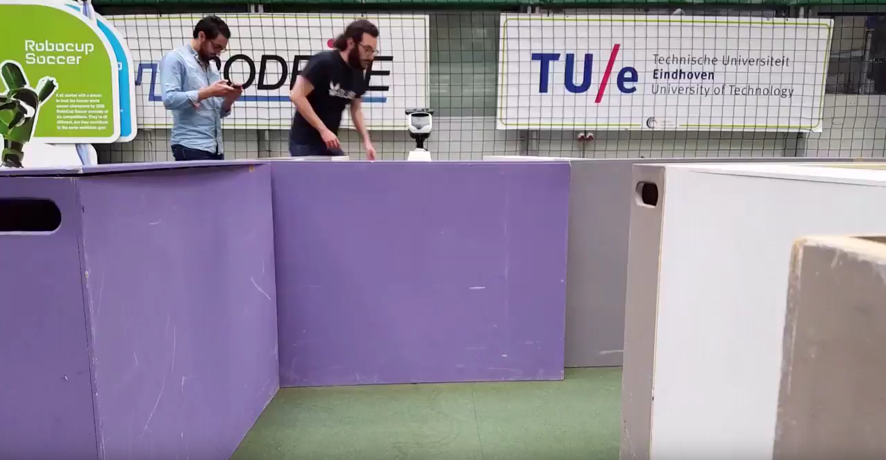
A video from the detection of a door follows.
 |
Open Spaces
There are three cases where PICO can run into open spaces and they are shown in the figure below.
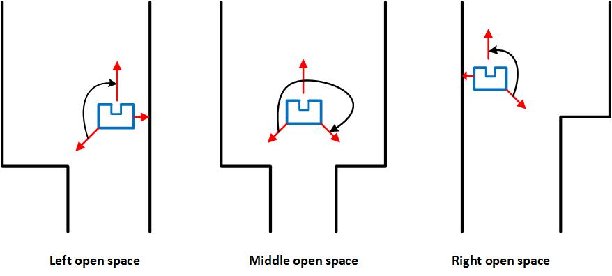
In each case, we assume the existence of an open space and then the beams w.r.t each case are checked (see the figure below). If one of the beams is less than 1.5 which is the corridor max width then it’s not an open space, otherwise it is.
When PICO is in an open space, it has to follow the closest wall. The way that this is achieved is explained in the Virtual Wall's part. Also after the open space PICO must take the next turn of the same direction as the wall it's following. If it's following the right wall, it has to take the next right turn to exit the open space, otherwise the next left turn is required to be taken. Below the reader can see a simulation of the movement of PICO in an open space.

Virtual Walls
As was mentioned earlier, the original idea for the movement of PICO through the maze was to use setpoints. Since that idea was abandoned, the need for setpoints was eliminated by the use of virtual walls. It has already been proven that the robot can move forward avoiding the obstacles, just by providing a very small setpoint in front of it, what we like to call a "carrot on a stick" for the robot. This works perfectly when there is only one way for the robot to go. The idea of the virtual walls takes advantage exactly of this feature. When the robot comes across a crossroad or a T-junction, and it "decides" to go straight, then no action is taken and the robot continues straight with the use of potential fields. In case the robot "wants" to turn right or left, a virtual wall is built on the opposite side of the wanted direction, to make the robot go the other way. This is achieved in the function adjust_LRF(), where the laser measurements are adjusted, depending on the motion the robot is supposed to make. In case the robot is supposed to take a left turn, all the lasers beams between 0 and 350 are blocked with a small distance, namely 0.4 m, for the whole duration of turning. That makes the robot "see" an obstacle on its right, which practically "pushes" PICO to the opposite direction, namely left. This virtual wall is maintained for the whole movement of turning and when the turn is done, the virtual wall is lifted. The following figure makes the use of virtual walls clear.
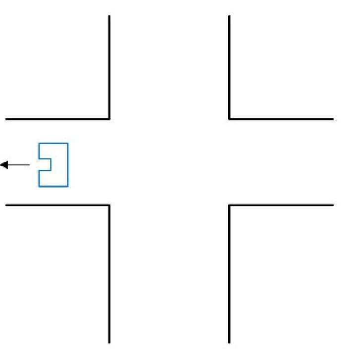
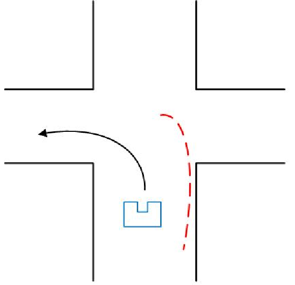
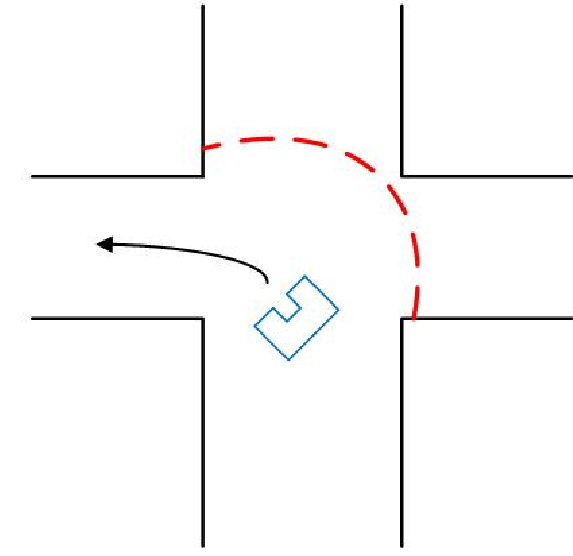
In case of a right turn, all laser beams between 650 and 999 are blocked with the same small distance for the whole duration of turning and so a virtual wall is built on the left, which "pushes" PICO to the right.
An adjustment of the laser data is also done in the case of the open space. When in open space, the robot checks the distances of the side beams, namely the beams at the 90o position (166 and 833). Depending on which one is smaller, the robot follows the corresponding and therefore the closest wall. So the adjustment on the laser measurements is the same as taking a left or a right turn. When the robot has to follow the left wall, all the beams between 0 and 350 are blocked with the same small distance of 0.4 m and when the robot has to follow the right wall, all the beams between 650 and 999 are blocked as well. In both cases, the robot is made to stick to the wall it’s supposed to follow, as it is "pushed" from the virtual wall on its other side. For the simulation of the movement, the reader can take a look at the Open Spaces' part. The function adjust_LRF() can be seen in the snippet below:
Adjusting LRF Data using Virtual Walls
In the following video, the reader can see the effectiveness of the virtual walls in action, in which a simple maze is solved by following the right wall. In this video the laser beams on the left side of the robot are continuously blocked and PICO sticks to the right wall constantly and takes all the right turns, until it's out of the maze.
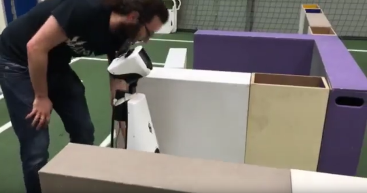 |
Transition Between Decisions
A very important part of the software is the decision making. In other words, when faced with more than one options to go, PICO must pick one, namely pick between the choices: straight, right and left. The same holds for more complicated cases like open space and dead end. But before any reference to the way of making decisions is made, a very important aspect must be explained. When PICO makes a decision, it must stick to it until the movement imposed by this decision is fulfilled. For instance, if the robot "decides" to go right in a crossroad, it must not keep taking new decisions (right/straight/left) while in the junction, just because it has multiple choices to go. If that happens, it’ll either crash on the wall or the decision that must be taken, may not be fulfilled, e.g. if the robot "wants" to go right and it keeps taking new decisions all the time before the right turn is done, it may as well go straight or left or even crash. In order to avoid this, a number of "transition conditions" are taken within the decision-making functions, which will be explained later, just to make sure that when a decision is made, this decision will be followed until the robot is ready to make a new decision. A number of cases/conditions are therefore taken:
- When the robot is turning left, no decision is made until the robot makes a 90o turn to the left.
- When the robot is turning right, no decision is made until the robot makes a 90o turn to the right. In both cases the odometry data are used for measuring the turn.
- When the robot is going straight in a junction, no decision is made until the robot is again within a corridor, after having passed the crossroad. So basically PICO "checks" that it has been in a corridor firstly, then that is has been in the junction and then it has been inside a corridor again.
- While in the corridor, the robot keeps making new decisions, to make sure that when a junction is met, meaning a different option than straight appears, PICO is ready to make a new decision.
All the above conditions are overwritten, when PICO comes across a dead end or an open space, as these two patterns are treated as separate cases. So the "transition conditions" continue as:
- When PICO detects a dead end for the first time, it "snaps out" from every decision it has made and is currently fulfilling, to detect if it’s in front of a door or a dead end, as this is top priority.
- When PICO detects an open space for the first time, it also makes a new decision, as it needs to follow the closest wall (top priority again).
- Furthermore, when PICO is out of the open space it needs to make a new decision once more, so it’s checked if it has been in the open space but it’s not anymore in it.
- Lastly, a timer of 5 sec has been put for safety, so in case the robot gets "stuck" in a decision for any possible reason (like a turn that wasn’t made completely for some reason), it can "snap out" of it and make a new decision when 5 sec with no new decision have passed. This time interval is more than enough for a turn and as it was mentioned, the robot keeps making new decisions constantly in the corridor, so the timer is not affecting the function of the robot, when everything is normal.
The use of the transition flag can be seen in the code snippets in the next two sections: Random Walk and Pledge Algorithm
Decision Making - Random Walk
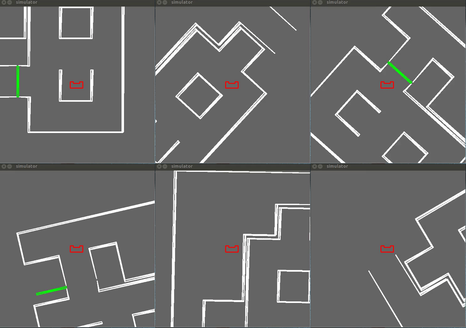
The simplest approach of making decisions in the maze is to make random decisions, which is our first implementation in the software, as it’s the easiest one and it is supposed to be our back-up plan, if our decision-making algorithm fails. According to the "random walk", when PICO faces more than one option to go, it randomly picks one and sticks to it, with the use of the "transition conditions" that were mentioned above. Priority is given in the dead ends and the open space, which are special cases and when detected, PICO must act accordingly and stop everything else it’s currently doing. The function random_walk() checks all the available options (straight/left/right/dead end/open space) and generally picks randomly one of them, when the "transition conditions" allow it of course. The random choice is being done with the function rand(). There is one precaution which is taken into account and that is that when PICO is in an open space and it follows the closest wall, the next decision it must take in the next junction must be the same as the wall it’s following e.g. if it’s following the left wall the next decision must be left. In this way, PICO will make sure that it will get out of the open space which is a very difficult case and will not roam in the open space aimlessly. So if the opposite turn is selected then the function is called again, until an acceptable decision is selected.
The function random_walk() is provided in the following snippet:
Below, the solving of the maze that was used in the maze challenge with the "random walk" is depicted. With the "random walk", as its name states, PICO takes random decisions. In the following gif all the right decisions are taken but that's not necessary. However, if enough time is given to PICO for a small maze, like the final maze, at some point PICO will find the exit anyway.
 |
Decision Making - Pledge Algorithm
For the strategy, the pledge algorithm was used to determine PICO’s decisions. The pledge algorithm allows PICO to find the maze exit irrespective of the initial position. The idea is based on using a counter to track PICO’s decisions as follows:
- If the counter is 0, PICO goes straight until it hits an obstacle.
- If right and left are both available and the counter is 0, a random choice is taken and the counter is updated.
- For each right turn the counter is increased by 1, whereas for each left turn the counter is decreased by 1.
- For the case of a dead end, the robot will make a 180 degree turn which means we are taking two consecutive left turns and thus the counter is decreased by 2.
- In an open space, Pico will start following the closest wall while keeping updating the counter whenever taking a right or left turn.
The following animation explains the use of the pledge algorithm as PICO drives through the maze and out of the exit.
The function pledge_alg() is provided in the following snippet:
Below, the solving of the maze that was used in the maze challenge with the "pledge" algorithm is depicted. Of course here, every decision is anticipated and it taken based on the counter of the turns, so the maze is solved robustly and not just by luck.

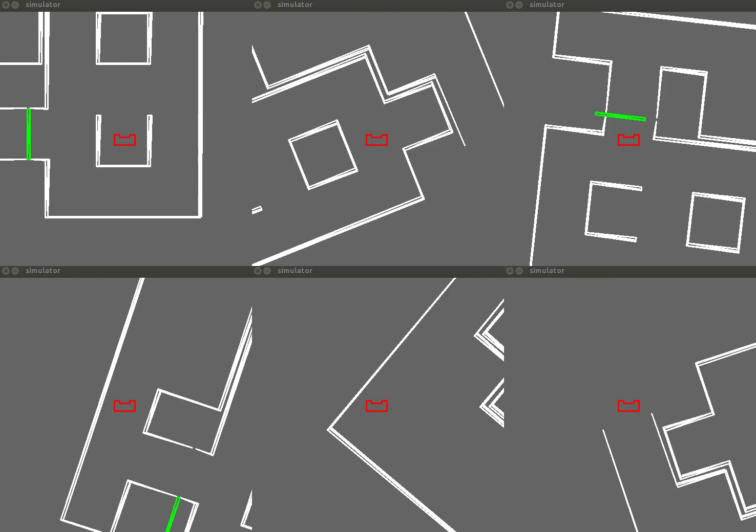 |
Final Presentation, Changes and Improvements
Our presentation for the maze took place on June 1 2016.
This presentation made us see the flaws and difficulties in our design. Since we were forced to make massive changes over the last week before the competition, our final presentation doesn’t quite reflect our final design. The basic changes are the abandonment of Hough transform and the detection circle of radius 1.3m to detect the patterns and calculate the setpoint for the potential field method, as at the time of the presentation the group was trying to approach the same problem with 2 methods (Hough and detection circle) and see which one was working better. The Hough transform, although it didn’t produce the expected results, is not deemed as wasted time, as having made our own visualization was very educative and useful for supervision. As was said earlier, the detection circle method was transformed to a simpler one and virtual walls were used instead of setpoints. Also at that point, we hadn’t even solved the problem of dead ends and open spaces and not even come up with the “transition conditions” between the consecutive decisions of the robot. Finally, the thought at that point was to use “random walk” only as we thought that we wouldn’t have enough time to develop an algorithm to guide us out of the maze, but finally we managed to implement another design with the “pledge” algorithm.
All the above show exactly the disadvantages of not settling on one solution and sticking to it or not picking the best solution right away, which is of course very difficult. On the other hand, they also show the experience derived from all this process and the ability, after all this preoccupation with the project, to achieve massive things in limited time. In other words, we may had reached the final week before we made the final and most important changes in our software but at the same time we managed to deliver a working software and actually achieve the 2nd place in the maze competition.
Code Structure
Two codes were developed for the final maze challenge - one running random walk and the other with the pledge algorithm. Although the main loop for each of the two codes were different, the structure of the code remains the same and is described in the tree below:
src
|
|   grp3_pledge.cpp
|   grp3_random.cpp
|
+--- move_functions
|       CMakeLists.txt
|       motion.h
|       motion.cpp
|
+--- detect_functions
|       CMakeLists.txt
|       detection.h
|       detection.cpp
|
\--- strategy_functions
        CMakeLists.txt
        strategy.h
        strategy.cpp
The main functional loops of each of the two codes are provided in the following snippets below:
Other more specific snippets, which can be also found in the sections: Potential Fields, Virtual Walls, Decision Making - Random Walk, Decision Making - Pledge Algorithm are:
Potential Fields,Adjusting LRF Data using Virtual Walls, Random Walk function , Pledge Algorithm function
Maze Challenge Evaluation
On June 8 2016 the maze competition took place. The maze that was made for the competition day can be seen below.
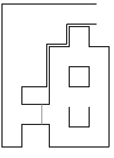
Only 1 out of 7 teams managed to finish the maze successfully. Unfortunately our team didn’t manage to complete the maze. We got 2nd place as PICO managed to get the furthest in the maze from the 6 remaining teams. The door was quite small so 5 teams didn’t detect the door but our team and the winning team managed to do it. We had 2 attempts in the maze. The 1st was by using the pledge algorithm and the 2nd was by using random walk.
Firstly, our 1st attempt in the maze, with the pledge algorithm is displayed.
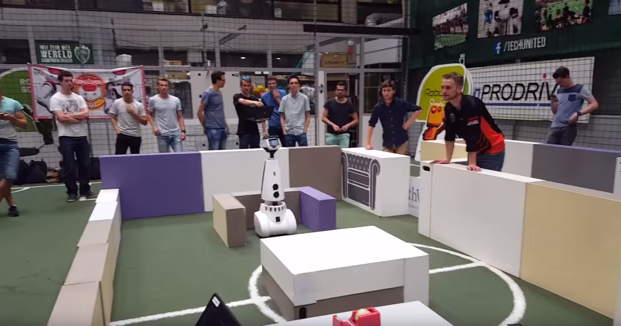 |
Secondly, our 2nd attempt in the maze, with the random walk is displayed.
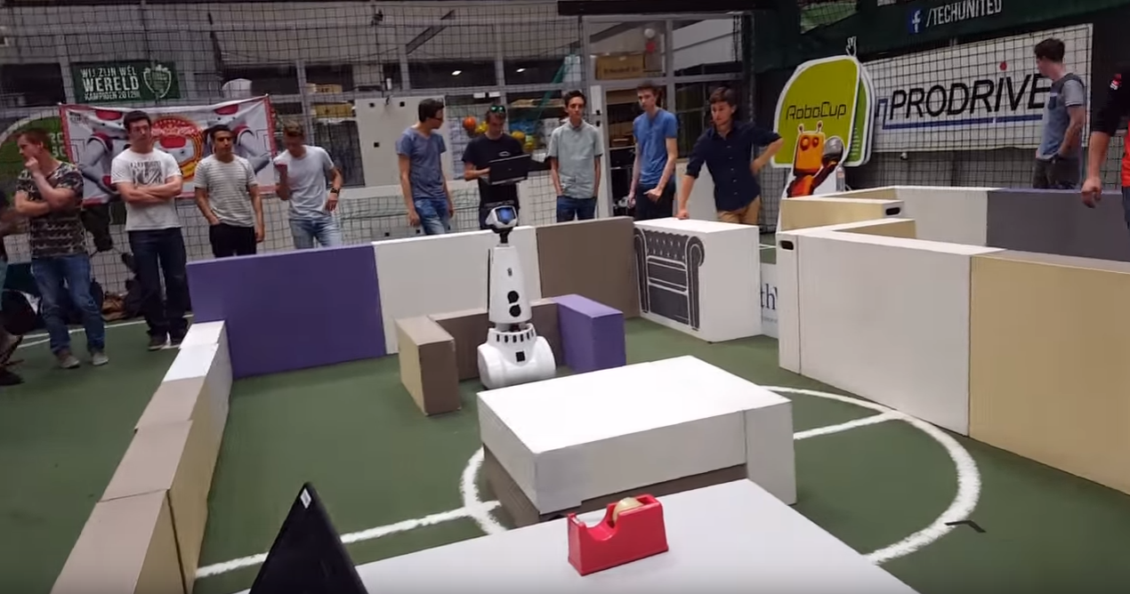 |
1st attempt's evaluation
Our 1st attempt was the least successful as the robot failed to go through the door. PICO must have detected a fake turn at 0.31 and that messed up our counter, which is due to the sacrifice we had to make concerning the detection to be able to detect the small door (reducing the radius of the circle from 1.3 to 1 m). But that was a minor problem. The biggest problem is that PICO seemed to have a difficulty to take the decision for left turns. We attribute that to the detection, namely we believe that left turns were detected too late so PICO was generally going either straight or right and that’s why it keeps going over the big loop after one point in the video. It seems unable to take left turns, even though it should, with the exception of going in the dead end at the start of the run. One other thing that needs to be mentioned is even if PICO, while going over the big loop of the maze, was able to detect the door on its left, the transition wouldn’t enable him to take the decision to go left. To be more specific, that corridor on the left of the door is too small, so PICO is still turning from its previous right turn and it cannot "snap out" of the previous decision, because 90 degrees are still not completed. So, after letting PICO go around the loop 3 times, we stopped that attempt as there was no point in wasting any more of the total 7 minutes that we had to complete the maze and we moved on to our 2nd attempt.
2nd attempt's evaluation
In our 2nd attempt, PICO was taking random decisions as to whether it’d go straight, right or left. The door was successfully detected this time and PICO stopped right in front of it and "beeped" and the door opened. PICO went through the door but just before it got into the open space, it took the "wrong" decision of going left into the dead end. That was totally random of course but that decision really costed us the successful completion of the maze. If PICO had taken the decision to go right there, then we would have won the maze challenge for sure. After the dead end, PICO had 1 last chance to "rectify" it’s "mistake" by going straight into the open space but instead of that it went right and back into the starting area. After a point, PICO started to act really weird.
After a point, PICO started to act really weird. As we can see in 1.39, PICO stops in front of the dead end and then, while turning and before completing the 180 degrees’ turn, it moves away and then freezes. This is totally unexpected as it literally freezes, because it’s not that it detected the dead end again, because it didn’t "beep" as it’s supposed to do. After that, it starts going backwards, which is also something that has never happened in the simulation and it crashes and our attempt stops there.
We are not clear about what caused this totally irregular behaviour, as it is repeated, this series of actions are not supposed to take place in any case. So the only logical thing we can conclude is that our software "crashed", PICO lost control and it just drove backwards, stopped for a couple of seconds and then drove backwards again until it crashed. We even tried to replicated the same scenario of movement in the simulation, but this unexpected behaviour never occurred.
Lessons learnt
From this project a lot of experience was drawn, which is summed up to the following lessons:
- Good organization in a project done by 5 members is top priority. During this course, we shifted from one idea to another constantly, at times even tried to implement the same objective with 2 different methods, until we finally settled to our final implementation. This was something devastating, because a lot of valuable time was wasted, which had it been invested better, we are confident we would have won or at least finished the maze competition. So to the future groups doing this course we advise: pick roles from the start, study very well your objective, before you start programming but at the same time don’t get lost on difficult theoretical ideas for too long, because it’s a practical application and putting your idea to the test is not easy at all. And most importantly: divide tasks and update with the team at least bi-weekly!
- Simulation and test on the robot are 2 different things. While the simulation is pretty accurate and with a good maze map, one can pretty much understand what to anticipate from the actual implementation, testing on the robot can bring up problems that one cannot spot during the simulation. Starting from small things like tuning a gain on the robot is much more accurate to achieve the desired result than the simulation and going to more important stuff like different reaction of the robot in reality in comparison to the simulation. As a team, we encountered at least 2 times a different behaviour on the robot, with code that was working perfectly on the simulation and we had to fix it during the test. So the practice is:
- code,
- simulate,
- despair, but only briefly,
- code more,
- simulate more,
- test
- repeat
- Discarding data is of key importance. Either this is achieved by not receiving data constantly by the use of communication (events) either, as in our case, discarding measurements that are bigger than a specific threshold (detection circle), this principle makes coding much more efficient and effective. This is also one of the lessons that were taught by Herman Bruyninckx during the lectures.
- After the maze competition, we conclude that despite our detection method was satisfactory, it was not perfect. The problem is that depending on the location of the robot, if it is for instance slightly turned to the right, as it’s approaching a junction, not all available ways to choose are visible at the same time. That means that for instance in some cases in a crossroad, the left turn is detected sooner than the right turn and so the robot is not "free" to choose the best decision (left, straight or right) depending on the algorithm used. That can even cause problems if "random walk" is used, because at a specific point that PICO must take for instance the right turn, by not detecting it, the opportunity of even picking that turn randomly is not given to the robot. Therefore, if we had something that we would improve on our software at the end of this course, it would definitely be the detection.
Good times
And lastly, to draw a conclusion on this wiki page on a happy tone, here is a video through the eyes of PICO,
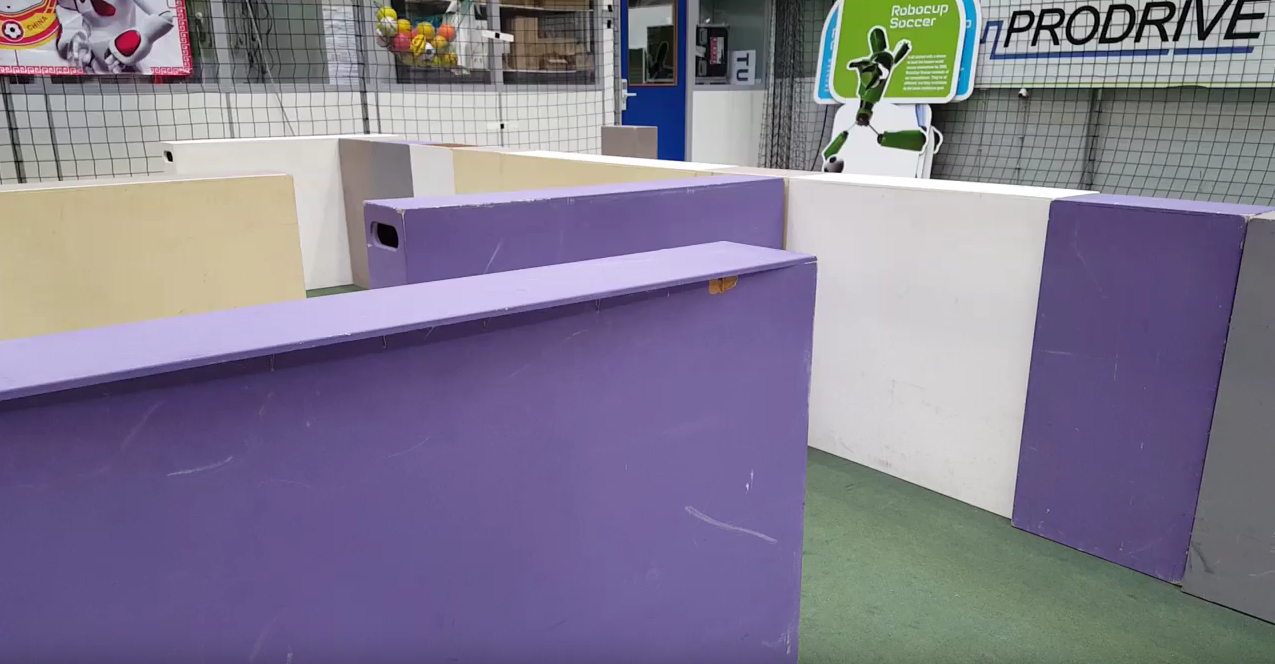 |
a picture of our desk after a hard and sleepless "emc" night
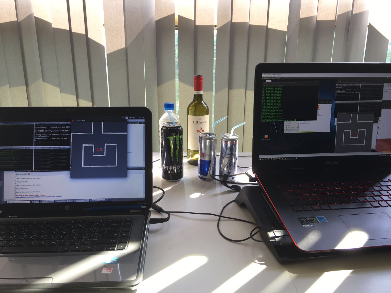
and below a picture of our group with our tutor Yanick and PICO, just after the maze competition.
