Embedded Motion Control 2012 Group 6: Difference between revisions
| (91 intermediate revisions by 5 users not shown) | |||
| Line 15: | Line 15: | ||
** Devision of work for the various blocks of functionality | ** Devision of work for the various blocks of functionality | ||
** First rough implementation: the robot is able to autonomously drive through the maze without hitting the walls | ** First rough implementation: the robot is able to autonomously drive through the maze without hitting the walls | ||
** | ** Progress on YouTube: [[File:week3.png|none|200px|link=http://youtu.be/qZ7NUgJI8uw?hd=1]] | ||
** The [http://cstwiki.wtb.tue.nl/images/CH08_group06_Other_Kernel_Objects.zip '''Presentation'''] is available online now. | ** The [http://cstwiki.wtb.tue.nl/images/CH08_group06_Other_Kernel_Objects.zip '''Presentation'''] is available online now. | ||
| Line 26: | Line 26: | ||
* '''Week 5''' | * '''Week 5''' | ||
** | ** Progress on YouTube: [[File:week5.png|none|200px|link=http://youtu.be/p8DRld3NVaY?hd=1]] | ||
* '''Week 6''' | * '''Week 6''' | ||
** | ** Perormed fantasticly during the CorridorChallenge | ||
** Progress on YouTube: [[File:week6.png|none|200px|link=http://youtu.be/hWepaa2UPkg?hd=1]] | |||
** Discussed and created a software architecture | |||
* '''Week 7''' | |||
** Progress on YouTube: [[File:week7.png|none|200px|link=http://youtu.be/2SzBqLgB6DU?hd=1]] | |||
* '''Week 8''' | |||
** Final presentation of group 6 as [http://cstwiki.wtb.tue.nl/images/Final_presentation_group06.zip '''presented''']. | |||
** Progress on YouTube: [[File:Final_contest_sim.png|none|200px|link=http://youtu.be/wZ1Io08ZNUg?hd=1]] | |||
This progress report aims to give an overview of the results of group 6. The software as developed has one specific goal: driving out of the maze. The robot first should drive into the maze. Hitting the wall results in a time penalty, which yields to the constraint not to hit the wall. In addition, speed is also of importance to set an unbeatable time. | |||
For the above addressed goal and constraints, requirements for the robot can be described. Movement is necessary to even start the competition, secondly vision (object detection) is mandatory to understand what is going on in the surroundings. But, the most important of course is strategy. Besides following the indicating arrows, a back-up strategy will be implemented. | |||
Different nodes will be developed, which form the building blocks of the complete software framework. | |||
== | ==Software Architecture== | ||
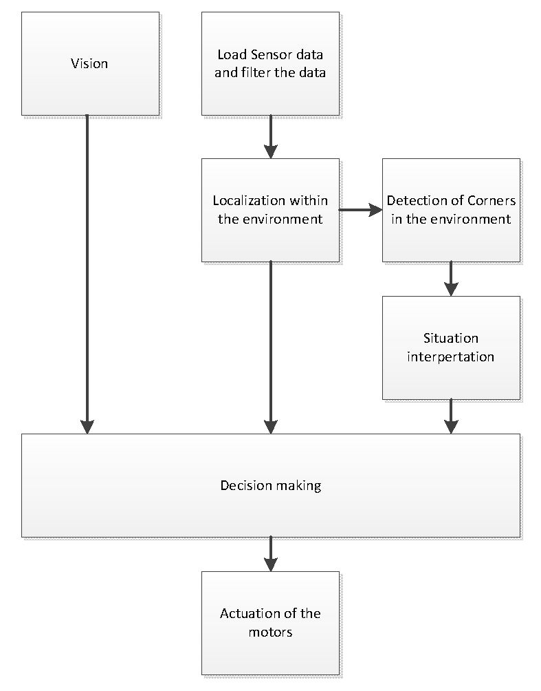
The architecture of our software can be seen in the Figure below. | |||
[[File:Architecture.png|none|1000px|''Architecture'']] | |||
it consists of three nodes nameley arrowNode, lineNode and controlNode. The lineNode will process the data gathered from the laser scanner and it will calculate lines which represent the walls based on that data. These lines will be published onto the lineData topic. Furthermore the lineNode will check certain properties of the detected walls which are published onto the wallStatus topic. For debugging purposes in the simulator a visualization_marker topic is published | |||
Besides the lineData and wallStatus, the controlNode is subscribed to the robot_out topic which contains the odometry data. The controlNode contains the navigation algorithm which controls the robot and sends the twistMessages on the robot_in topic. The algorithm within the controlNode is divided into separate states. It has been chosen, not to divide these separate states into different nodes, in order to reduce the communication overhead. Since the states within the controlNode do not need to be executed parallel, there is no need for separate nodes. | |||
When the robot is heading for a T-junction, the controlNode can call the arrowService, a member of the arrowNode, by sending requesting the service via pollArrow. This has been implemented as a service, in order to reduce the amount of bandwidth used during regular operation (i.e. non polling). | |||
==Arrow Detection (arrowNode)== | |||
The arrows help the robot navigating through the maze. In order to decide where to go, the robot should be able to process the following steps: | The arrows help the robot navigating through the maze. In order to decide where to go, the robot should be able to process the following steps: | ||
* | * Check for red objects | ||
* | * Identify an arrow shape if red objects are found on the wall | ||
* Determine the arrow point direction if arrow shape has been found | |||
* | * Use the obtained information to guide the robot | ||
===Brainstorm=== | ===Brainstorm=== | ||
| Line 71: | Line 72: | ||
With these observations in mind, clearly, a different approach is necessary. Different literature is studied to find the best practice. It turned out that image recognition does not cover the objective correctly (see for example<ref>[http://www.springerlink.com/content/qk2544412r717375/fulltext.pdf Noij2009239 on Springer.]</ref> ), it is better to use the term ''pattern recognition''. Using this term in combination with Linux one is directed to various sites mentioning OpenCV<ref>http://www.shervinemami.co.cc/blobs.html</ref><ref>http://opencv.willowgarage.com/documentation/cpp/index.html</ref> , which is also incorporated in ROS<ref>http://www.ros.org/wiki/vision_opencv</ref><ref>http://pharos.ece.utexas.edu/wiki/index.php/How_to_Use_a_Webcam_in_ROS_with_the_usb_cam_Package</ref>. In addition different books discus OpenCV | With these observations in mind, clearly, a different approach is necessary. Different literature is studied to find the best practice. It turned out that image recognition does not cover the objective correctly (see for example<ref>[http://www.springerlink.com/content/qk2544412r717375/fulltext.pdf Noij2009239 on Springer.]</ref> ), it is better to use the term ''pattern recognition''. Using this term in combination with Linux one is directed to various sites mentioning OpenCV<ref>http://www.shervinemami.co.cc/blobs.html</ref><ref>http://opencv.willowgarage.com/documentation/cpp/index.html</ref> , which is also incorporated in ROS<ref>http://www.ros.org/wiki/vision_opencv</ref><ref>http://pharos.ece.utexas.edu/wiki/index.php/How_to_Use_a_Webcam_in_ROS_with_the_usb_cam_Package</ref>. In addition different books discus OpenCV | ||
Open Source Computer Vision Library - Reference Manual by Intel | Open Source Computer Vision Library - Reference Manual by Intel | ||
Learning openCV by O'Reilly | Learning openCV by O'Reilly Besides robustness, it is learned that the following possible problems should be taken into account namely different light source and colours close to red. | ||
===Algorithm=== | ===Algorithm=== | ||
| Line 80: | Line 81: | ||
# Find contours using Canny algorithm | # Find contours using Canny algorithm | ||
# Approximate the found polygons | # Approximate the found polygons | ||
# Detect the biggest arrow using characteristic arrow properties ( | # Detect the biggest arrow using characteristic arrow properties (number of corners, concavity) | ||
#; If an arrow is found | #; If an arrow is found | ||
## Determine arrow bounding box | ## Determine arrow bounding box | ||
| Line 90: | Line 91: | ||
#; Report no result | #; Report no result | ||
=== | ===Discussion=== | ||
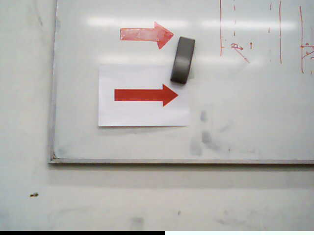
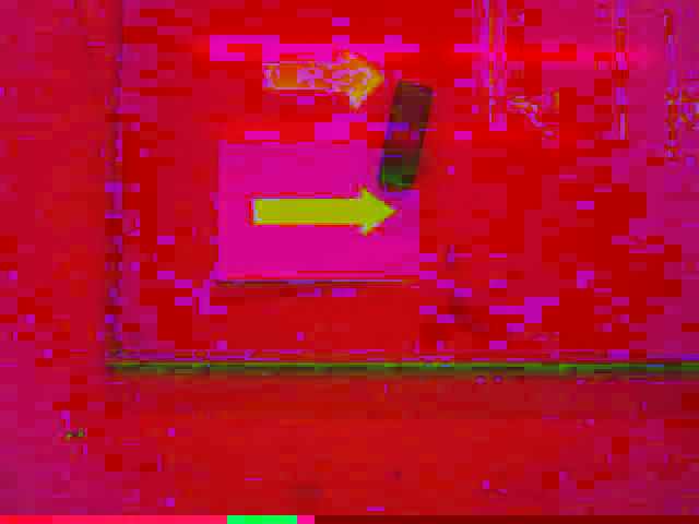
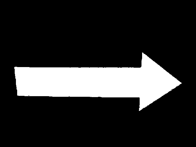
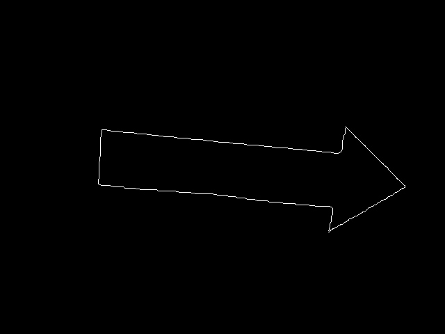
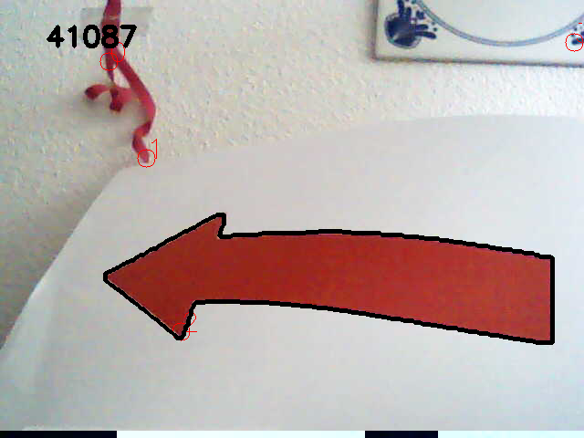
The pictures below show the first steps from the algorithm, were an arrow is correctly detected. | The pictures below show the first steps from the algorithm, were an arrow is correctly detected. | ||
| Line 105: | Line 106: | ||
Before continuing the algorithm, some remarks on possible flaws are made. | Before continuing the algorithm, some remarks on possible flaws are made. | ||
The picture below, however not so clearly, indicates the light source problem. The HSV transform is not homogeneous for the arrow, due the white stripe in the original file. This resulted in a very noise canny detection and other issues in the rest of the algorithm. | The picture below, however not so clearly, indicates the light source problem. The HSV transform is not homogeneous for the arrow, due the white stripe in the original file. This resulted in a very noise canny detection and other issues in the rest of the algorithm. | ||
| Line 123: | Line 119: | ||
Clearly, the algorithm is fooled. False corners are detected on both objects. Light influences the way red is detected, as a result setting the boundary's for the HSV extraction is quite tricky and dependent on the actual light environment. | Clearly, the algorithm is fooled. False corners are detected on both objects. Light influences the way red is detected, as a result setting the boundary's for the HSV extraction is quite tricky and dependent on the actual light environment. | ||
=== | ===CAPA=== | ||
As mentioned previously, problems with the HSV extraction were expected. During testing, it turned out the detection on the Pico camera differed from the used USB webcam used for the results in the above discussion. Besides possible different colour schemes, lenses and codecs, the different resolution yielded the biggest concerns. Optimal control of the HSV parameter setting was necessary, as less pixels where available for detecting purposes (i.e. requiring a more robust algorithm). | |||
With the published rosbag file by the tutors, this problem was studied in more detail. Apparently, the yellow door and red chair are challenging objects for proper filtering. As changing variables, making the code and testing the result got boring, some proper Computer Aided Parameter Adjustment (CAPA) was developed. See the result in the figure below. | |||
{| class="fig_table" | {| class="fig_table" | ||
| [[File: | | [[File:arrow_calibration.png|thumb|none|275px|''Proper calibration made possible with CAPA'']] | ||
|} | |} | ||
In | In the code it is possible to set a single define (#define CALIBRATION) in order to let the algorithm run in calibration mode. In this mode the algorithm will not run as a service, but it will continuously process the video stream. Doing this, the program will output the results of the separate steps of the algorithm to the screen. Together with this a set of sliders are displayed, with which the user can adjust the parameters of the algorithm in real-time (i.e. the result of the parameter is directly visible). CAPA facilitated a very easy and robust calibration method. Besides for different light situations, we could have cooped with blue instead of red arrows. Using CAPA, parameter adjustment is much faster as the constant rebuilding of the code is unnecessary. During the last test moment, different rosbags were created, Pico placed 0.5, 1 and 1.5 meter from a wall with the arrow pointing in both directions (six different rosbags). Using CAPA, we could for 0.5 and 1.0 meter in all cases (i.e. 100% good detection, no false information) and for each direction detect the direction. | ||
The effect of CAPA is clearly shown in the following movie: | |||
[[File:CAPA.png|none|200px|link=http://youtu.be/zxXUmH04n_c?hd=1]] | |||
=== | ===Service=== | ||
Using the ROS services environment, the limitation of bandwidth was possible. It turned out that processing the images is time consuming and costs CPU time. As the camera refreshes with roughly 1.5Hz, a service was made. Upon arriving, Pico stands still for roughly 3 seconds and identifies for four successive images the arrowdirection. Al tough 100% positive results were obtained during testing, the algorithm is build such that only a majority of one single direction is communicated. If two times left and two time right is the result, the service would return NONE, i.e. no arrow detected. | |||
==lineNode== | |||
The lineNode is responsible for a number of tasks related to detected lines (walls) in the environment of the robot. | |||
* Line detection | |||
* | * Dead path detection | ||
* | * Free path detection | ||
* Path width detection | |||
* T-junction detection | |||
===Line detection=== | |||
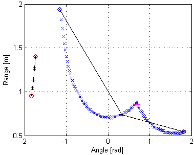
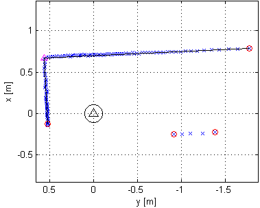
Since both the corridor and maze challenge do only contain straight walls, without other disturbing objects, the strategy is based upon information about walls in the neighborhood of the robot. These can be walls near the actual position of the robot, but also a history of waypoints derived from the wall-information. The wall-information is extracted from the lasersensor data. The detection algorithm needs to be robust, since sensor data will be contaminated by noise and the actual walls will not be perfectly straight lines and may be non-ideally aligned. | Since both the corridor and maze challenge do only contain straight walls, without other disturbing objects, the strategy is based upon information about walls in the neighborhood of the robot. These can be walls near the actual position of the robot, but also a history of waypoints derived from the wall-information. The wall-information is extracted from the lasersensor data. The detection algorithm needs to be robust, since sensor data will be contaminated by noise and the actual walls will not be perfectly straight lines and may be non-ideally aligned. | ||
An arrival of lasersensor data (configured at 5Hz) is followed by a call to the wall detection algorithm, which returns an array of line objects. These line objects contain the mathematical description of the surrounding walls and are used by the strategy algorithm. The same lines are also published as markers for visualization and debugging in RViz. | |||
The wall detection algorithm consists of the following steps: | The wall detection algorithm consists of the following steps: | ||
* Set measurements outside the range of interest to a large value, to exclude them from being detected as a wall. | * Set measurements outside the range of interest to a large value, to exclude them from being detected as a wall. | ||
* Apply a simple filter, to eliminate laserpoints with large measurement error. | |||
* Using the first and second derivative of the measurement points, the sharp corners and end of walls are detected. This gives a first rough list of lines. | * Using the first and second derivative of the measurement points, the sharp corners and end of walls are detected. This gives a first rough list of lines. | ||
* A line being detected may still contain one or multiple corners. Two additional checks are done recursively at each detected line segment. | * A line being detected may still contain one or multiple corners. Two additional checks are done recursively at each detected line segment. | ||
** The line is split in half. The midpoint is connected to both endpoints. For each measurement point | ** The line is split in half. The midpoint is connected to both endpoints. For each measurement point at a certain angle (in the polar-grid), the corresponding point on the linear line is calculated. This calculated point is then subtracted from the measured distance. This results in the difference between the measured and linear line. For both the first and second linear line, the maximum difference is searched. If this difference is above a calibrated threshold value, a embedded corner is found and the original line is split into two segments. | ||
** In certain unfavorable conditions a detected line may still contain a corner. The endpoints of the | ** In certain unfavorable conditions a detected line may still contain a corner. The endpoints of the known lines are connected (in the xy-grid) and the minimum and maximum peaks of the difference between measured and linear lines are observed to find any remaining corners. Again, these peak values are compared to a calibrated threshold, to avoid splitting lines on measurement errors or objects that do not contain perfectly straight walls. | ||
* Lines that do not contain enough measurement points to be regarded as reliable are thrown away. | * Lines that do not contain enough measurement points, to be regarded as reliable, are thrown away. | ||
The figures shown below | The figures shown below give a rough indication of the steps involved and the result. | ||
{| class="fig_table" | {| class="fig_table" | ||
| [[File:Line_detection1.png|thumb| | | [[File:Line_detection1.png|thumb|yes|275px|''Lasersensor data, polar-grid'']] | ||
| [[File:Line_detection2.png|thumb|none|275px|''Lasersensor data, xy-grid'']] | | [[File:Line_detection2.png|thumb|none|275px|''Lasersensor data, xy-grid'']] | ||
|} | |} | ||
| Line 175: | Line 167: | ||
Characteristic properties of each line are saved. The typical equation of a straight line (y=c*x+b) can be used to virtually extend a wall to any desired position, since the coefficients are saved. Also, the slope of the line indicates the angle of the wall relative to the robot. Furthermore the endpoints are saved by their x- and y-coordinate and index inside the array of laser measurements. Some other parameters (range of interest, tolerances, etc) are introduced to match the algorithm to the simulator and real robot. Several experiments proved the algorithm to function properly. This is an important step, since all higher level algorithms are fully dependent on the correctness of the provided line information. | Characteristic properties of each line are saved. The typical equation of a straight line (y=c*x+b) can be used to virtually extend a wall to any desired position, since the coefficients are saved. Also, the slope of the line indicates the angle of the wall relative to the robot. Furthermore the endpoints are saved by their x- and y-coordinate and index inside the array of laser measurements. Some other parameters (range of interest, tolerances, etc) are introduced to match the algorithm to the simulator and real robot. Several experiments proved the algorithm to function properly. This is an important step, since all higher level algorithms are fully dependent on the correctness of the provided line information. | ||
===Dead path detection=== | |||
The lineNode also provides an improvement of the maze-solving speed by detecting the dead-ends at the left and right side of the robot.This is done by comparing two laserpoints next to each other to a configured threshold value. When a jump in the laser scanner data is detected, there shouldn't be a dead end. There is also a second check to prevent walking into a dead end by detecting a bad connection between two walls. | |||
== | ===Free path detection=== | ||
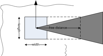
When arriving at a waypoint, the controlNode has to make a decision which path to take next. One of the variables being used is a set of booleans which describe whether the front, left and right side of the robot is not occupied by laserpoints and, therefore, free to drive. The procedure is as follows: The width and length of the robot is known. Furthermore, a parameter is specified at which distance (free_distance) from the robot should be checked for a free path. Combining these distances, a range of laserpoints can be selected to further investigate. These laserpoints are compared to the distance that the points should minimally have (free_distance). If one of the points is smaller than this distance, the path is blocked. This procedure is performed for front, left and right side of the robot. | |||
{| class="fig_table" | |||
| [[File:Path_free.png|thumb|none|275px|''Free distance'']] | |||
|} | |||
===Path width detection=== | |||
To adapt the navigation to a changing environment, the path widths that the robot encounters are detected. When driving in a path with a wall at the left and right side, the front path width is easily detected by a summation of the distance to the left and right wall. The left path width is detected when a wall appears up front and the wall at the left side does not continue up to the wall in front. The path width is calculated by taking the distance between the endpoint of the left wall to a point at the wall in front, whereby the calculated distance is perpendicular to the wall in front. The same procedure is applied for detecting the right path width. The implementation could be made quite easily, since all necessary data is already available from the lineNode. | |||
==Project standards== | {| class="fig_table" | ||
| [[File:Path_width.png|thumb|none|500px|''Path widths as defined.'']] | |||
|} | |||
===T-junction detection=== | |||
When arriving at a T-junction, the camera will be used to look for an arrow indication at the wall in front. This is the only situation that an arrow indication is expected, so only this type of waypoint should be detected. The procedure is fairly simple. When driving between a left and right wall a wall might pop up at the front (might also be at the left or right side, but front refers to a line perpendicular to the driving direction). A check is then done to check whether the left and right wall are continueing up to the front wall, or if there are sidepaths. If this is the case for both the left and right side, a T-junction is detected. When approaching the T-junction at a short distance, the left and right walls are not in sight of the lasersensor any more and an automatic switch to another approach is done. The T-junction detection is now only a check whether the left and right path are free and the front path is not free (see free path detection). This second approach may only be used when preceded by a detected T-junction with the first approach. An additional condition added for robustness is that the wall in front of the robot should be within 80-100 degrees angle with forwards direction of the robot. | |||
[[File:Tjunction.png]] | |||
===Node operation=== | |||
As described in the software architecture section, the lineNode has the laserdata topic as input. The output of the lineNode is a topic lineData, wallStatus and visualization_marker. The basic operation of the node is shown by the steps below. | |||
* Initialize ROS node structure | |||
* Create local callback queue for this node | |||
* Set looprate at 5 Hz | |||
* Subscribe to /robot/body/laser topic with bufferlength 1 to receive only the latest measurement | |||
* Register publishers for /lineData, /wallStatus and /visualization_marker topics | |||
* Enter main loop | |||
** Reset lines and status variables | |||
** Allow waiting laserdata callback to happen | |||
** Process lines | |||
** Publish /lineData | |||
** Update dead ends | |||
** Update free paths | |||
** Update path widths | |||
** Update T-junction | |||
** Publish /wallStatus | |||
** Publish /visualization_marker for line visualization in RViz (at 1Hz) | |||
** Update parameters received from rosparam (only active during calibration) | |||
** Cycle at 5Hz | |||
The definition of the /lineData messagetype: | |||
<pre>uint16 size | |||
uint16[] headIdx | |||
uint16[] tailIdx | |||
float32[] headX | |||
float32[] headY | |||
float32[] tailX | |||
float32[] tailY | |||
float32[] angleRad | |||
float32[] angleDeg | |||
float32[] b | |||
float32[] c | |||
float32[] dstMin | |||
uint8[] wall</pre> | |||
The definition of the /wallStatus messagetype: | |||
<pre>bool frontFree | |||
bool leftFree | |||
bool rightFree | |||
float32 frontWidth | |||
float32 leftWidth | |||
float32 rightWidth | |||
bool deadPath | |||
bool wallTooClose | |||
bool leftDeadEnd | |||
bool rightDeadEnd | |||
bool TJunction</pre> | |||
Watch the video below to see some results of the lineNode. | |||
[[File:week7.png|none|200px|link=http://youtu.be/2SzBqLgB6DU?hd=1]] | |||
==Navigation algorithm (controlNode)== | |||
The navigation algorithm is implemented in the controlNode and uses odometry data, line data (from the lineNode) and arrow data (from the arrowNode) to control Pico. The lineNode provides the following information: | |||
* A set of lines, extracted from the laserscan data. | |||
** For each line, properties such as angle with respect to Pico, shortest distance to Pico and a mathematical description of the line (<math>y = ax + b</math>). | |||
** Since a mathematical description of each line is provided, the length of each line can be virtually extended to infinite lengths. This enables the algorithm to stop Pico at the center of an adjacent corridor. | |||
* A pointer to three special lines: the line right next to Pico, the line in front and the line left next to Pico. | |||
* The width of the corridor on the right of Pico, in front of Pico and on the left of Pico (if any). | |||
* Information about whether the corridors to the right, in front and to the left are free or blocked. | |||
* Information about whether these corridors have a dead and or not. | |||
* Information about whether Pico is currently on a T-junction or not. | |||
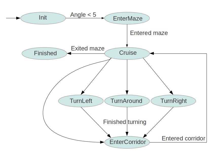
To be able to manage the complexity of the controlNode, the controlNode is designed as a statemachine consisting of the following states: | |||
* '''Init:''' This is the initial state. It uses the line data to align Pico with the entrance of the maze to prevent collisions while entering it. | |||
* '''EnterMaze:''' In this state, Pico will enter the maze while driving parallel to the walls. | |||
* '''Cruise:''' This is the main state, it keeps Pico in the middle of the corridor while driving parallel to the walls to the end of the corridor. At the end of the corridor it decides where to go next. | |||
* '''TurnRight:''' In this state, Pico will make a 90 degree turn to the right. | |||
* '''TurnLeft:''' In this state, Pico will make a 90 degree turn to the left. | |||
* '''TurnAround:''' In this state, Pico will make a 180 degree turn. | |||
* '''EnterCorridor:''' This state is an intermediate state between turning and cruising. After a turn is made, the corridor needs to be entered before the cruise mode can be enabled again. | |||
* '''Finished:''' In this state, Pico is outside of the maze and therefore finished the competition. | |||
[[File:StateMachine.jpg]] | |||
===Cruise mode=== | |||
The state machine can be found in the above diagram. The cruise mode is the most important one. It uses the distance to the wall right and left of Pico to keep the middle of the corridor. Furthermore, it uses the angles with respect to the right and left wall to drive parallel with the walls. Corrections are made using a simple, but effective p-controller. | |||
If a wall in front of Pico is detected, the algorithm makes the decision of what the new direction should be. After it made a decision, it stores the width of corresponding corridor (say <math>w</math>). Now it can drive forward until the distance of the wall in front is <math>\frac{w}{2}</math>. Using this approach Pico will always remain in the middle of the corridor. | |||
The algorithm will make decisions using the following scheme: | |||
* If Pico is at a T-junction. The arrowNode will be requested to check for an arrow. If an arrow is detected, Pico will turn in the resulting direction. | |||
* If Pico is not at a T-junction, or no arrow is detected it will check whether the corridor to the right/front/left is free and is not a dead end (another order of checking the corridors can be selected by 'define' statements). | |||
* If none of the corridors is free, the algorithm will decide to turn around. | |||
If the algorithm decides to make a turn, the controlNode will store the current angle (from odometry data, say 'startAngle') and go to the corresponding state (turnRight/turnLeft/turnAround). In case the algorithm decides to go straight on, no turning is needed and therefore the algorithm will jump directly to the EnterCorridor state. | |||
In case the algorithm detects that Pico has exited the maze (using the line information), the controlNode will go the the finished state and Pico will be stopped. | |||
===Turn modes=== | |||
Three turn modes are implemented in the controlNode: turnRight/turnLeft/turnAround. These states use the odometry data to calculate the current angle and checks the difference with the start angle stored just before entering this state. This difference is fed to a p-controller to turn Pico to the desired angle. | |||
Since the orientation of Pico is stored in the odometry data as a quaternion, a conversion is required to extract roll, pitch and yaw angles. The following equations can be found on [http://en.wikipedia.org/wiki/Conversion_between_quaternions_and_Euler_angles#Conversion Convert_quaternions] | |||
:<math>\begin{bmatrix} | |||
\phi \\ \theta \\ \psi | |||
\end{bmatrix} = | |||
\begin{bmatrix} | |||
\mbox{atan2} (2(q_0 q_1 + q_2 q_3),1 - 2(q_1^2 + q_2^2)) \\ | |||
\mbox{arcsin} (2(q_0 q_2 - q_3 q_1)) \\ | |||
\mbox{atan2} (2(q_0 q_3 + q_1 q_2),1 - 2(q_2^2 + q_3^2)) | |||
\end{bmatrix} </math> | |||
Where: | |||
* Roll – <math>\phi</math>: rotation about the X-axis | |||
* Pitch – <math>\theta</math>: rotation about the Y-axis | |||
* Yaw – <math>\psi</math>: rotation about the Z-axis | |||
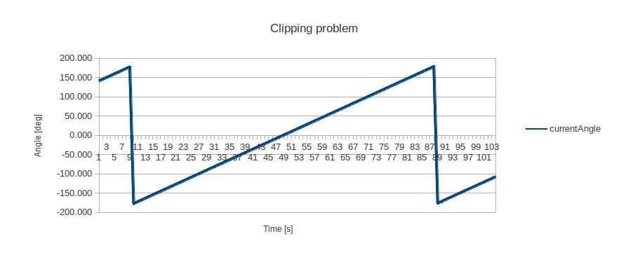
These equations are implemented and tested. The graph below shows the results of one of these tests. In this case, Pico turns with a constant velocity around its axis. It can be seen that the value of currentAngle increases linearly until the value reaches 180 degrees. At this point the value clips to -180 degrees. This clipping effect causes problems when calculating the difference between the current angle and the angle before turning. | |||
[[File:AngleData.jpg]] | |||
This problem is solved by keeping track of the difference of two consecutive angle values. If the difference is bigger than 180 degrees (i.e. a 'clip' has occurred), the calculation of the difference between start and current angle is corrected. Using this correction together with the p-controller, the navigation algorithm is able to make nice 90 and 180 degree turns. After Pico successfully made its turn it first needs to enter the corridor in front before the normal cruise mode can be enabled again. Therefore, the controlNode will go to state EnterCorridor after turning has finished. | |||
===Enter corridor mode=== | |||
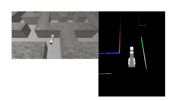
After the algorithm just reached the Enter corridor state, there is a free corridor in front of Pico, but the lineNode has detected a wall in front of Pico. In this case (because the corridor in front of Pico is free) the part of the line right in front of Pico is virtual. | |||
{| class="fig_table" | |||
| [[File:EnterCorridor.jpg|thumb|none|475px|''Viritual line for enter mode (the detected wall in front of Pico is marked blue).']] | |||
|} | |||
Using the Enter corridor mode, the algorithm will enter the corridor in front of Pico and thereby crossing the virtual wall in front. In this mode, the algorithm will also make sure that Pico remains in the middle of the corridor and aligns Pico with the wall left and right. After Pico has crossed the virtual line in front, the algorithm will jump back to the cruise mode. | |||
This navigation algorithm is tested thoroughly in different mazes. In all cases it succeeded to navigate through the maze without hitting the walls. | |||
This can be seen in the following movie: | |||
[[File:week7.png|none|200px|link=http://youtu.be/2SzBqLgB6DU?hd=1]] | |||
==Way of Testing== | |||
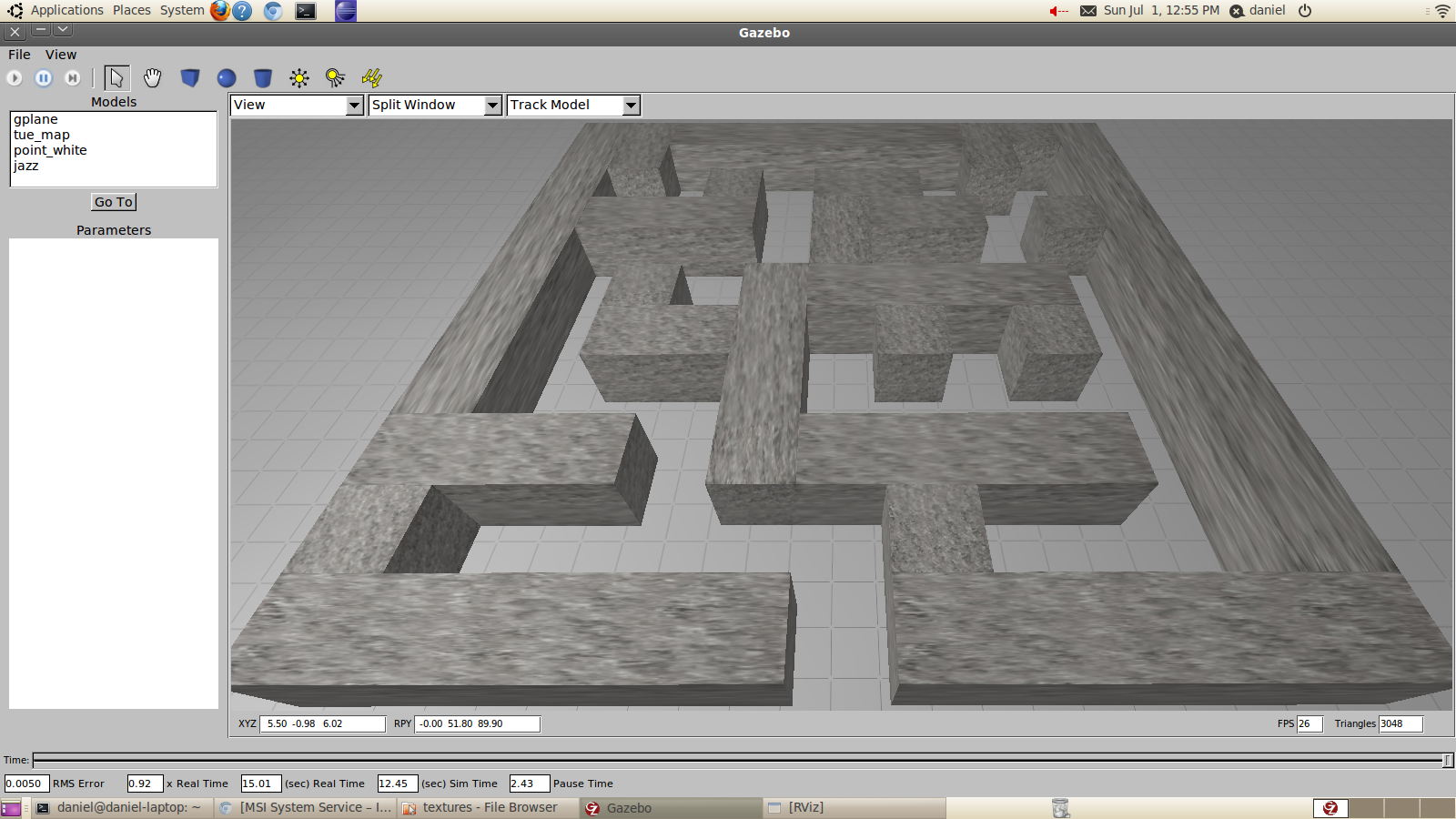
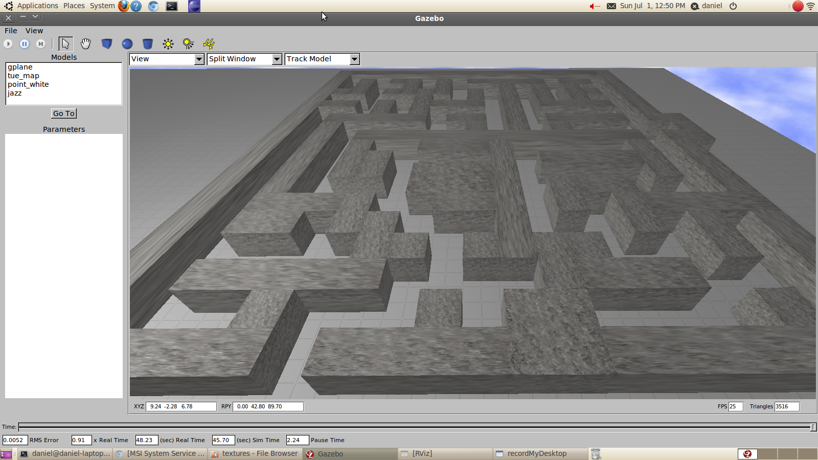
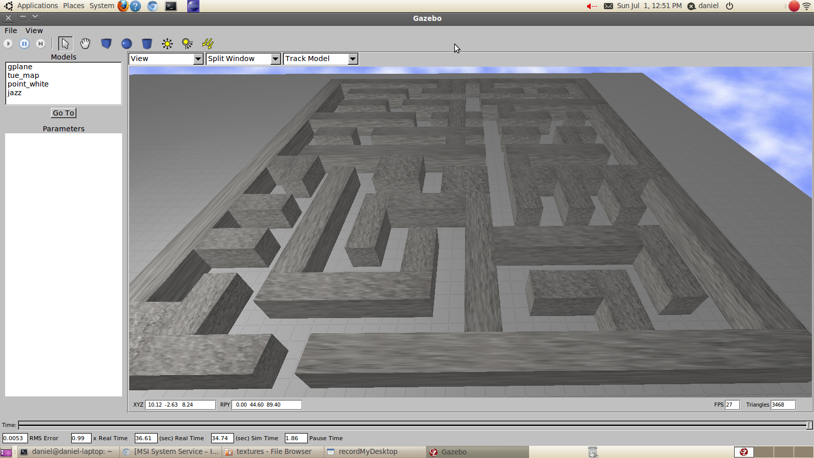
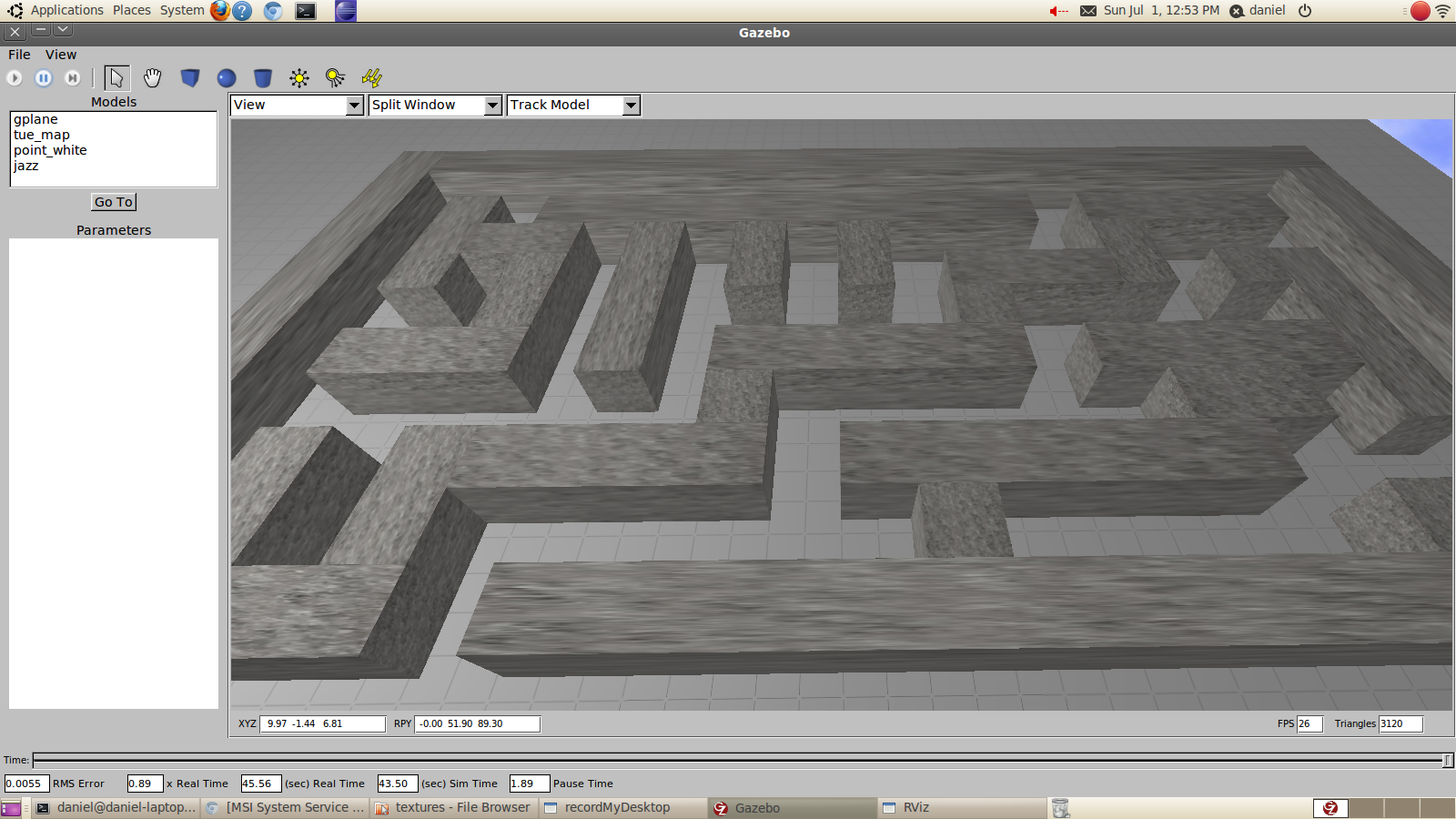
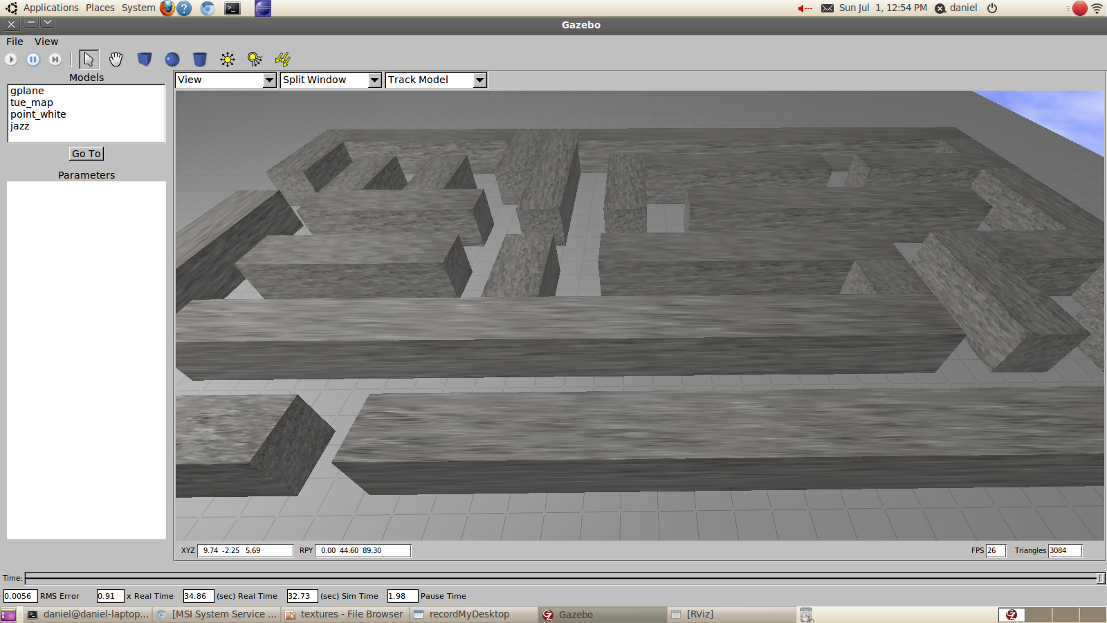
Fortounatly we are able to use a simulator. This helps a lot and was a good way to solve a lot of problems and avoids wasting our limited testing time on the real robot. | |||
A few mazes has been created during the course, they are also mirrored to create also new situations. | |||
{| class="fig_table" | |||
| [[File:Mazes6.png|thumb|none|200px|''Lasersensor data, Original maze'']] | |||
| [[File:Mazes2.png|thumb|none|200px|''Lasersensor data, Big maze with a lot of different situations'']] | |||
| [[File:Mazes3.png|thumb|none|200px|''Lasersensor data, Big maze with improved different situations'']] | |||
| [[File:Mazes4.png|thumb|none|200px|''Lasersensor data, Small maze with returning situations to test a specific problem'']] | |||
| [[File:Mazes5.png|thumb|none|200px|''Lasersensor data, Testing with floating walls'']] | |||
|} | |||
The most hard to solve problems occur by winding paths. This problems are solved by using limited ranges and giving priorities to line data or laser data points. | |||
==Project agreements== | |||
===Coding standards=== | |||
* Names are given using camelCase standard | |||
* Parameters are placed in header files by use of defines | |||
* For indents TAB characters are used | |||
* An opening { follows right behind an if, while, etc... statement and not on the next line | |||
* Else follows directly after an closing } | |||
* Comment the statement that is being closed after a closing } | |||
===SVN guidelines=== | ===SVN guidelines=== | ||
| Line 199: | Line 349: | ||
*# use version B | *# use version B | ||
*# show the differences | *# show the differences | ||
===Add laser frame to rviz=== | |||
<pre>rosrun tf static_transform_publisher 0 0 0 0 0 0 /base_link /laser 10</pre> | |||
===TAB problems in Kate editor=== | ===TAB problems in Kate editor=== | ||
In Kate, TAB inserts spaces instead of true tabs. According to <ref>[https://bugs.launchpad.net/ubuntu/+source/kdesdk/+bug/282234]</ref> you should set '''tab width''' equal '''indention width'''. Open Settings -> Configure Kate, in the editing section you can set tab width (e.g. 8). Another section is found for Indention, set indention width to the same value. | In Kate, TAB inserts spaces instead of true tabs. According to<ref>[https://bugs.launchpad.net/ubuntu/+source/kdesdk/+bug/282234]</ref> you should set '''tab width''' equal '''indention width'''. Open Settings -> Configure Kate, in the editing section you can set tab width (e.g. 8). Another section is found for Indention, set indention width to the same value. | ||
===How to create a screen video?=== | ===How to create a screen video?=== | ||
| Line 224: | Line 379: | ||
<ref>[http://www.ros.org/reps/rep-0103.html#axis-orientation Standard Units of Measure and Coordinate Conventions.]</ref> | <ref>[http://www.ros.org/reps/rep-0103.html#axis-orientation Standard Units of Measure and Coordinate Conventions.]</ref> | ||
<ref>[http://www.robotshop.com/jazz-security-robot-2.html Specs of the robot (buy one!).]</ref> | <ref>[http://www.robotshop.com/jazz-security-robot-2.html Specs of the robot (buy one!).]</ref> | ||
<ref>[http://en.wikipedia.org/wiki/Conversion_between_quaternions_and_Euler_angles#Conversion Quaternion conversions]</ref> | |||
<references /> | <references /> | ||
Latest revision as of 23:09, 1 July 2012
Progress
Progress of the group. The newest item is listed on top.
- Week 1
- Started with tutorials (all)
- Installed ROS + Eclipse (all)
- Installed Ubuntu (all)
- Week 2
- Finished with tutorials (all)
- Practiced with simulator (all)
- Investigated sensor data(all)
- Week 3
- Overall design of the robot control software
- Devision of work for the various blocks of functionality
- First rough implementation: the robot is able to autonomously drive through the maze without hitting the walls
- Progress on YouTube:
- The Presentation is available online now.
- Week 4
- Studying chapter 8
- Creating presentation slides (finished)
- Rehearsing presentation over and over again (finished)
- Creating dead end detection (finished)
- Creating pre safe system (finished)
- Week 6
- Week 8
- Final presentation of group 6 as presented.
- Progress on YouTube:
This progress report aims to give an overview of the results of group 6. The software as developed has one specific goal: driving out of the maze. The robot first should drive into the maze. Hitting the wall results in a time penalty, which yields to the constraint not to hit the wall. In addition, speed is also of importance to set an unbeatable time.
For the above addressed goal and constraints, requirements for the robot can be described. Movement is necessary to even start the competition, secondly vision (object detection) is mandatory to understand what is going on in the surroundings. But, the most important of course is strategy. Besides following the indicating arrows, a back-up strategy will be implemented.
Different nodes will be developed, which form the building blocks of the complete software framework.
Software Architecture
The architecture of our software can be seen in the Figure below.
it consists of three nodes nameley arrowNode, lineNode and controlNode. The lineNode will process the data gathered from the laser scanner and it will calculate lines which represent the walls based on that data. These lines will be published onto the lineData topic. Furthermore the lineNode will check certain properties of the detected walls which are published onto the wallStatus topic. For debugging purposes in the simulator a visualization_marker topic is published
Besides the lineData and wallStatus, the controlNode is subscribed to the robot_out topic which contains the odometry data. The controlNode contains the navigation algorithm which controls the robot and sends the twistMessages on the robot_in topic. The algorithm within the controlNode is divided into separate states. It has been chosen, not to divide these separate states into different nodes, in order to reduce the communication overhead. Since the states within the controlNode do not need to be executed parallel, there is no need for separate nodes.
When the robot is heading for a T-junction, the controlNode can call the arrowService, a member of the arrowNode, by sending requesting the service via pollArrow. This has been implemented as a service, in order to reduce the amount of bandwidth used during regular operation (i.e. non polling).
Arrow Detection (arrowNode)
The arrows help the robot navigating through the maze. In order to decide where to go, the robot should be able to process the following steps:
- Check for red objects
- Identify an arrow shape if red objects are found on the wall
- Determine the arrow point direction if arrow shape has been found
- Use the obtained information to guide the robot
Brainstorm
The ROS package provides a package for face detection[1]. One can see the image as a poor representation of a face, and teach the robot the possible appearances of this face. The program is thought to recognise a left pointing "face" and a right pointing "face". However, one can doubt the robustness of this system. First because the system is not intended for arrow recognition, i.e. it is misused. Possibly, some crucial elements for arrow recognition are not implemented in this package. Secondly, face recognition requires a frontal view check. If the robot and wall with the arrow are not perfectly in line, the package can possibly not identify the arrow. Thirdly, an arrow in a slight different orientation can not be detected.
With these observations in mind, clearly, a different approach is necessary. Different literature is studied to find the best practice. It turned out that image recognition does not cover the objective correctly (see for example[2] ), it is better to use the term pattern recognition. Using this term in combination with Linux one is directed to various sites mentioning OpenCV[3][4] , which is also incorporated in ROS[5][6]. In addition different books discus OpenCV Open Source Computer Vision Library - Reference Manual by Intel Learning openCV by O'Reilly Besides robustness, it is learned that the following possible problems should be taken into account namely different light source and colours close to red.
Algorithm
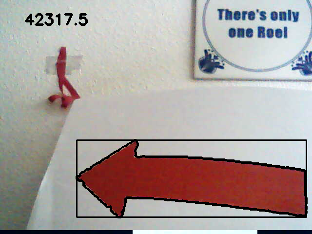
After studying the material discussed in the previous section, the following arrow detection algorithm is deduced:
- Open image
- Apply HSV transform
- Filter red colour from image
- Find contours using Canny algorithm
- Approximate the found polygons
- Detect the biggest arrow using characteristic arrow properties (number of corners, concavity)
- If an arrow is found
- Determine arrow bounding box
- Find corners on the bounding box
- Determine arrow orientation
- Report direction (i.e. left or right)
- Report no result
- If no arrow is found
- Report no result
Discussion
The pictures below show the first steps from the algorithm, were an arrow is correctly detected.
 |
 |
 |
 |
 |
 |
Before continuing the algorithm, some remarks on possible flaws are made.
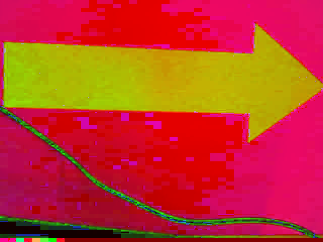
The picture below, however not so clearly, indicates the light source problem. The HSV transform is not homogeneous for the arrow, due the white stripe in the original file. This resulted in a very noise canny detection and other issues in the rest of the algorithm.
 |
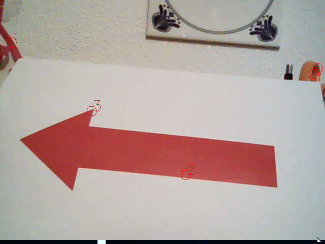
For sure, the arrow is printed on a white sheet of paper. Concerning the environment of the maze nothing is told, this forced us to check the robustness in an not so ideal environment. Colours close to red are, e.g. pink and orange. A test set-up was created consisting of orange scissors on one side and a nice pink ribbon on the other, see below.
 |
 |
Clearly, the algorithm is fooled. False corners are detected on both objects. Light influences the way red is detected, as a result setting the boundary's for the HSV extraction is quite tricky and dependent on the actual light environment.
CAPA
As mentioned previously, problems with the HSV extraction were expected. During testing, it turned out the detection on the Pico camera differed from the used USB webcam used for the results in the above discussion. Besides possible different colour schemes, lenses and codecs, the different resolution yielded the biggest concerns. Optimal control of the HSV parameter setting was necessary, as less pixels where available for detecting purposes (i.e. requiring a more robust algorithm). With the published rosbag file by the tutors, this problem was studied in more detail. Apparently, the yellow door and red chair are challenging objects for proper filtering. As changing variables, making the code and testing the result got boring, some proper Computer Aided Parameter Adjustment (CAPA) was developed. See the result in the figure below.
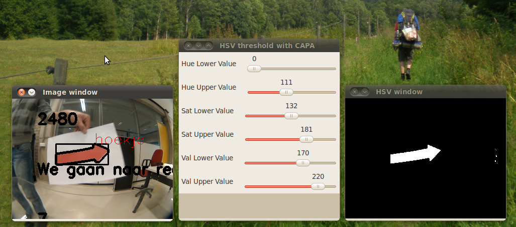 |
In the code it is possible to set a single define (#define CALIBRATION) in order to let the algorithm run in calibration mode. In this mode the algorithm will not run as a service, but it will continuously process the video stream. Doing this, the program will output the results of the separate steps of the algorithm to the screen. Together with this a set of sliders are displayed, with which the user can adjust the parameters of the algorithm in real-time (i.e. the result of the parameter is directly visible). CAPA facilitated a very easy and robust calibration method. Besides for different light situations, we could have cooped with blue instead of red arrows. Using CAPA, parameter adjustment is much faster as the constant rebuilding of the code is unnecessary. During the last test moment, different rosbags were created, Pico placed 0.5, 1 and 1.5 meter from a wall with the arrow pointing in both directions (six different rosbags). Using CAPA, we could for 0.5 and 1.0 meter in all cases (i.e. 100% good detection, no false information) and for each direction detect the direction.
The effect of CAPA is clearly shown in the following movie:
Service
Using the ROS services environment, the limitation of bandwidth was possible. It turned out that processing the images is time consuming and costs CPU time. As the camera refreshes with roughly 1.5Hz, a service was made. Upon arriving, Pico stands still for roughly 3 seconds and identifies for four successive images the arrowdirection. Al tough 100% positive results were obtained during testing, the algorithm is build such that only a majority of one single direction is communicated. If two times left and two time right is the result, the service would return NONE, i.e. no arrow detected.
lineNode
The lineNode is responsible for a number of tasks related to detected lines (walls) in the environment of the robot.
- Line detection
- Dead path detection
- Free path detection
- Path width detection
- T-junction detection
Line detection
Since both the corridor and maze challenge do only contain straight walls, without other disturbing objects, the strategy is based upon information about walls in the neighborhood of the robot. These can be walls near the actual position of the robot, but also a history of waypoints derived from the wall-information. The wall-information is extracted from the lasersensor data. The detection algorithm needs to be robust, since sensor data will be contaminated by noise and the actual walls will not be perfectly straight lines and may be non-ideally aligned.
An arrival of lasersensor data (configured at 5Hz) is followed by a call to the wall detection algorithm, which returns an array of line objects. These line objects contain the mathematical description of the surrounding walls and are used by the strategy algorithm. The same lines are also published as markers for visualization and debugging in RViz.
The wall detection algorithm consists of the following steps:
- Set measurements outside the range of interest to a large value, to exclude them from being detected as a wall.
- Apply a simple filter, to eliminate laserpoints with large measurement error.
- Using the first and second derivative of the measurement points, the sharp corners and end of walls are detected. This gives a first rough list of lines.
- A line being detected may still contain one or multiple corners. Two additional checks are done recursively at each detected line segment.
- The line is split in half. The midpoint is connected to both endpoints. For each measurement point at a certain angle (in the polar-grid), the corresponding point on the linear line is calculated. This calculated point is then subtracted from the measured distance. This results in the difference between the measured and linear line. For both the first and second linear line, the maximum difference is searched. If this difference is above a calibrated threshold value, a embedded corner is found and the original line is split into two segments.
- In certain unfavorable conditions a detected line may still contain a corner. The endpoints of the known lines are connected (in the xy-grid) and the minimum and maximum peaks of the difference between measured and linear lines are observed to find any remaining corners. Again, these peak values are compared to a calibrated threshold, to avoid splitting lines on measurement errors or objects that do not contain perfectly straight walls.
- Lines that do not contain enough measurement points, to be regarded as reliable, are thrown away.
The figures shown below give a rough indication of the steps involved and the result.
 |
 |
Characteristic properties of each line are saved. The typical equation of a straight line (y=c*x+b) can be used to virtually extend a wall to any desired position, since the coefficients are saved. Also, the slope of the line indicates the angle of the wall relative to the robot. Furthermore the endpoints are saved by their x- and y-coordinate and index inside the array of laser measurements. Some other parameters (range of interest, tolerances, etc) are introduced to match the algorithm to the simulator and real robot. Several experiments proved the algorithm to function properly. This is an important step, since all higher level algorithms are fully dependent on the correctness of the provided line information.
Dead path detection
The lineNode also provides an improvement of the maze-solving speed by detecting the dead-ends at the left and right side of the robot.This is done by comparing two laserpoints next to each other to a configured threshold value. When a jump in the laser scanner data is detected, there shouldn't be a dead end. There is also a second check to prevent walking into a dead end by detecting a bad connection between two walls.
Free path detection
When arriving at a waypoint, the controlNode has to make a decision which path to take next. One of the variables being used is a set of booleans which describe whether the front, left and right side of the robot is not occupied by laserpoints and, therefore, free to drive. The procedure is as follows: The width and length of the robot is known. Furthermore, a parameter is specified at which distance (free_distance) from the robot should be checked for a free path. Combining these distances, a range of laserpoints can be selected to further investigate. These laserpoints are compared to the distance that the points should minimally have (free_distance). If one of the points is smaller than this distance, the path is blocked. This procedure is performed for front, left and right side of the robot.
 |
Path width detection
To adapt the navigation to a changing environment, the path widths that the robot encounters are detected. When driving in a path with a wall at the left and right side, the front path width is easily detected by a summation of the distance to the left and right wall. The left path width is detected when a wall appears up front and the wall at the left side does not continue up to the wall in front. The path width is calculated by taking the distance between the endpoint of the left wall to a point at the wall in front, whereby the calculated distance is perpendicular to the wall in front. The same procedure is applied for detecting the right path width. The implementation could be made quite easily, since all necessary data is already available from the lineNode.
 |
T-junction detection
When arriving at a T-junction, the camera will be used to look for an arrow indication at the wall in front. This is the only situation that an arrow indication is expected, so only this type of waypoint should be detected. The procedure is fairly simple. When driving between a left and right wall a wall might pop up at the front (might also be at the left or right side, but front refers to a line perpendicular to the driving direction). A check is then done to check whether the left and right wall are continueing up to the front wall, or if there are sidepaths. If this is the case for both the left and right side, a T-junction is detected. When approaching the T-junction at a short distance, the left and right walls are not in sight of the lasersensor any more and an automatic switch to another approach is done. The T-junction detection is now only a check whether the left and right path are free and the front path is not free (see free path detection). This second approach may only be used when preceded by a detected T-junction with the first approach. An additional condition added for robustness is that the wall in front of the robot should be within 80-100 degrees angle with forwards direction of the robot.
Node operation
As described in the software architecture section, the lineNode has the laserdata topic as input. The output of the lineNode is a topic lineData, wallStatus and visualization_marker. The basic operation of the node is shown by the steps below.
- Initialize ROS node structure
- Create local callback queue for this node
- Set looprate at 5 Hz
- Subscribe to /robot/body/laser topic with bufferlength 1 to receive only the latest measurement
- Register publishers for /lineData, /wallStatus and /visualization_marker topics
- Enter main loop
- Reset lines and status variables
- Allow waiting laserdata callback to happen
- Process lines
- Publish /lineData
- Update dead ends
- Update free paths
- Update path widths
- Update T-junction
- Publish /wallStatus
- Publish /visualization_marker for line visualization in RViz (at 1Hz)
- Update parameters received from rosparam (only active during calibration)
- Cycle at 5Hz
The definition of the /lineData messagetype:
uint16 size
uint16[] headIdx
uint16[] tailIdx
float32[] headX
float32[] headY
float32[] tailX
float32[] tailY
float32[] angleRad
float32[] angleDeg
float32[] b
float32[] c
float32[] dstMin
uint8[] wall
The definition of the /wallStatus messagetype:
bool frontFree
bool leftFree
bool rightFree
float32 frontWidth
float32 leftWidth
float32 rightWidth
bool deadPath
bool wallTooClose
bool leftDeadEnd
bool rightDeadEnd
bool TJunction
Watch the video below to see some results of the lineNode.
The navigation algorithm is implemented in the controlNode and uses odometry data, line data (from the lineNode) and arrow data (from the arrowNode) to control Pico. The lineNode provides the following information:
- A set of lines, extracted from the laserscan data.
- For each line, properties such as angle with respect to Pico, shortest distance to Pico and a mathematical description of the line ([math]\displaystyle{ y = ax + b }[/math]).
- Since a mathematical description of each line is provided, the length of each line can be virtually extended to infinite lengths. This enables the algorithm to stop Pico at the center of an adjacent corridor.
- A pointer to three special lines: the line right next to Pico, the line in front and the line left next to Pico.
- The width of the corridor on the right of Pico, in front of Pico and on the left of Pico (if any).
- Information about whether the corridors to the right, in front and to the left are free or blocked.
- Information about whether these corridors have a dead and or not.
- Information about whether Pico is currently on a T-junction or not.
To be able to manage the complexity of the controlNode, the controlNode is designed as a statemachine consisting of the following states:
- Init: This is the initial state. It uses the line data to align Pico with the entrance of the maze to prevent collisions while entering it.
- EnterMaze: In this state, Pico will enter the maze while driving parallel to the walls.
- Cruise: This is the main state, it keeps Pico in the middle of the corridor while driving parallel to the walls to the end of the corridor. At the end of the corridor it decides where to go next.
- TurnRight: In this state, Pico will make a 90 degree turn to the right.
- TurnLeft: In this state, Pico will make a 90 degree turn to the left.
- TurnAround: In this state, Pico will make a 180 degree turn.
- EnterCorridor: This state is an intermediate state between turning and cruising. After a turn is made, the corridor needs to be entered before the cruise mode can be enabled again.
- Finished: In this state, Pico is outside of the maze and therefore finished the competition.
Cruise mode
The state machine can be found in the above diagram. The cruise mode is the most important one. It uses the distance to the wall right and left of Pico to keep the middle of the corridor. Furthermore, it uses the angles with respect to the right and left wall to drive parallel with the walls. Corrections are made using a simple, but effective p-controller.
If a wall in front of Pico is detected, the algorithm makes the decision of what the new direction should be. After it made a decision, it stores the width of corresponding corridor (say [math]\displaystyle{ w }[/math]). Now it can drive forward until the distance of the wall in front is [math]\displaystyle{ \frac{w}{2} }[/math]. Using this approach Pico will always remain in the middle of the corridor.
The algorithm will make decisions using the following scheme:
- If Pico is at a T-junction. The arrowNode will be requested to check for an arrow. If an arrow is detected, Pico will turn in the resulting direction.
- If Pico is not at a T-junction, or no arrow is detected it will check whether the corridor to the right/front/left is free and is not a dead end (another order of checking the corridors can be selected by 'define' statements).
- If none of the corridors is free, the algorithm will decide to turn around.
If the algorithm decides to make a turn, the controlNode will store the current angle (from odometry data, say 'startAngle') and go to the corresponding state (turnRight/turnLeft/turnAround). In case the algorithm decides to go straight on, no turning is needed and therefore the algorithm will jump directly to the EnterCorridor state.
In case the algorithm detects that Pico has exited the maze (using the line information), the controlNode will go the the finished state and Pico will be stopped.
Turn modes
Three turn modes are implemented in the controlNode: turnRight/turnLeft/turnAround. These states use the odometry data to calculate the current angle and checks the difference with the start angle stored just before entering this state. This difference is fed to a p-controller to turn Pico to the desired angle.
Since the orientation of Pico is stored in the odometry data as a quaternion, a conversion is required to extract roll, pitch and yaw angles. The following equations can be found on Convert_quaternions
- [math]\displaystyle{ \begin{bmatrix} \phi \\ \theta \\ \psi \end{bmatrix} = \begin{bmatrix} \mbox{atan2} (2(q_0 q_1 + q_2 q_3),1 - 2(q_1^2 + q_2^2)) \\ \mbox{arcsin} (2(q_0 q_2 - q_3 q_1)) \\ \mbox{atan2} (2(q_0 q_3 + q_1 q_2),1 - 2(q_2^2 + q_3^2)) \end{bmatrix} }[/math]
Where:
- Roll – [math]\displaystyle{ \phi }[/math]: rotation about the X-axis
- Pitch – [math]\displaystyle{ \theta }[/math]: rotation about the Y-axis
- Yaw – [math]\displaystyle{ \psi }[/math]: rotation about the Z-axis
These equations are implemented and tested. The graph below shows the results of one of these tests. In this case, Pico turns with a constant velocity around its axis. It can be seen that the value of currentAngle increases linearly until the value reaches 180 degrees. At this point the value clips to -180 degrees. This clipping effect causes problems when calculating the difference between the current angle and the angle before turning.
This problem is solved by keeping track of the difference of two consecutive angle values. If the difference is bigger than 180 degrees (i.e. a 'clip' has occurred), the calculation of the difference between start and current angle is corrected. Using this correction together with the p-controller, the navigation algorithm is able to make nice 90 and 180 degree turns. After Pico successfully made its turn it first needs to enter the corridor in front before the normal cruise mode can be enabled again. Therefore, the controlNode will go to state EnterCorridor after turning has finished.
Enter corridor mode
After the algorithm just reached the Enter corridor state, there is a free corridor in front of Pico, but the lineNode has detected a wall in front of Pico. In this case (because the corridor in front of Pico is free) the part of the line right in front of Pico is virtual.
 |
Using the Enter corridor mode, the algorithm will enter the corridor in front of Pico and thereby crossing the virtual wall in front. In this mode, the algorithm will also make sure that Pico remains in the middle of the corridor and aligns Pico with the wall left and right. After Pico has crossed the virtual line in front, the algorithm will jump back to the cruise mode.
This navigation algorithm is tested thoroughly in different mazes. In all cases it succeeded to navigate through the maze without hitting the walls.
This can be seen in the following movie:

Way of Testing
Fortounatly we are able to use a simulator. This helps a lot and was a good way to solve a lot of problems and avoids wasting our limited testing time on the real robot. A few mazes has been created during the course, they are also mirrored to create also new situations.
The most hard to solve problems occur by winding paths. This problems are solved by using limited ranges and giving priorities to line data or laser data points.
Project agreements
Coding standards
- Names are given using camelCase standard
- Parameters are placed in header files by use of defines
- For indents TAB characters are used
- An opening { follows right behind an if, while, etc... statement and not on the next line
- Else follows directly after an closing }
- Comment the statement that is being closed after a closing }
SVN guidelines
- Always first update the SVN with the following command
svn up
- Commit only files that actually do work
- Clearly indicate what is changed in the file, this comes handy for logging purposes
- As we all work with the same account, identify yourself with a tag (e.g. [AJ], [DG], [DH], [JU], [RN])
- To add files, use
svn add $FILENAME
For multiple files, e.g. all C-files usesvn add *.c
Note: again, update only source files - If multiple files are edited simultaneously, more specifically the same part of a file, a conflict will arise.
- use version A
- use version B
- show the differences
Add laser frame to rviz
rosrun tf static_transform_publisher 0 0 0 0 0 0 /base_link /laser 10
TAB problems in Kate editor
In Kate, TAB inserts spaces instead of true tabs. According to[7] you should set tab width equal indention width. Open Settings -> Configure Kate, in the editing section you can set tab width (e.g. 8). Another section is found for Indention, set indention width to the same value.
How to create a screen video?
- Go to Applications --> Ubuntu software centre.
- Search for recordmydesktop and install this.
- When the program is running, you will see a record button top right and a window pops-up.
- First use the "save as" button to give your video a name and after that you can push the record button.
- This software creates .OGV files, no problem for youtube but a problem with edditing tools.
- Want to edit the movie? Use "handbrake" to convert OGV files to mp4.
Remarks
- The final assignment will contain one single run through maze
- Paths have fixed width, with some tolerances
- Every team starts at the same position
- The robot may start at a floating wall
- The arrow detection can be simulated by using a webcam
- Slip may occur -> difference between commands, odometry and reality
- Dynamics at acceleration/deceleration -> max. speed and acceleration will be set
References
- ↑ Face recognition in ROS.
- ↑ Noij2009239 on Springer.
- ↑ http://www.shervinemami.co.cc/blobs.html
- ↑ http://opencv.willowgarage.com/documentation/cpp/index.html
- ↑ http://www.ros.org/wiki/vision_opencv
- ↑ http://pharos.ece.utexas.edu/wiki/index.php/How_to_Use_a_Webcam_in_ROS_with_the_usb_cam_Package
- ↑ [1]
- ↑ Documentation from Gostai.
- ↑ Standard Units of Measure and Coordinate Conventions.
- ↑ Specs of the robot (buy one!).
- ↑ Quaternion conversions
