Embedded Motion Control 2012 Group 11: Difference between revisions
| (26 intermediate revisions by 2 users not shown) | |||
| Line 23: | Line 23: | ||
Due to major personnel changes the project was reset in week 7, and a brand new start was made. The results from this point on are reported in the section below. | |||
The project was split into two parts. The first part consists of the basic robot control algorithm. This includes the mapping of the laser data in combination with odometry. With this alignment functions and wall avoidance can be implemented, as well as recognition of corners and junctions. The recognition of a junction marks the jump to the second part of the algorithm: solving the maze. For the corridor competition it is enough to find the first exit and leave the corridor: in the maze the decision making will start at the detection of the junction. The basic robot control algorithm consists of three separate points: data acquisition and simplification of the data, detection of the environment and the response of the robot to the environment. | |||
==Data acquisition and simplification== | |||
- | The laser-output from the robot is given in polar coordinates. The first thing done was to make a conversion to Cartesian coordinates to get a better feeling of how to treat the data, and the possibilities this would give for simplification of the data. For this conversion the following data was used: | ||
* msg->ranges.size()[[File:conversion.jpg|800px|thumb|right|Figure 1: Data conversion]] | |||
* msg->angle_min | |||
* msg->angle_max | |||
* msg->ranges[x]; x < ranges->size() | |||
* msg->angle_increment | |||
With basic algebra the conversion was made, which is shown in Figure 1. | |||
From the Cartesian plot some decisions can already be made. For instance, the data points that are plotted near the robot will have to be removed, since these are laser points that are projected on the robot itself. Furthermore we see a lot of points that are far away from the robot, all at a distance close to 10 meter. This is the maximum range of the laser points on the simulated robot, but on the real robot this might be different and can give a disturbing input. Therefore the data points which are relevant to the robot is limited to a range of TOO_FAR_TO_MAP meters, which is a static float to be fine-tuned to achieve good vision for the robot without large disturbances or processing time (limiting the data points you take into consideration when making decisions can speed up calculation times). Here a value of 1.5 meters was chosen. | |||
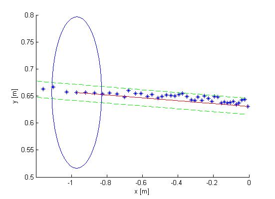
The next observation made from the Cartesian plot was that the data from the laser is actually quite noisy, as can be seen in Figure 2. The points do not align in a nice way, which can complicate decision making and mapping. One option is to make a fit over all the data points using basic functions for the walls instead of the points. This is also shown in Figure 2. If you assume that all the walls are straight (at least the walls are not substantially curved) you can use linear functions to represent the walls. If you do this in a correct manner you will only have to compare the robot position and orientation to the linear functions (i.e. only a zero order and first order constant a0 and a1) of these walls. Since you map only walls that are close to the robot this will reduce the input of your algorithms for wall avoidance from the number of laser points (over one thousand for the real life robot) to the first order functions of the walls (which will generally not exceed 8 wall segments, so 16 constants in total). A good motivation to continue developing an algorithm to do this.[[File:data_fit.jpg|400px|thumb|right|Figure 2: Data fit]] | |||
''' | |||
'''Mapping Algorithm''' | |||
The fitting of the lines over the data points is done in two steps. First the line start has to be found by making a start line. This start line is MIN_LENGTH_LINE points long. This number can changed be to make the algorithm more robust; here a minimal length of 4 points was chosen. The requirements for the line start are: | |||
* The points between the first and last point of the start line will have to lie closer to the line fitted between the first and last point of the start than the offset MAXIMAL_OFFSET_EVAL_LINE. This is shown in Figure 2. | |||
* The first and last point of the start line have to lie inside the relevant range of the robot discussed above (not too far and not on the robot itself). However, to avoid that one outlier prevents a line fit, it is allowed that one point falls outside the region of interest. This gives better performance than adjusting the allowed offset since this will give implications when a corner has to be mapped. Therefore all points should lie in between the offsets of the line. | |||
''' | |||
The | If these conditions are not met, no start line can be made and the search repeats, now with the next data point as starting point. If the start conditions are met, the line between the first and last point of the start line can be appended. This is done by checking if the next data point can replace the end point of the line that is appended. In order to do this, similar conditions have to be met as for the search of the start line, and the point has to lie between the same offset. Furthermore the line has to lie inside a certain region around the end point to be replaced, denoted as the circle in Figure 2. If the conditions are not met we do not append the line and start searching for a new line with the algorithm described above. However, to map lines at the edge of your region of interest, only if LINE_UNCERT_COUNT points in a row lie outside the region of interest we start looking for a new line (a value of 5 points was chosen). This is done to prevent that if a few points lie outside the region of interest but the wall actually continues the algorithm starts looking for a new line while it can easily continue appending the line it already found. [[File:merge_lines.jpg|400px|thumb|right|Figure 3: merge of lines]] | ||
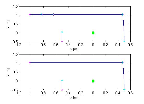
With this mapping algorithm the walls are not perfectly mapped. Some walls are split into two lines. One possible solution for this is to change the offset allowed for the points to be added to a line. However, this can cause the algorithm to miss corners easier. This problem was therefore solved by merging lines which clearly fit the same walls. To achieve this the distance between the end point of one line and the start point of the next line have to lie close to each other (maximum of MAXIMAL_DISTANCE_LINE_MERGE meters, an educated estimate of 0.2 m was chosen). Furthermore the slopes of the lines need to be close to each other. One problem that arises is that two lines of a wall parallel to the orientation of the robot can have a very positive slope, or a very negative slope. To account for this fact the slopes are converted to angles relative to the x-axis. If the angles differ less than π/6 rad and the end point and start point are close enough to each other the lines are merged. Since all corners in the maze are roughly π/2 it is not likely that two lines depicting a corner are seen as one wall and merged. Figure 3 shows the merging process. | |||
==Detection of the environment== | |||
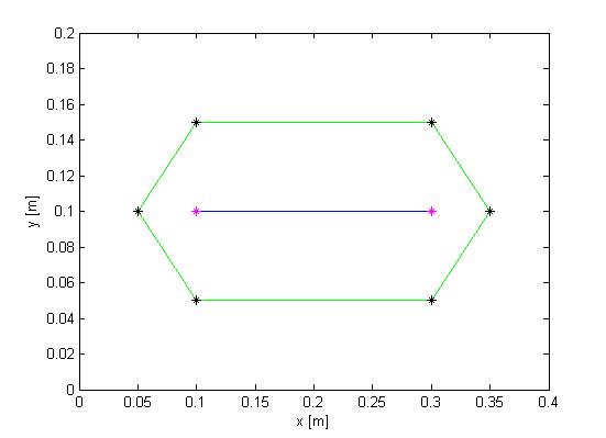
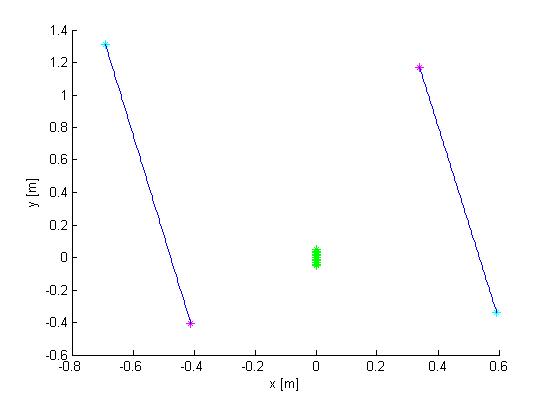
Figure 3 gives the output of the mapping strategy: all walls are represented by one line. The next step is now to find the position of these walls relative to the robot and find out whether these lines are of such importance that the robot needs to undertake action. For this a part of the code that was used for finding out whether a point was between certain offsets of a line was recycled. Replacing the laser point position with the robot position (which is always positioned at the origin) and adjusting the offset this makes an easy check to see whether a robot is close to a line and if a reaction is required. However, the recycled mapping algorithm does not take the distance to the start or end of the line into account. As long as the laser point is inside the region of interest and between the offsets the point is added. Now however, the robot should be close to the actual wall and not stand close to the extension of the line. An additional condition was added: the x or y position of the robot should line between the x or y positions of the start and end points of the line, taking an additional offset into account. Figure 4 shows the region that was checked. | |||
[[File:wall_proximity.jpg|300px|thumb|right|Figure 4: Wall proximity]] | |||
[[File:wall_alignment.jpg|300px|thumb|right|Figure 5: Wall alignment]] | |||
This gives the baseline for the most important algorithm in the code: wall avoidance. If the robot comes in the region depicted in Figure 4 it should stop moving and make a very wise decision to not crash into the wall. Steering away from the wall is such wise decision, and using the angle of the wall relative to the robot it can turn away from the wall and face free space. This is an ultimate situation, when the robot’s initial position is very close to the wall or the steering algorithm failed working. However, in the desired situation a wall alignment algorithm together with the algorithm for steering into openings should prevent such situation to occur. Since the coordinate system is located at the back of the robot a relative large distance needs to be maintained from the walls to prevent the front of the robot colliding into a wall. However, when taking corners it is possible that the back of the robot comes near a wall but there is no danger of collision, since the robot is not moving towards this wall. To prevent this from happening the distance that needs to be maintained from every wall is chosen such that the robot can come quite close to the wall but never touching it. However, this distance is too small to allow the robot to rotate. This has been solved by letting the robot drive backwards for a short time until the clearance from the wall is larger than the turning circle, and the robot can turn away from the wall with the same angle of reflection as the original angle of incidence was. | |||
'''Alignment''' | |||
In the normal situation, the previous section of wall avoidance should not be executed, since the alignment of the robot should be such that a safe distance from the wall is maintained. Wall alignment starts by finding the two walls in between which the robot is driving. This is done by finding all line fits that have a roughly the same angle to the x-axis, which would mean the lines are parallel to each other and can form a corridor. A second requirement for the lines is that the robot is positioned in between them and thus these lines are the corridor the robot is currently positioned in. To check if a line is next to the robot either the x-position or the y-position of the start and end point of the line has to have opposite line assuring that the line crosses the y-axis or x-axis respectively. Figure 5 shows such situation, where both lines have a similar angle to the x-axis (within π/6 rad difference) and both cross the x-axis. | |||
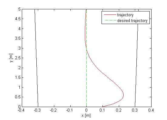
Once the walls next to the robot are detected a correction can be made. This correction will be a steering action and is based on two inputs: the angle of the robot relative to the walls and the position of the robot to both walls. To anticipate on the fact that the walls are usually not perfectly parallel the algorithm designs a desired trajectory. This trajectory is positioned right in between the two lines as depicted in Figure 6. Now the angle of the orientation of the robot to this desired trajectory and perpendicular distance can be calculated. Maintaining an equal forward velocity the calculated angle represents the velocity towards or away from the desired trajectory or the derivative of the position error, the perpendicular distance represents the total error in position. This problem can be solved using a PD controller where the P-action compensates for the position and the D-action for the orientation. Figure 6 shows the trajectory when such controller is implemented. The y-axis is the desired trajectory. | |||
[[File: PD-Trajectory.jpg|400px|thumb|right|Figure 6: PD controlled trajectory]] | |||
'''Corners''' | |||
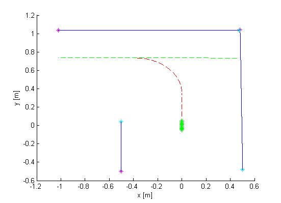
With the alignment and wall avoidance algorithm the robot can safely move between two walls. The next challenge is to ride safe when the robot is not between two walls and has to turn into an opening next to him. Figure 7 gives such situation, and the first problem to tackle is how to detect this situation. One thing that can be noticed is that in this situation there will always be two perpendicular lines marking the corner. Furthermore the end point of the first line will have to lie close to the start point of the second line. Finally, again both lines should cross either the x-axis or y-axis to make sure the lines are next to the robot, and see what direction is open by checking the slopes of the two lines. Using this information a desired trajectory for making the turn can be made. This is done by selecting a fixed distance the robot should stay from the wall you are facing once the turn is made and using the orientation and position calculating the needed angular velocity and turn time that would be required to get to this position. First however the robot drives a bit further into the maze to prevent collisions. Similarly, once the turn has been made, the robot drives straight until it detects two walls to align to. Figure 7 shows how a corner is taken. | |||
[[File: Corner_cross.jpg|400px|thumb|right|Figure 7: Crossing a corner]] | |||
'''Crossing Detection''' | |||
In a similar fashion as the corner detection a general crossing with more than one exits is detected. First two perpendicular lines have to be found, this time however the lines do not cross the x-axis or y-axis. Now a check is performed to see whether there are exits that are blocked or if it is a crossing with 3 exits. This is done by first assuming that all options (left, front and right) are open, and checking for all lines found whether they block the robot in one of the three directions. In the code used for the final competition based on this information the decision to turn into a crossing was already made based on priority of directions. If left is open turn left; else if straight ahead is open go straight; else take right. This wall follower algorithm is good for solving basic mazes. | |||
==Maze Solving Algorithm== | |||
Using the algorithms above the robot is to move through a maze that can be solved using a wall follower technique. To achieve the final goal: "Solving any maze as efficient as possible" a more extensive maze solving algorithm is needed. This algorithm was written in C++ code, but due to lack of time it was not implemented into the working code. | |||
The basic idea of the algorithm is that when a crossing is detected, a number of properties of this crossing will be saved into a node. With all the nodes (crossings) the robot creates, it builds a tree. Since implementing trees in a C++ code is quite difficult a structure system was used. The resulting structures then consists of: | |||
* node_id; This is the id of the crossing the robot just detected | |||
* x,y; These are the coordinates of the crossing, defined by the distance the robot drove from the start (this is not effecient but a better idea will be explained later) | |||
* parent; This is the node the robot previously visited. | |||
* child_right, child_front, child_left; The maximum amount of exits the robot could take on a crossing is 4 (inclusive the parent). | |||
The parent and the children are arrays which contain: | |||
* the node id of this parent; | |||
* the number of times the robot already crossed this path; | |||
* and a number which indicates whether this is the parent, left, right or front child. | |||
Furthermore there is a vector defined which contains all the nodes. | |||
When a crossing is detected the first thing the robot does is checking if it already visited this node. When this is the case he can just use the data from the previous time it was on this crossing. To make the algorithm a bit more accurate it was assumed that there will not be 2 crossings within in a radius of 1 meter. This to prevent the robot from making a new crossing node when it enters a crossing it visited before from another side. | |||
Like earlier mentioned, it is not accurate to use the odometry from the start to define coordinates for crossings. This is why for each crossing a new coordinate system is defined, where the origin is defined in the coordinate system of the previous crossing. All together this would result in a Tremaux algorithm for maze solving. One addition was made: when a crossing is found that was never visited before the preferred direction is straight ahead since this is the most convenient direction for the robot. What now remains is a combination of the Tremaux algorithm together with an dept-first-search maze solving algorithm. | |||
==Final results== | |||
The final algorithm worked pretty nice on the simulator. Corners were made, junctions were detected and the right wall was followed. The first youtube video shows the robot driving through a corridor with corners. The second video shows how the maze is solved. However, the algorithm lacked robustness. This is clearly seen at the end of the second movie. The robot sees the right direction options (left and right) and picks right, but the line for alignment after the corner is not correct and the robot does not turn enough and collision avoidance is activated. The second video shows that this position is no repeating error position. Unfortunately there was not enough time to fine-tune the code even more. | |||
* http://youtu.be/w-tfo6AdJRg | |||
* http://youtu.be/huVfGGtRYQk | |||
* http://youtu.be/tOqWldxNuhQ | |||
Latest revision as of 11:39, 6 July 2012
Group Info
| Group Members | Student nr. | |
| Christiaan Gootzen | c.f.t.m.gootzen@student.tue.nl | 0655133 |
| Sander van Zundert | a.w.v.zundert@student.tue.nl | 0650545 |
Tutor
Sjoerd van den Dries - s.v.d.dries@tue.nl
Due to major personnel changes the project was reset in week 7, and a brand new start was made. The results from this point on are reported in the section below.
The project was split into two parts. The first part consists of the basic robot control algorithm. This includes the mapping of the laser data in combination with odometry. With this alignment functions and wall avoidance can be implemented, as well as recognition of corners and junctions. The recognition of a junction marks the jump to the second part of the algorithm: solving the maze. For the corridor competition it is enough to find the first exit and leave the corridor: in the maze the decision making will start at the detection of the junction. The basic robot control algorithm consists of three separate points: data acquisition and simplification of the data, detection of the environment and the response of the robot to the environment.
Data acquisition and simplification
The laser-output from the robot is given in polar coordinates. The first thing done was to make a conversion to Cartesian coordinates to get a better feeling of how to treat the data, and the possibilities this would give for simplification of the data. For this conversion the following data was used:
- msg->ranges.size()
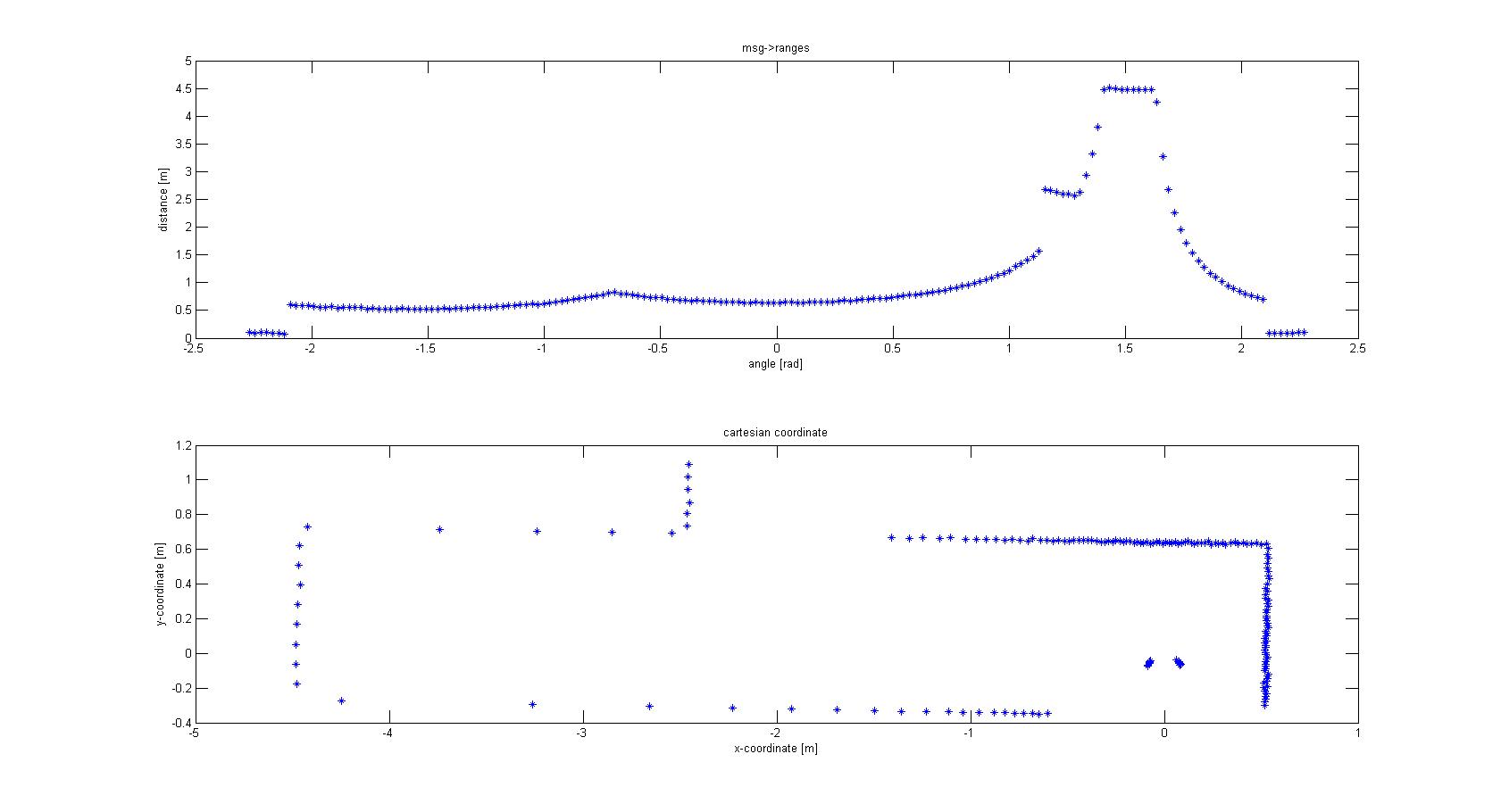
Figure 1: Data conversion - msg->angle_min
- msg->angle_max
- msg->ranges[x]; x < ranges->size()
- msg->angle_increment
With basic algebra the conversion was made, which is shown in Figure 1.
From the Cartesian plot some decisions can already be made. For instance, the data points that are plotted near the robot will have to be removed, since these are laser points that are projected on the robot itself. Furthermore we see a lot of points that are far away from the robot, all at a distance close to 10 meter. This is the maximum range of the laser points on the simulated robot, but on the real robot this might be different and can give a disturbing input. Therefore the data points which are relevant to the robot is limited to a range of TOO_FAR_TO_MAP meters, which is a static float to be fine-tuned to achieve good vision for the robot without large disturbances or processing time (limiting the data points you take into consideration when making decisions can speed up calculation times). Here a value of 1.5 meters was chosen.
The next observation made from the Cartesian plot was that the data from the laser is actually quite noisy, as can be seen in Figure 2. The points do not align in a nice way, which can complicate decision making and mapping. One option is to make a fit over all the data points using basic functions for the walls instead of the points. This is also shown in Figure 2. If you assume that all the walls are straight (at least the walls are not substantially curved) you can use linear functions to represent the walls. If you do this in a correct manner you will only have to compare the robot position and orientation to the linear functions (i.e. only a zero order and first order constant a0 and a1) of these walls. Since you map only walls that are close to the robot this will reduce the input of your algorithms for wall avoidance from the number of laser points (over one thousand for the real life robot) to the first order functions of the walls (which will generally not exceed 8 wall segments, so 16 constants in total). A good motivation to continue developing an algorithm to do this.
Mapping Algorithm
The fitting of the lines over the data points is done in two steps. First the line start has to be found by making a start line. This start line is MIN_LENGTH_LINE points long. This number can changed be to make the algorithm more robust; here a minimal length of 4 points was chosen. The requirements for the line start are:
- The points between the first and last point of the start line will have to lie closer to the line fitted between the first and last point of the start than the offset MAXIMAL_OFFSET_EVAL_LINE. This is shown in Figure 2.
- The first and last point of the start line have to lie inside the relevant range of the robot discussed above (not too far and not on the robot itself). However, to avoid that one outlier prevents a line fit, it is allowed that one point falls outside the region of interest. This gives better performance than adjusting the allowed offset since this will give implications when a corner has to be mapped. Therefore all points should lie in between the offsets of the line.
If these conditions are not met, no start line can be made and the search repeats, now with the next data point as starting point. If the start conditions are met, the line between the first and last point of the start line can be appended. This is done by checking if the next data point can replace the end point of the line that is appended. In order to do this, similar conditions have to be met as for the search of the start line, and the point has to lie between the same offset. Furthermore the line has to lie inside a certain region around the end point to be replaced, denoted as the circle in Figure 2. If the conditions are not met we do not append the line and start searching for a new line with the algorithm described above. However, to map lines at the edge of your region of interest, only if LINE_UNCERT_COUNT points in a row lie outside the region of interest we start looking for a new line (a value of 5 points was chosen). This is done to prevent that if a few points lie outside the region of interest but the wall actually continues the algorithm starts looking for a new line while it can easily continue appending the line it already found.
With this mapping algorithm the walls are not perfectly mapped. Some walls are split into two lines. One possible solution for this is to change the offset allowed for the points to be added to a line. However, this can cause the algorithm to miss corners easier. This problem was therefore solved by merging lines which clearly fit the same walls. To achieve this the distance between the end point of one line and the start point of the next line have to lie close to each other (maximum of MAXIMAL_DISTANCE_LINE_MERGE meters, an educated estimate of 0.2 m was chosen). Furthermore the slopes of the lines need to be close to each other. One problem that arises is that two lines of a wall parallel to the orientation of the robot can have a very positive slope, or a very negative slope. To account for this fact the slopes are converted to angles relative to the x-axis. If the angles differ less than π/6 rad and the end point and start point are close enough to each other the lines are merged. Since all corners in the maze are roughly π/2 it is not likely that two lines depicting a corner are seen as one wall and merged. Figure 3 shows the merging process.
Detection of the environment
Figure 3 gives the output of the mapping strategy: all walls are represented by one line. The next step is now to find the position of these walls relative to the robot and find out whether these lines are of such importance that the robot needs to undertake action. For this a part of the code that was used for finding out whether a point was between certain offsets of a line was recycled. Replacing the laser point position with the robot position (which is always positioned at the origin) and adjusting the offset this makes an easy check to see whether a robot is close to a line and if a reaction is required. However, the recycled mapping algorithm does not take the distance to the start or end of the line into account. As long as the laser point is inside the region of interest and between the offsets the point is added. Now however, the robot should be close to the actual wall and not stand close to the extension of the line. An additional condition was added: the x or y position of the robot should line between the x or y positions of the start and end points of the line, taking an additional offset into account. Figure 4 shows the region that was checked.
This gives the baseline for the most important algorithm in the code: wall avoidance. If the robot comes in the region depicted in Figure 4 it should stop moving and make a very wise decision to not crash into the wall. Steering away from the wall is such wise decision, and using the angle of the wall relative to the robot it can turn away from the wall and face free space. This is an ultimate situation, when the robot’s initial position is very close to the wall or the steering algorithm failed working. However, in the desired situation a wall alignment algorithm together with the algorithm for steering into openings should prevent such situation to occur. Since the coordinate system is located at the back of the robot a relative large distance needs to be maintained from the walls to prevent the front of the robot colliding into a wall. However, when taking corners it is possible that the back of the robot comes near a wall but there is no danger of collision, since the robot is not moving towards this wall. To prevent this from happening the distance that needs to be maintained from every wall is chosen such that the robot can come quite close to the wall but never touching it. However, this distance is too small to allow the robot to rotate. This has been solved by letting the robot drive backwards for a short time until the clearance from the wall is larger than the turning circle, and the robot can turn away from the wall with the same angle of reflection as the original angle of incidence was.
Alignment
In the normal situation, the previous section of wall avoidance should not be executed, since the alignment of the robot should be such that a safe distance from the wall is maintained. Wall alignment starts by finding the two walls in between which the robot is driving. This is done by finding all line fits that have a roughly the same angle to the x-axis, which would mean the lines are parallel to each other and can form a corridor. A second requirement for the lines is that the robot is positioned in between them and thus these lines are the corridor the robot is currently positioned in. To check if a line is next to the robot either the x-position or the y-position of the start and end point of the line has to have opposite line assuring that the line crosses the y-axis or x-axis respectively. Figure 5 shows such situation, where both lines have a similar angle to the x-axis (within π/6 rad difference) and both cross the x-axis.
Once the walls next to the robot are detected a correction can be made. This correction will be a steering action and is based on two inputs: the angle of the robot relative to the walls and the position of the robot to both walls. To anticipate on the fact that the walls are usually not perfectly parallel the algorithm designs a desired trajectory. This trajectory is positioned right in between the two lines as depicted in Figure 6. Now the angle of the orientation of the robot to this desired trajectory and perpendicular distance can be calculated. Maintaining an equal forward velocity the calculated angle represents the velocity towards or away from the desired trajectory or the derivative of the position error, the perpendicular distance represents the total error in position. This problem can be solved using a PD controller where the P-action compensates for the position and the D-action for the orientation. Figure 6 shows the trajectory when such controller is implemented. The y-axis is the desired trajectory.
Corners
With the alignment and wall avoidance algorithm the robot can safely move between two walls. The next challenge is to ride safe when the robot is not between two walls and has to turn into an opening next to him. Figure 7 gives such situation, and the first problem to tackle is how to detect this situation. One thing that can be noticed is that in this situation there will always be two perpendicular lines marking the corner. Furthermore the end point of the first line will have to lie close to the start point of the second line. Finally, again both lines should cross either the x-axis or y-axis to make sure the lines are next to the robot, and see what direction is open by checking the slopes of the two lines. Using this information a desired trajectory for making the turn can be made. This is done by selecting a fixed distance the robot should stay from the wall you are facing once the turn is made and using the orientation and position calculating the needed angular velocity and turn time that would be required to get to this position. First however the robot drives a bit further into the maze to prevent collisions. Similarly, once the turn has been made, the robot drives straight until it detects two walls to align to. Figure 7 shows how a corner is taken.
Crossing Detection
In a similar fashion as the corner detection a general crossing with more than one exits is detected. First two perpendicular lines have to be found, this time however the lines do not cross the x-axis or y-axis. Now a check is performed to see whether there are exits that are blocked or if it is a crossing with 3 exits. This is done by first assuming that all options (left, front and right) are open, and checking for all lines found whether they block the robot in one of the three directions. In the code used for the final competition based on this information the decision to turn into a crossing was already made based on priority of directions. If left is open turn left; else if straight ahead is open go straight; else take right. This wall follower algorithm is good for solving basic mazes.
Maze Solving Algorithm
Using the algorithms above the robot is to move through a maze that can be solved using a wall follower technique. To achieve the final goal: "Solving any maze as efficient as possible" a more extensive maze solving algorithm is needed. This algorithm was written in C++ code, but due to lack of time it was not implemented into the working code.
The basic idea of the algorithm is that when a crossing is detected, a number of properties of this crossing will be saved into a node. With all the nodes (crossings) the robot creates, it builds a tree. Since implementing trees in a C++ code is quite difficult a structure system was used. The resulting structures then consists of:
- node_id; This is the id of the crossing the robot just detected
- x,y; These are the coordinates of the crossing, defined by the distance the robot drove from the start (this is not effecient but a better idea will be explained later)
- parent; This is the node the robot previously visited.
- child_right, child_front, child_left; The maximum amount of exits the robot could take on a crossing is 4 (inclusive the parent).
The parent and the children are arrays which contain:
- the node id of this parent;
- the number of times the robot already crossed this path;
- and a number which indicates whether this is the parent, left, right or front child.
Furthermore there is a vector defined which contains all the nodes.
When a crossing is detected the first thing the robot does is checking if it already visited this node. When this is the case he can just use the data from the previous time it was on this crossing. To make the algorithm a bit more accurate it was assumed that there will not be 2 crossings within in a radius of 1 meter. This to prevent the robot from making a new crossing node when it enters a crossing it visited before from another side.
Like earlier mentioned, it is not accurate to use the odometry from the start to define coordinates for crossings. This is why for each crossing a new coordinate system is defined, where the origin is defined in the coordinate system of the previous crossing. All together this would result in a Tremaux algorithm for maze solving. One addition was made: when a crossing is found that was never visited before the preferred direction is straight ahead since this is the most convenient direction for the robot. What now remains is a combination of the Tremaux algorithm together with an dept-first-search maze solving algorithm.
Final results
The final algorithm worked pretty nice on the simulator. Corners were made, junctions were detected and the right wall was followed. The first youtube video shows the robot driving through a corridor with corners. The second video shows how the maze is solved. However, the algorithm lacked robustness. This is clearly seen at the end of the second movie. The robot sees the right direction options (left and right) and picks right, but the line for alignment after the corner is not correct and the robot does not turn enough and collision avoidance is activated. The second video shows that this position is no repeating error position. Unfortunately there was not enough time to fine-tune the code even more.