Embedded Motion Control 2015 Group 6: Difference between revisions
No edit summary |
|||
| (125 intermediate revisions by 5 users not shown) | |||
| Line 1: | Line 1: | ||
= Group Members = | = '''Group Members''' = | ||
<table border="1" cellpadding="5" cellspacing="0" style="width:100%;border-collapse:collapse;"> | <table border="1" cellpadding="5" cellspacing="0" style="width:100%;border-collapse:collapse;"> | ||
<tr style="background: #D3D3D3;"> | <tr style="background: #D3D3D3;"> | ||
| Line 43: | Line 43: | ||
<!-- White space --> | <!-- White space --> | ||
= '''Initial Design''' = | = '''Initial Design''' = | ||
| Line 137: | Line 82: | ||
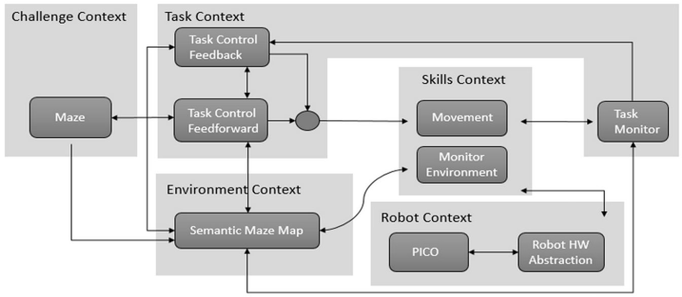
Initial Schematic overview of the components to be used in the software design | Initial Schematic overview of the components to be used in the software design | ||
[[File:Components. | [[File:Components image 2.JPG|frameless|upright=5|Environment detection: T-junction]] | ||
1) '''Task Context:''' Controls the implementation of the robots functions depending on the challenge and environmental context. | 1) '''Task Context:''' Controls the implementation of the robots functions depending on the challenge and environmental context. | ||
| Line 162: | Line 108: | ||
5) '''Task Context – Skill Context:''' Allocates the necessary skill dependent on the contribution of the task control feedforward and feedback. | 5) '''Task Context – Skill Context:''' Allocates the necessary skill dependent on the contribution of the task control feedforward and feedback. | ||
= '''Corridor Competition''' = | |||
For this competition, it was aimed to exit the corridor succesfully with an easy approach. | |||
== Hardware Components == | |||
* Wheels: | |||
** The robot doesnt move in a straight line when a move command is given in the x direction. This is because of the omniwheels which make the robot rotate whenever it moves forward. For this reason we need an allignment algorithm. | |||
* Laser Data: | |||
** The laser stores position information and angular information in laser data framework | |||
** Every laser needs to be calibrated and multiple lasers are used to get a homogenous result and trustable data. | |||
* Odometry Data: | |||
** Gives information about the relative changes in X, Y and angular position. The first navigation algorithm was based on this odometry data, but since good results were not obtained, it was changed by using laserdata. | |||
== Initial Software Design == | |||
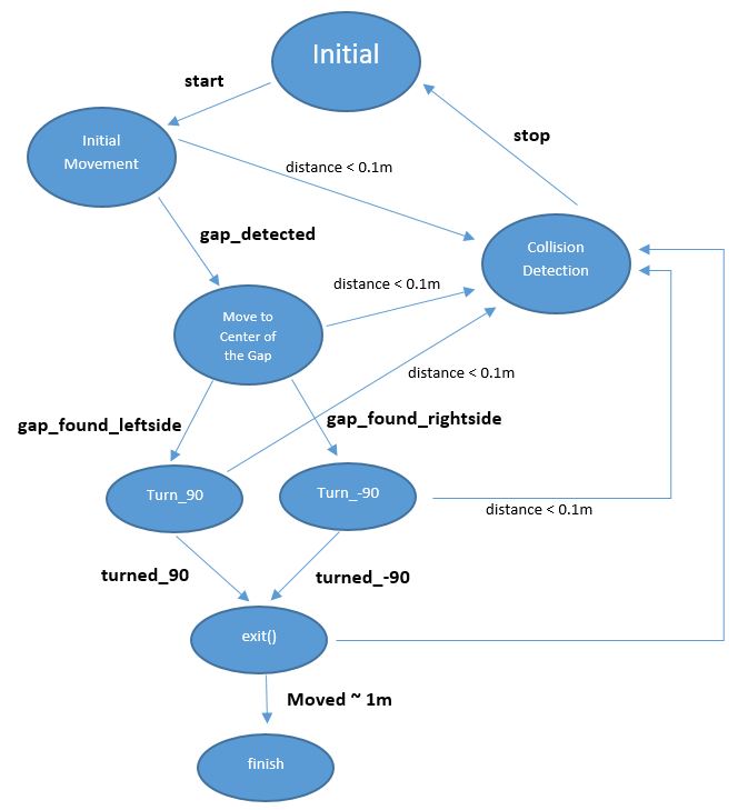
* Initial Movement: Robot starts with a constant speed and move forward through the corridor. | |||
* Collision Detection: With using the laser data, distance to the wall or any other obstacles (no obstacles in this case) can be determined. If the distance becomes less than 0.1 metre, robot will stop to avoid collision. | |||
* Position Alignment: It is observed that, due to feature of omni wheels, robot sometimes can not go straight. So in the algorithm, Pico is forced to stay in the middle of the corridor by calculating the distance to the right and left wall by using laser data. | |||
* CheckCorridor: Robot will constantly check the distances to the left and right wall. If the distance to one of them exceeds the threshold (max.width has already known) turn left/right command will be executed. | |||
* Turn Left/Right: After robot moves in the middle of the gap, it turns +/-90 degrees by using the odometry data. When it is turned, it again starts moving forward. | |||
* Finish: Since the distance to finish can be approximated, after moving some distance, robot will stop automatically. | |||
States of the initial design can be seen in the following figure: | |||
[[File:InitialAlgorithm.JPG|center]] | |||
== Features of the Software == | |||
=== Collision Detection === | |||
When the distance between the robot and wall becomes smaller than 0.1 meters, initial collision detection function stop the robot before it hits the wall. This function will be upgraded further. | |||
=== Position Alignment === | |||
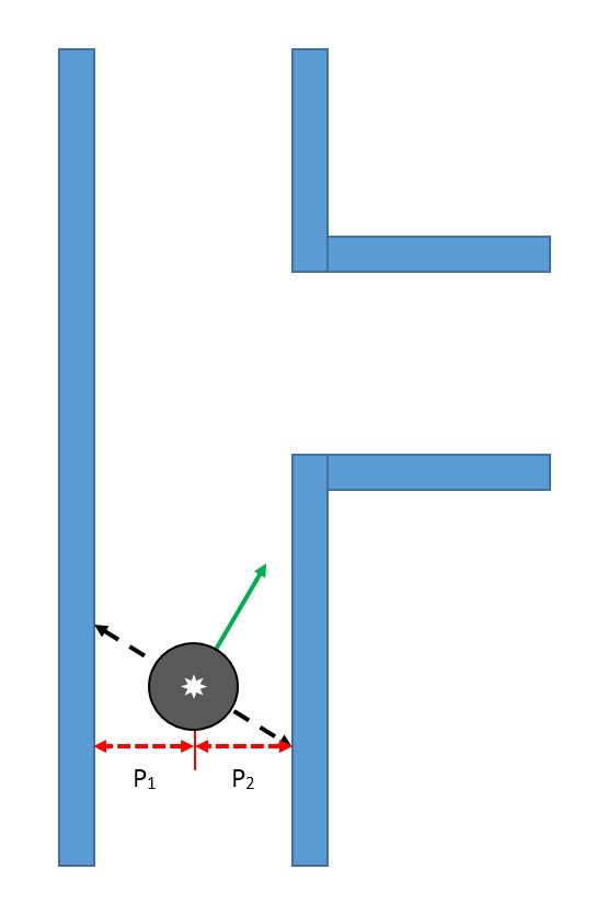
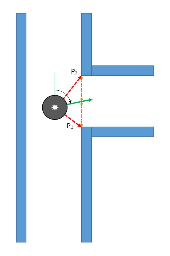
Pico looks at its environment and takes the information from the laserdata to calculate the distance to the walls. If the difference in distance to both left (P<sub>1</sub>) and right (P<sub>2</sub>) side of the wall is the minimum possible, then a perpendicular relation is found. This also means that pico is going in a straight line through the centre of the hallway. | |||
[[File:IMAGE 1 - Position Alignment.JPG|frameless|upright=1.5|Environment detection: T-junction]] | |||
=== Find the Gap === | |||
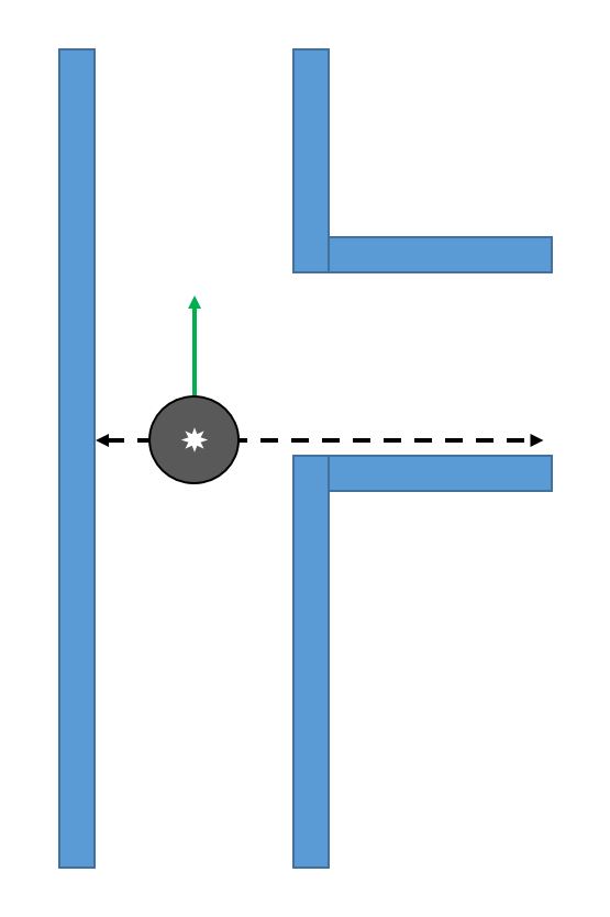
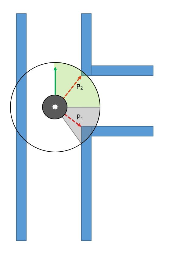
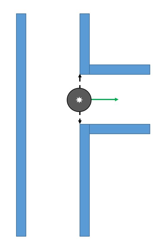
While moving forward the above condition is checked at every time step, correcting itself where necessary. When pico encounters a turn, one of the distance vectors will increase drastically. At that point, pico stops and looks at its environment. It calculates (in the direction of the increased vector) the shortest possible distance to the wall and saves this point as the rotation point. The other side of the gap is calculated by using the same technique, but in a different quadrant. The rotation radius is then the half of the distance between these two points. After the rotation is complete pico starts from the beginning again. | |||
[[File:IMAGE 2 - Find the Gap 1.JPG|frameless|upright=1.5|Environment detection: T-junction]] [[File:IMAGE 3 - Find the Gap 2 - V2.JPG|frameless|upright=1.5|Environment detection: T-junction]] [[File:IMAGE 4 - Find the Gap 3 - V2.JPG|frameless|upright=1.5|Environment detection: T-junction]] [[File:IMAGE 5 - Find the Gap 4.JPG|frameless|upright=1.5|Environment detection: T-junction]] | |||
== Tests before corridor competition and Updates to Software == | |||
The day before the corridor competition, our algorithm was tested on the robot 3 times. | |||
On the first try, the robot solved the maze. On the second try we noticed that although the robot was aligning its position to the centre, the robot's angle was slightly tilted | |||
from the "0" mean angle position. This angular tilt of the robot caused the robot to fail to finish the test run on the second and third try. | |||
Final amendment to code before corridor competition: The night prior to the competition we decided to amend the code and include an angular alignment function to eliminate | |||
the angular tilt. This code was tested on the simulation and it worked perfectly. | |||
== Analysis of the Competition == | |||
Corridor Competition: | |||
In the corridor competition, we were given 2 tries like every other group. On our first try, the robot did not move. We ran our code but | |||
the robot seemed to do nothing. There was no behaviour. | |||
On the second try, we asked the coordinator to reset the odometry data which he did and we ran our code. | |||
The robot moved roughly for 3 seconds and then stopped. | |||
Software bugs during the corridor competition. | |||
We had numerous bugs in our software during the competition. The first bug in our software was the angular | |||
alignment function we included the previous night. Due to haste, we used odometry data and a while loop in the code. The function | |||
checked if the odometry angle was at "0" mean. We defined 0 mean as odometry angle between 0.1 and -0.1. Anytime the odometry angle went above these angles while the robot was not turning, we | |||
sent the error back as a feedback to a while loop and used the error to determine if we were to align our angle in the x or y direction. This implementation worked on the simulation so we did | |||
not realise how infeasible this method was on the real system. The while loop ran at an "infinitely" higher frequency than the robot thus the odometry variables were not updated in real time. | |||
The second bug was from using odometry data constantly. Odometry data accumulates error overtime and returns very erroneous data which causes erratic behaviour. | |||
Reason for robot behaviour in first try: The odometry data accumulated error over time from the previous groups so when we ran our program, the odometry sent erroneous data as feedback thus the condition for the loop to break was never | |||
met which caused the robot to do nothing. | |||
Reason for robot behaviour in second try: After the coordinator reset the odometry data, we reran our code. The behaviour was caused by the while loop. After 3 seconds, the angular position moves away from the | |||
"0" mean angular position. The software logic moved into the while loop and got stuck in the while loop since the while loop runs "infinitely" faster than 40 Hz which the robot which runs at thus causing the | |||
variables never to be updated | |||
After the corridor competition, alignment was added to the code properly. The code can be seen below. Now the alignment has done by using just laser data. By updating the alignment, we were able to finish corridor competition. | |||
<code> | |||
void move_forward(bool move_status, global_state_monitor &state) | |||
{ | |||
io.readLaserData(scan); | |||
double left_dist_to_wall = scan.ranges[893]; //distance at +90 degrees | |||
double right_dist_to_wall = scan.ranges[107]; //distance at -90 degrees | |||
double align_diff = left_dist_to_wall-right_dist_to_wall; | |||
double closest_point_right = findmin(scan,1); | |||
double closest_point_left = findmin(scan,2); | |||
double angle_diff = (closest_point_right - 107)*0.004; | |||
if((abs(align_diff) < 0.08) || ( abs(align_diff) > 0.5) ){ | |||
align_diff = 0; | |||
} | |||
if((abs(angle_diff) < 0.008) || ( abs(align_diff) > 0.15)){ | |||
angle_diff = 0; | |||
} | |||
if(move_status) | |||
{ | |||
io.sendBaseReference(0.4, align_diff/2, angle_diff/6); | |||
} | |||
else | |||
{ | |||
io.sendBaseReference(0, 0, 0); | |||
} | |||
} | |||
</code> | |||
= '''Maze Competition''' = | |||
== Components and Specificications== | |||
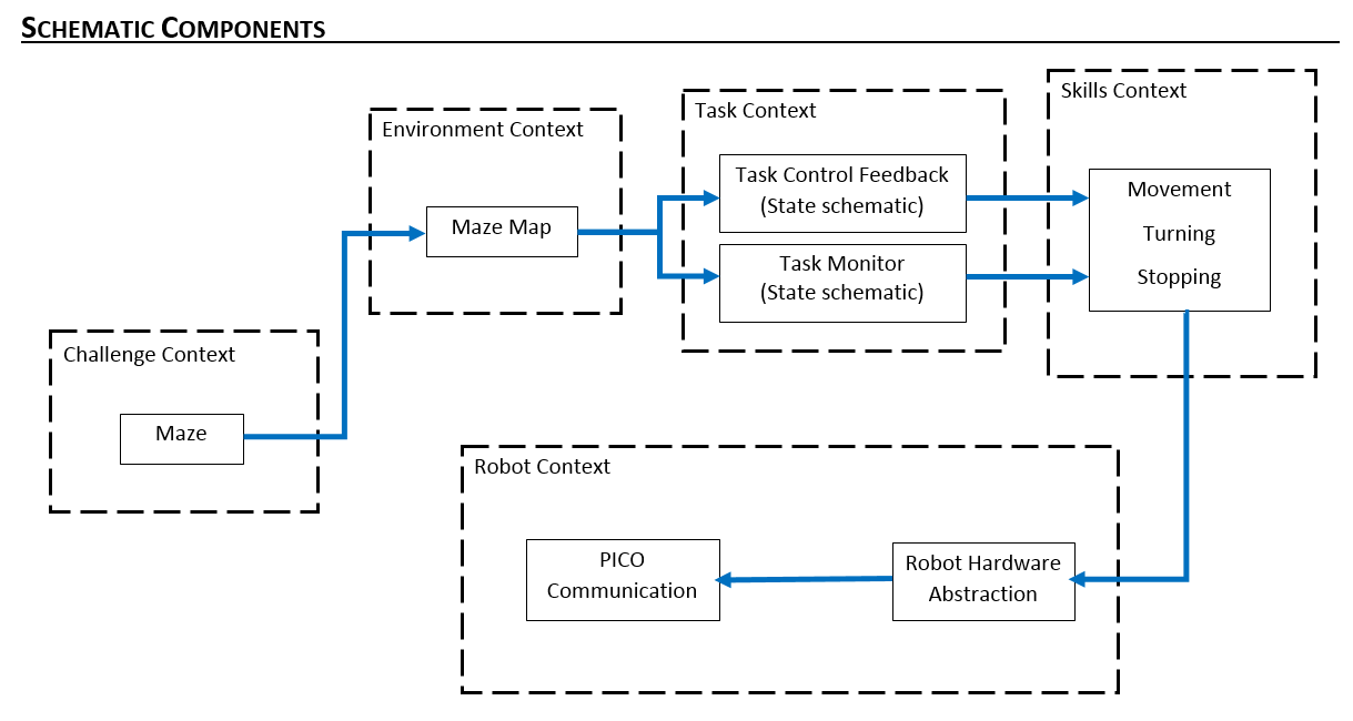
Initial Schematic overview of the components to be used in the software design | |||
[[File:Design maze.PNG|center]] | |||
== Interfaces == | |||
1) '''Environmental Context - Task Context:''' | |||
The task context identifies the geometric shape at the junction, and then places a node and saves the node's orientation, parents, and children. The information regarding the node is | |||
then passed back to the environmental context which then updates the the local map. Based on the type of junction encountered, the task monitor then sends this information to the skills context | |||
2) '''Task Context - Skills Context:''' | |||
The skills context then implements the particular robotic skill needed to traverse the geometric shape encountered. After the required skill is implemented, the information is sent back to the task context which then updates the task monitor. The task monitor then sends the information to the environmental context which updates the position of the robot in the maze. | |||
3) '''Skills Context - Robot Context:''' | |||
Dependent on the skills to be implemented, the code is sent to the low level robot context which then implements the particular behaviour wanted and passes the information back to the skills context | |||
4) '''Finite State Machine:''' | |||
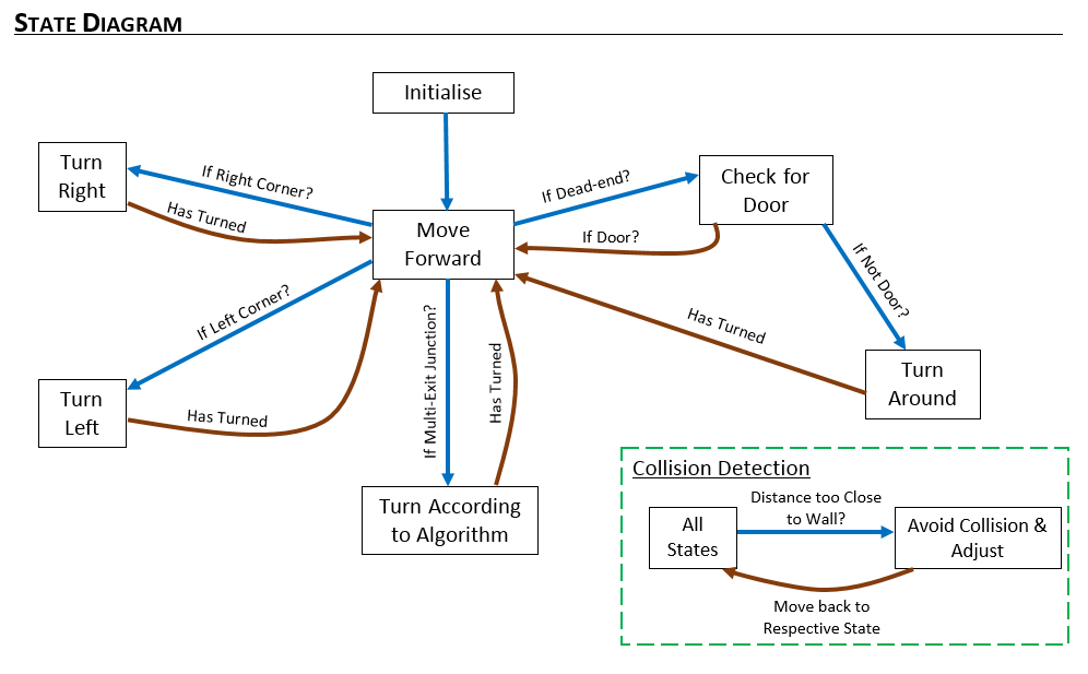
In order to navigate within the maze, a finite state machine (FSM) was implemented. The purpose of the FSM was to assign the right state which is dependent on the occurence of an event or multiple events. | |||
Below is the state diagram showing the transition between states. | |||
[[File:States.PNG|center]] | |||
From the diagram, it can be seen which respective event triggers a state. | |||
The events are | |||
* if right corner detected | |||
* if deadend detected | |||
* if door present | |||
* if door absent | |||
* has turned around | |||
* if right corner present | |||
* if left corner present | |||
* has turned | |||
* if multiple exit junction detected | |||
== Building our local Map == | |||
In this assignment, we thought about building a world map using the hector mapping library but encountered several issues with the importing. on further thought we decided to use a local map | |||
which will be built as we navigate through the maze. At the starting position of the maze we place a node with index 1 and store its orientation. On moving, when a junction (junction here meaning a geometric shape which would require the robot to change state) is encountered, another node is placed there storing its orientation, parent and children. Depending on the type of junction encountered, the second node will check the left, right and forward extreme of the junction and then store these positions as its children in the map. This process is continued till the entire map has been stored. | |||
== Algorithm == | |||
The algorithm we have adopted is a subset of the depth first search algorithm with the nodes placed at respective junctions. Each node comprises of a parent and several children.The children of the nodes are at the left and right extremes of the junction. When the robot moves down a desired path and encounters a dead end, the robot is then able to backtrack to the previous junction by moving to its parent. When a node is visited, this information is stored and used when searching for unexplored areas. This technique is not optimal as it focusses on navigating through the entire maze rather than searching for the optimal distance but it is more reliable as it makes sure it explores the entire span of the maze. Also anytime a node is visited, the index of the node is stored in the visited section thus enabling us to know when a node has been visited and thus enabling us to navigate through the maze without entering an infinite loop. | |||
=== Depth First Search === | |||
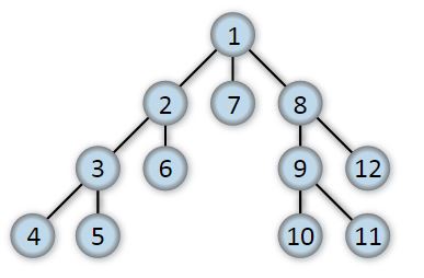
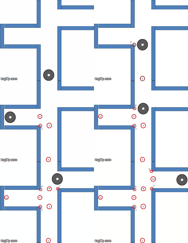
This algorithm is utilized for traversing tree/graph data structures. Starting at a root position, the algorithm moves through the tree along each possible branch before back-tracking. Although it is not considered the most efficient method for maze solving (unlike A*), for our intentions it is a more comprehensive system when compared other solving-algorithms. The image below shows a simple data structure that can be tackled with DFS. Starting at node 1, the algorithm then moves to 2, 3, and then 4, at which point it reaches the end of a branch. When this occurs the algorithm moves back to the previous node (in this case 3), and then attempts to take another branch (to node 5). This system continues throughout until the entire branch is mapped. | |||
[[File:DFS image.JPG|center|frameless|upright=2.5|Environment detection: T-junction]] | |||
When compared with a simple algorithm such as the “wall-follower” method (WFM), which follows either the left- or right-wall (depending on specifications in the code) to solve the maze, DFS can be considered more robust overall. This comes down to 2 factors: firstly, the WFM is considered one of the slowest methods (heavily dependent on the size of the maze and starting position); and secondly, the WFM is susceptible to entering a loop within the maze which it cannot exit. DFS on the other hand can be considered a slow method, but it is very unlikely to get caught in a loop due to the formation and tracking of nodes within the algorithm, as mentioned above.The gif below shows how DFS is utilised by PICO to solve the maze. | |||
[[File:Pico Animation.gif|center|frameless|upright=2.5|Environment detection: T-junction]] | |||
=== Top Level Decision === | |||
This is the "brain" in the robotic software. It issues commands in the software. Our algorithm to solve the maze focused on building a maze tree obtained by the geometric shapes in the local map (corners, deadends, etc), such as in the gif above. The global state monitor (GSM) made sure our algorithm was strictly adhered to. The monitors aim was for the robot to navigate through all the nodes until the exit is found. | |||
==== How the "Brain" works ==== | |||
When the robot starts the system is initiated. After initialisation the GSM calls the "move forward" function. The state remains in "move forward" until the robot comes across a geometric junction. The GSM then calls the "detect geometric shape" function to identify which shape has been encountered. Depending on the determined shape, a specific event is triggered. When the event is triggered the GSM changes the state of the final state machine. | |||
==== Event ==== | |||
If a right corner is detected → By our definition of right turn, only one possible movement is possible, which is the "right turn" geometry. The GSM then changes the state to "right turn". | |||
If a left corner is detected → The same occurs as in the right turn, with the state being changed to "left turn" instead. | |||
If deadend → The state is changed to check for door. If a door is found (waiting for 5 seconds and detecting an exit), the state is changed to "beep and move forward". If no door is present, the state is changed to "turn around". | |||
If a multiple junction exit is detected → Depending on the information from the maze tree, the GSM calls the state which turns according to the information. | |||
=== Code Interaction === | |||
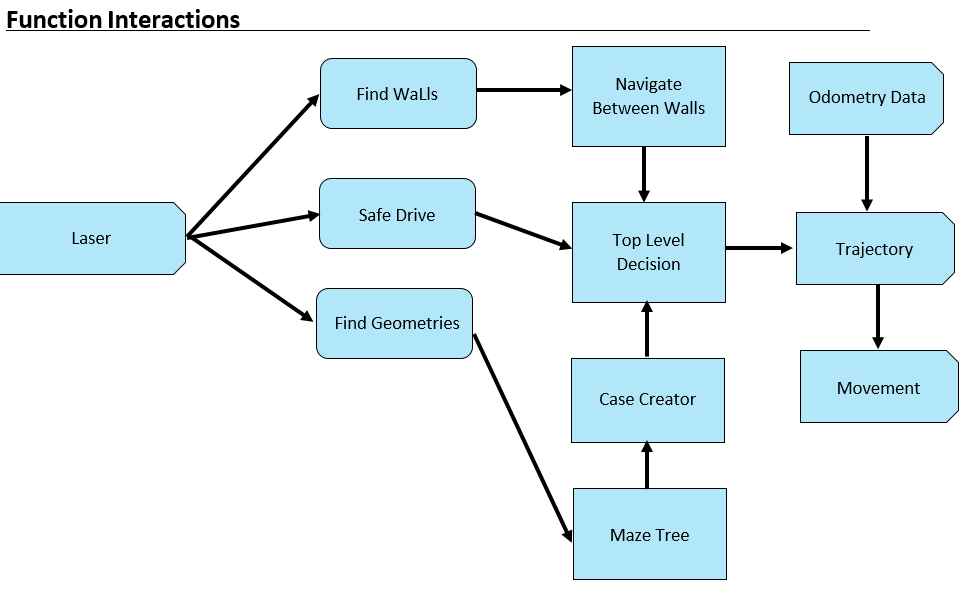
The main program uses some defined robot functionalities in order to achieve its goal. Below, interaction of all functions and global ros input variables can be seen. | |||
[[File:Interactions.PNG|center]] | |||
==== Find Geometries ==== | |||
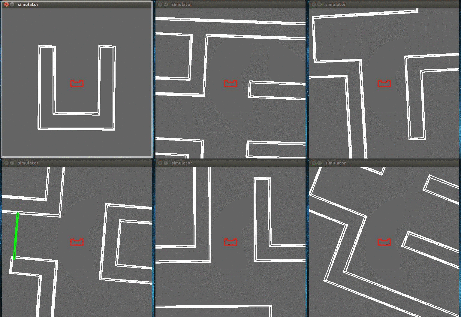
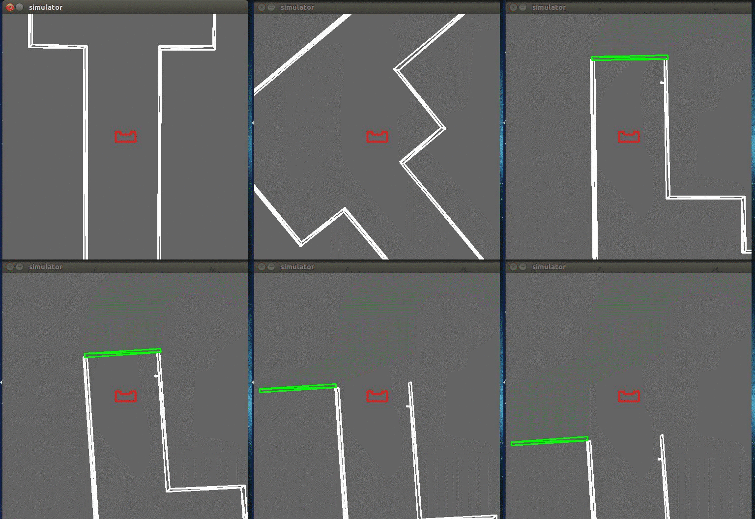
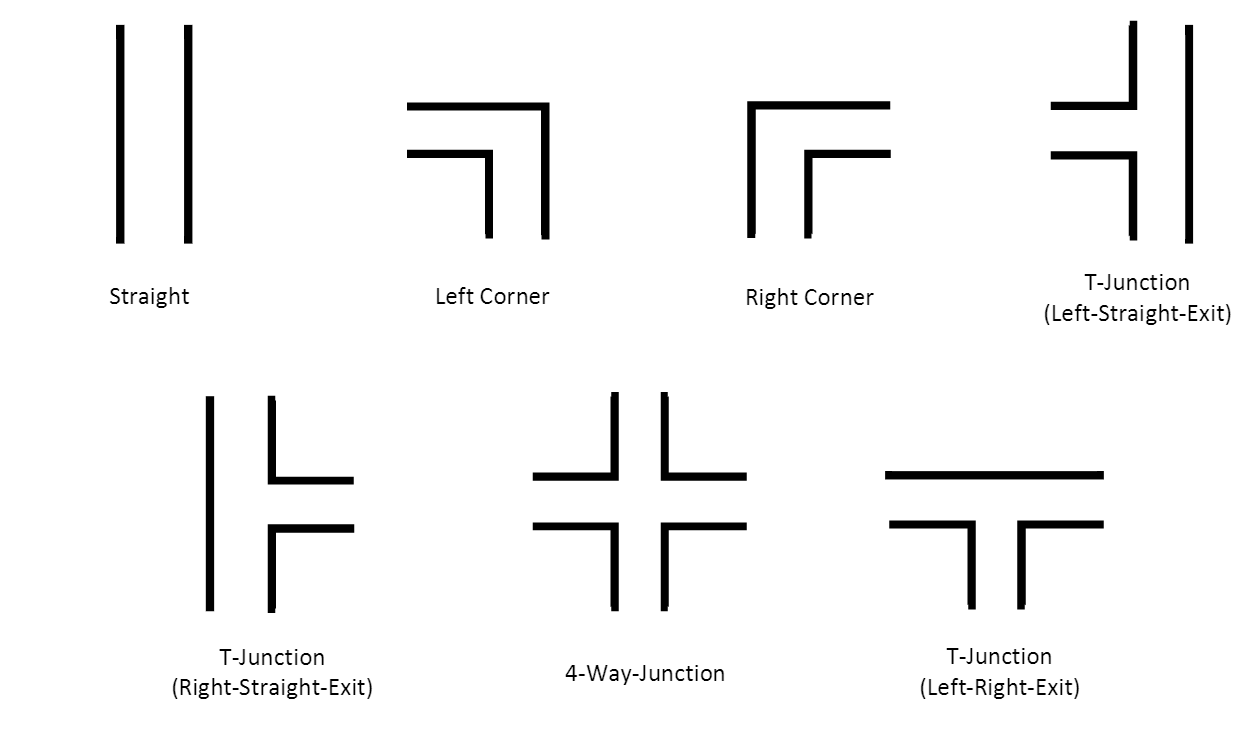
The robot should be able to recognize all possible geometries in order to navigate through the maze. State changes will be determined by detected geometries while the robot is moving. | |||
Defined geometries are shown belown: | |||
[[File:Shapes.PNG|center|frameless|upright=3.5|Environment detection: T-junction]] | |||
==== Main Algorithm: ==== | |||
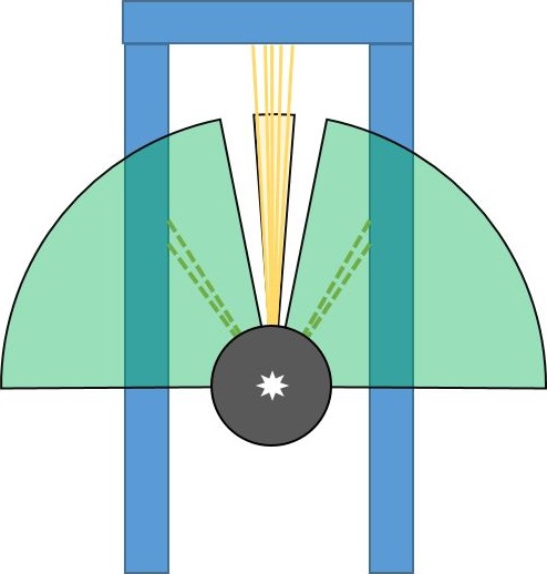
* Start scanning the environment from -90 to 90 degrees with respect to the robot. Pico's view is separated as left, middle and right. Middle view is responsible for measuring the distance in front of Pico. Therefore this distance is calculated by using range of points inside the middle view in order to get more reliable result. Left and right views are responsible for the detection of edges in front of the Pico. Views can be seen at the figure below: | |||
[[File:Image_1_-_PICO_Field_of_View.JPG|frameless|upright=2.5|Environment detection: T-junction]] | |||
* First edges of the geometries are found by comparing all consecutive elements in the left and right views. | |||
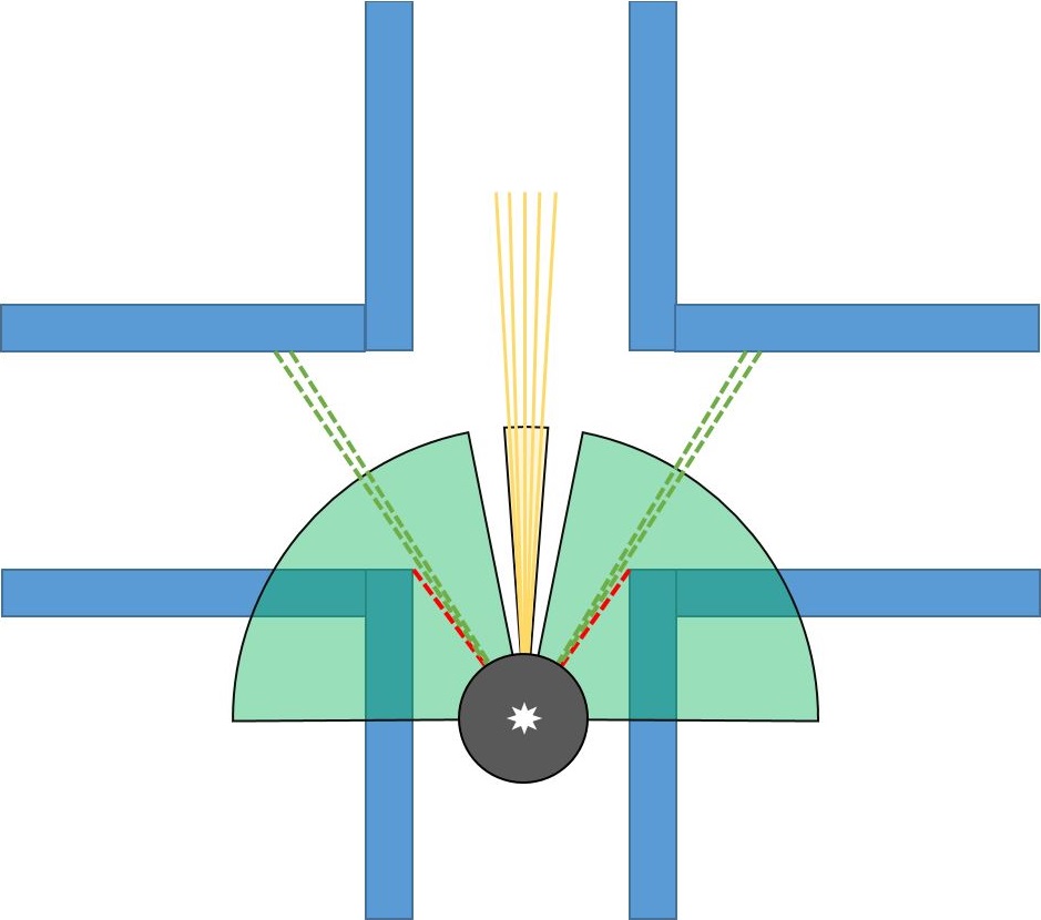
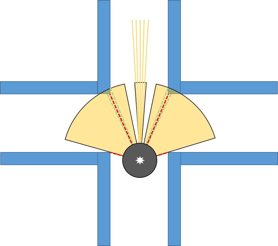
* All points [i] in the separated views are compared with next two consecutive beams. At the figure left below, the red dashed line will be compared with next laser data in terms of distance and since the difference in distance between first point and next points is higher than the threshold, this point will be accepted as edge. | |||
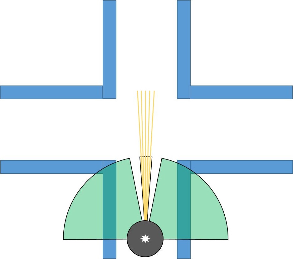
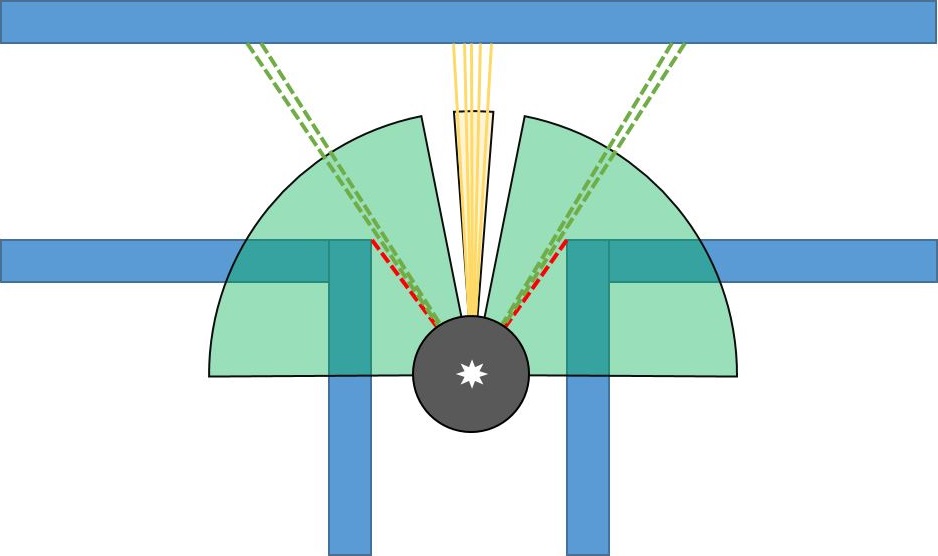
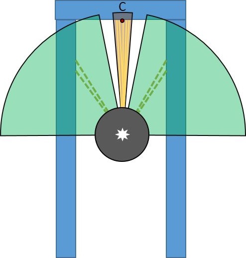
* For the corridors, there will be a second edge. This can be found by continue scanning left/right views starting from the angle of the first edge. In this range, the smallest point to the robot will be our second edge. Threshold is given for the distance between these points. If the distance between first edge and second is smaller than this threshold, that means the found geometry is just a hole. Otherwise, the edges are saved as an element for the corridors. At the figure right below, new view is defined as yellow area, and the most closest point to the robot in that area is accepted as second edge. | |||
[[File:Image 2 - PICO at 4-Way-Junction.JPG|frameless|upright=2.5|Environment detection: T-junction]] [[File:Image 3 - PICO in 4-Way-Junction.JPG|frameless|upright=2.5|Environment detection: T-junction]] | |||
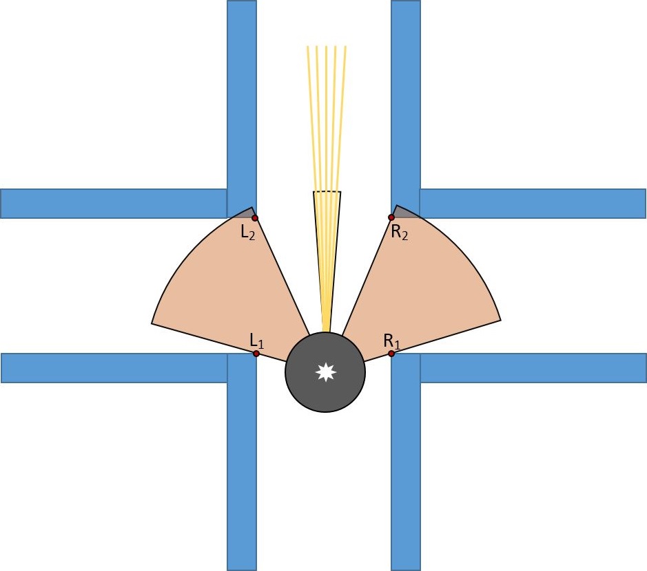
* Found edges can be seen at figure belown. If l1 and l2 edges are found that means the robot is encountered with left corridor, if r1 and r2 edges are found that means the robot is encountered with right corridor and if both l1, l2, r1 and r2 edges are found that means the robot is encountered with 4-way junction. | |||
[[File:Image 4 - PICO defined 4-Way-Junction corners.JPG|frameless|upright=2.5|Environment detection: T-junction]] | |||
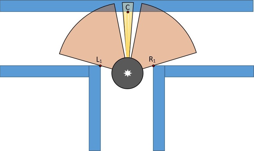
* For the corners, there won't be a second edge. If the first edge is found and the front distance (that is calculated before by using middle view) is lower than the defied threshold, that means the found edge belongs to a left/right corner. If C1,L1 and R1 is found that means that the robot is encountered with t-junction. C1 is saved as point when the calculated distance of the robot front view is lower than the threshold. In that way we can detect whether the detected shape is corridor or corner. | |||
[[File:Image 5 - PICO in T-Junction.JPG|frameless|upright=2.5|Environment detection: T-junction]] [[File:Image 6 - PICO defined T-Junction corners.JPG|frameless|upright=2.5|Environment detection: T-junction]] | |||
The following is the code for the left corridor check. | |||
<code> | |||
void LeftCorridorCheck(point (&left_cor)[2], global_state_monitor &state,geometric_shapes &shapes,double &left_corridor_exist){ | |||
io.readLaserData(scan); | |||
double min=1000; | |||
double index_second_corner=0; | |||
double index_first_corner=0; | |||
for(unsigned int i = 893; i > 650;i--){ | |||
if( abs(scan.ranges[i-1]-scan.ranges[i] && abs(scan.ranges[i-2]-scan.ranges[i]) > 0.1){ // finds the first edge by comparing near points | |||
//cout << "corridor is detected on the left. first phase " << i << endl; | |||
index_first_corner = i; | |||
break; | |||
} | |||
} | |||
if(index_first_corner > 0){ // if the first edge is found, then look for a second edge and find it. | |||
for(unsigned int j = index_first_corner-1; j > 510;j--){ | |||
if((abs(scan.ranges[j]) < min) && (scan.ranges[j] > 0.1)){ | |||
min = scan.ranges[j]; | |||
index_second_corner = j; | |||
} | |||
} | |||
if(abs(index_first_corner - index_second_corner) > 40){ // if the index between the edges smaller than 40, it means that is gap otherwise it will be saved as left corridor | |||
left_cor[1].angle = index_first_corner; | |||
left_cor[1].distance = scan.ranges[index_first_corner]; | |||
left_cor[2].angle = index_second_corner; | |||
left_cor[2].distance = scan.ranges[index_second_corner]; | |||
shapes.T_crossing_left_straight = true; | |||
left_corridor_exist = true; | |||
} | |||
else{ | |||
left_cor[1].angle = 0; | |||
left_cor[1].distance = 0; | |||
left_cor[2].angle = 0; | |||
left_cor[2].distance = 0; | |||
} | |||
} | |||
} | |||
</code> | |||
===== Special Case: DeadEnd ===== | |||
The deadend occurs when no edges are found and the front of the robot is blocked (smaller than specified threshold). Then the robot waits for 5 seconds and again checks the distance to determine if it is still a deadend or if it has become an exit. If it is an exit, PICO continues moving forward. If it is a deadend the robot then turns 180<sup>o</sup>. | |||
[[File:Image 7 - PICO deadend 1.JPG|frameless|upright=1.5|Environment detection: T-junction]] [[File:Image 8 - PICO deadend 2.JPG|frameless|upright=1.5|Environment detection: T-junction]] | |||
==== Movement ==== | |||
The move forward algorithm was implemented when the global state monitor called the move forward state. The algorithm acomplished three feats. Position alignment, Angular alignment and drive forward. This was implemented in a relatively simple manner. While the robot is moving, the algorithm is constantly scanning and checking if the position and angle of the robot are at the "0 mean" position and angle. Each time a deviation from the mean position is noticed, the error is obtained by subtracting the respective positions to obtain the error of the position or angle. A Potential-Differential controller is then used to eliminate the error and correct the robots position. The left gif shows what happens when PICO starts in the specified starting position, as in the first run. The right gif shows the second run of PICO, starting in the door corridor (with door open). | |||
[[File:Optimised.gif]] [[File:Opendoor.gif]] | |||
==== Path Planning Method - Potential Field ==== | |||
This methodology is used to increase the quality of navigation throughout the maze. | |||
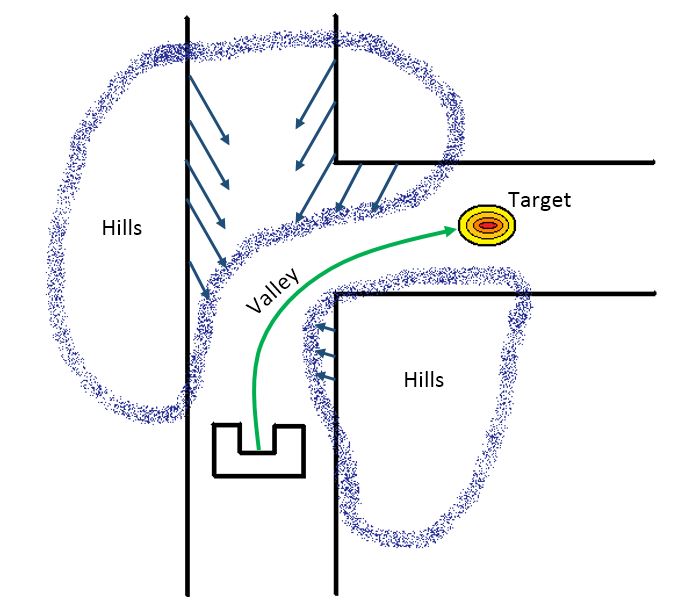
Imagine the top view of the robot in the maze being plotted a 2D (x,y) field. The third dimension is then given by the obstacles in its path or its goal. The obstacles are depicted as hills, where the goal is depicted by a valley. To solve the maze, the robot has to follow the optimal path to the lowest point of that third dimension. The hills represent positive potential, the valleys a negative one. All of the potentials in the circumference of the robot are summarized. This sum is then equal to the total potential. | |||
U(q) = U<sub>att</sub>(q) + U<sub>req</sub>(q) | |||
The attractive or repulsive force of an object is then equal to: | |||
F(q) = -∇U(q) | |||
Where F(q) depicts the change in Potential field. The robot uses the laserdata to get information about the distance to the walls. It then identifies, using a function, what direction the resultant negative potential vector has. At that moment in time, the robot moves to the specified location and repeats the loop. He follows a gradient descent given by: | |||
c´(t) = -∇U(c(t)) | |||
=== Trajectory === | |||
A potential field was implemented in the real time system and was used in turning around corridors and corners by using data from Find Geometries. When the global state monitor issued a direction to turn depending on the geometric shape | |||
encountered at the junction/corner, the potential fied algorithm was called. It implementation in theory was rather simple. It used the real time laser data to locate a suitable point in the turning direction which we defined after careful calibration. The point obtained is then associated with an attractive field while the non desirable locations in the map are given a repulsive field. | |||
An example, if the following geometric shape was encountered, the global monitor will issue the right state command to be implemented. This information is then passed to the turn function which will call the potential field function. The diagram below shows the way the robot sees the map after the potential fields have been implemented. | |||
[[File:Potential Field Navigation.JPG|frameless|center|upright=3.5|Environment detection: T-junction]] | |||
The move forward algorithm was implemented when the global state monitor called the move forward state. The algorithm acomplished three feats. Position alignment, Angular alignment and drive forward. This was implemented in a relatively simple manner. While the robot is moving, the algorithm is constantly scanning and checking if the position and angle of the robot are at the "0 mean" position and angle. Each time a deviation from the mean position is noticed, the error is obtained by subtracting the respective positions to obtain the error of the position or angle. A Potential-Differential controller is then used to eliminate the error and correct the robots position. | |||
== Analysis of the Competition == | |||
==== First Run ==== | |||
During the first run PICO exited from its starting position, before proceeding to take the first right turn and attempting to solve the maze. The robot continued through, taking a second right turn, but was unable to make the left turn towards the door due to moving too fast and detecting the turn to the right as being the optimal path. This led to PICO performing a continuous loop around the starting block. After 3 attempts to make the door, the run was aborted. | |||
==== Second Run ==== | |||
This time PICO was positioned in the doorway with the door open. Upon starting, it proceeded to exit the hallway and enter the open space. When this occurred the robot took measures to keep one wall within its view, travelling along the right hand wall throughout the open space. At the end of the space was the exit of the maze, which PICO managed to navigate through successfully. | |||
==== Overall Notes ==== | |||
Both trials were very smooth, turning corners without hesitation. Secondly, the robot did not collide with any obstacles in the maze (walls or door). One downside was an inability of the robot to navigate the smaller sections, such as dead-ends and the door, which can be attributed to the thresholds selected in the code. | |||
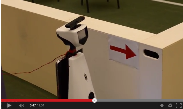
Below is the video of our first attempt to complete the maze. | |||
[[File:Video.png|center|250px|link=https://www.youtube.com/watch?v=_IoCZJR9M-Q&feature=youtu.be]] | |||
= Conclusions and Recommendations = | |||
== Conclusions == | |||
We were able to finish the maze by changing the initial position of the PICO, which has a | |||
* Modular design | |||
* Finite state machine which makes it easy to add additional states | |||
* Super smooth cornering by using Potential Fields. | |||
* Able to detect edges and geometries while the robot is moving. | |||
* Collision detection and step back | |||
We could not finalize some of our targets such as; | |||
* Able to localize the robot in a dynamic environment using Kalman filter. | |||
* Able to behave properly in an open space (it stuck in loop sometimes) | |||
* Maze tree is constructed but couldnt used efficiently. | |||
== Recommendations == | |||
Possible improvements for a faster maze solving PICO are: | |||
* System architecture should be defined well, by showing all decoupled functions and their interaction. Since this project is a team, in this way we could work on different parts on the code. | |||
* Odometry data is not trustable for the turning. | |||
* Depth-First Search algorithm can give efficient results with a proper maze tree. So in this way PICO will also be able to solve a more complex maze, including loops. | |||
* Mapping is hard and time consuming. If it can be implemented well, it can be useful but maze can still be finished by the robot without localizing it. | |||
* For this challange there is no need for a complex code. We tried to keep it simple as possible. | |||
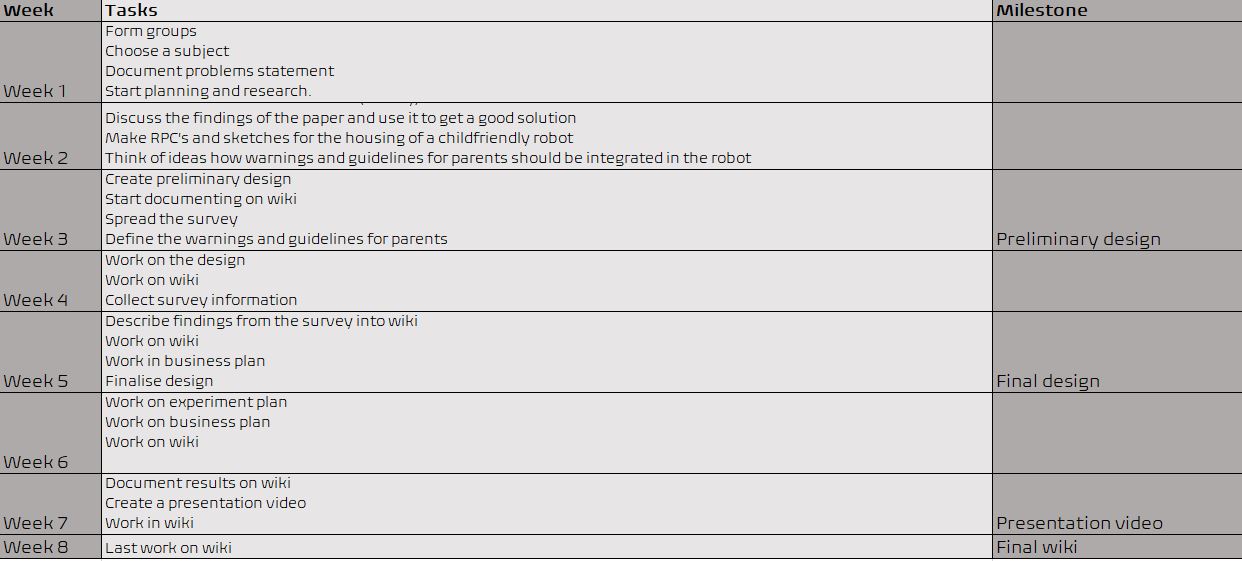
= Time Survey Table 4K450 = | |||
[[File:Planning.JPG|center]] | |||
=== Total Score(Based on total working hours): === | |||
*Ugo : 10 | |||
*Cagil : 9.7757 | |||
*Akash : 9.6412 | |||
*Angus : 9.4394 | |||
*Floris: 9.4394 | |||
*Ashish: 9.3273 | |||
Latest revision as of 23:51, 26 June 2015
Group Members
| Name: | Student id: | E-mail: |
| Akash Agarwal | 0923269 | a.agarwal@student.tue.nl |
| Angus Pere | 0926353 | a.f.pere@student.tue.nl |
| Ashish Yadav | 0925559 | a.yadav@student.tue.nl |
| Floris Remmen | 0920072 | f.remmen@student.tue.nl |
| S. Cagil Mayda | 0926975 | s.c.mayda@student.tue.nl |
| Ugonna Mbaekube | 0927006 | u.o.mbaekube@student.tue.nl |
| René van de Molengraft | Tutor | m.j.g.v.d.molengraft@tue.nl |
Initial Design
Goal
The goal of the “A-Maze-ing challenge” is to design and implement a software for the PICO robot to navigate through a maze autonomously while optimizing time.
Requirements
To program a PICO robot to participate in the “A-Maze-ing challenge”, it is desired that the software meets the following requirements.
- The PICO robot should be able to navigate through any maze autonomously regardless of its configuration. (Autonomous Behaviour)
- The PICO robot should be able to avoid all obstacles during its navigation through the maze including contact with the walls of the maze.(Collision Avoidance)
- The PICO robot should never get “stuck” at any position in the maze and should make desired movements.(Movement)
- The PICO robot should be able to make use of its sensors to navigate the maze.(Use of Sensors)
- The PICO robot should have some sort of “memory” that prevents it from moving back towards paths already navigated through.(Awareness of the environment)
- The PICO robot should be able to find the optimal path through the maze while optimizing time.(Optimal Path Calculation)
- After navigating through the maze, the PICO robot should be able to autonomously terminate its movement.(Termination)
Functions
The basic functionality of the robot that are assigned to requirements in order to reach the goal are as follows:
1) Drive
- Move Forward
- Move Backwards (Reverse)
2) Obstacle & Wall Detection
- Calculation of Distance to objects
3) Decision Making
- Turn Left/Turn Right
- Rotate
- Termination of movement on completion of the maze
4) Optimal Path Algorithm
- “Memory” storage
- Localisation
Components and Specificications
Initial Schematic overview of the components to be used in the software design
1) Task Context: Controls the implementation of the robots functions depending on the challenge and environmental context.
- Task Monitor: Monitors the implementation of the robots functions and sends the information to the task control feedback.
- Task Control Feedback: Implements control action on the robot based on information received from the task monitor.
- Task Control Feedforward: Contributes in the implementation of control actions on the robot depending on the state and the goal of the challenge.
2) Environmental Context: Semantic maze model.
3) Challenge Context: All information regarding the rules and the goals of the “A-Maze-ing challenge” are stored in this context.
4) Robot Context: This incorporates the low level specifications of the PICO robot.
5) Skills Context: Contains the above mentioned robot functionalities.
Interfaces
1) Challenge Context – Environmental Context: deals with presumptions about the maze and goal methodology.
2) Skill Context- Robot Context: deals with sending commands to the low-level hardware.
3) Task Context- Environmental Context: provides information to the task context about decisions to be made in the maze.
4) Challenge Context- Task Context: provides the aim of the challenge context to the task context in order for the task context to adhere to the rules of the game while decision making.
5) Task Context – Skill Context: Allocates the necessary skill dependent on the contribution of the task control feedforward and feedback.
Corridor Competition
For this competition, it was aimed to exit the corridor succesfully with an easy approach.
Hardware Components
- Wheels:
- The robot doesnt move in a straight line when a move command is given in the x direction. This is because of the omniwheels which make the robot rotate whenever it moves forward. For this reason we need an allignment algorithm.
- Laser Data:
- The laser stores position information and angular information in laser data framework
- Every laser needs to be calibrated and multiple lasers are used to get a homogenous result and trustable data.
- Odometry Data:
- Gives information about the relative changes in X, Y and angular position. The first navigation algorithm was based on this odometry data, but since good results were not obtained, it was changed by using laserdata.
Initial Software Design
- Initial Movement: Robot starts with a constant speed and move forward through the corridor.
- Collision Detection: With using the laser data, distance to the wall or any other obstacles (no obstacles in this case) can be determined. If the distance becomes less than 0.1 metre, robot will stop to avoid collision.
- Position Alignment: It is observed that, due to feature of omni wheels, robot sometimes can not go straight. So in the algorithm, Pico is forced to stay in the middle of the corridor by calculating the distance to the right and left wall by using laser data.
- CheckCorridor: Robot will constantly check the distances to the left and right wall. If the distance to one of them exceeds the threshold (max.width has already known) turn left/right command will be executed.
- Turn Left/Right: After robot moves in the middle of the gap, it turns +/-90 degrees by using the odometry data. When it is turned, it again starts moving forward.
- Finish: Since the distance to finish can be approximated, after moving some distance, robot will stop automatically.
States of the initial design can be seen in the following figure:
Features of the Software
Collision Detection
When the distance between the robot and wall becomes smaller than 0.1 meters, initial collision detection function stop the robot before it hits the wall. This function will be upgraded further.
Position Alignment
Pico looks at its environment and takes the information from the laserdata to calculate the distance to the walls. If the difference in distance to both left (P1) and right (P2) side of the wall is the minimum possible, then a perpendicular relation is found. This also means that pico is going in a straight line through the centre of the hallway.
Find the Gap
While moving forward the above condition is checked at every time step, correcting itself where necessary. When pico encounters a turn, one of the distance vectors will increase drastically. At that point, pico stops and looks at its environment. It calculates (in the direction of the increased vector) the shortest possible distance to the wall and saves this point as the rotation point. The other side of the gap is calculated by using the same technique, but in a different quadrant. The rotation radius is then the half of the distance between these two points. After the rotation is complete pico starts from the beginning again.
Tests before corridor competition and Updates to Software
The day before the corridor competition, our algorithm was tested on the robot 3 times. On the first try, the robot solved the maze. On the second try we noticed that although the robot was aligning its position to the centre, the robot's angle was slightly tilted from the "0" mean angle position. This angular tilt of the robot caused the robot to fail to finish the test run on the second and third try.
Final amendment to code before corridor competition: The night prior to the competition we decided to amend the code and include an angular alignment function to eliminate the angular tilt. This code was tested on the simulation and it worked perfectly.
Analysis of the Competition
Corridor Competition: In the corridor competition, we were given 2 tries like every other group. On our first try, the robot did not move. We ran our code but the robot seemed to do nothing. There was no behaviour. On the second try, we asked the coordinator to reset the odometry data which he did and we ran our code. The robot moved roughly for 3 seconds and then stopped.
Software bugs during the corridor competition. We had numerous bugs in our software during the competition. The first bug in our software was the angular alignment function we included the previous night. Due to haste, we used odometry data and a while loop in the code. The function checked if the odometry angle was at "0" mean. We defined 0 mean as odometry angle between 0.1 and -0.1. Anytime the odometry angle went above these angles while the robot was not turning, we sent the error back as a feedback to a while loop and used the error to determine if we were to align our angle in the x or y direction. This implementation worked on the simulation so we did not realise how infeasible this method was on the real system. The while loop ran at an "infinitely" higher frequency than the robot thus the odometry variables were not updated in real time. The second bug was from using odometry data constantly. Odometry data accumulates error overtime and returns very erroneous data which causes erratic behaviour.
Reason for robot behaviour in first try: The odometry data accumulated error over time from the previous groups so when we ran our program, the odometry sent erroneous data as feedback thus the condition for the loop to break was never met which caused the robot to do nothing.
Reason for robot behaviour in second try: After the coordinator reset the odometry data, we reran our code. The behaviour was caused by the while loop. After 3 seconds, the angular position moves away from the "0" mean angular position. The software logic moved into the while loop and got stuck in the while loop since the while loop runs "infinitely" faster than 40 Hz which the robot which runs at thus causing the variables never to be updated
After the corridor competition, alignment was added to the code properly. The code can be seen below. Now the alignment has done by using just laser data. By updating the alignment, we were able to finish corridor competition.
void move_forward(bool move_status, global_state_monitor &state)
{
   io.readLaserData(scan);
   double left_dist_to_wall = scan.ranges[893]; //distance at +90 degrees
   double right_dist_to_wall = scan.ranges[107]; //distance at -90 degrees
   double align_diff = left_dist_to_wall-right_dist_to_wall;
   double closest_point_right  = findmin(scan,1);
   double closest_point_left = findmin(scan,2);
   double angle_diff = (closest_point_right - 107)*0.004;
   if((abs(align_diff) < 0.08)  || ( abs(align_diff) > 0.5) ){
           align_diff = 0;
       }
   if((abs(angle_diff) < 0.008) || ( abs(align_diff) > 0.15)){
       angle_diff = 0;
   }
   if(move_status)
    {
        io.sendBaseReference(0.4, align_diff/2, angle_diff/6);
    }
   else
    {
        io.sendBaseReference(0, 0, 0);
    }
}
Maze Competition
Components and Specificications
Initial Schematic overview of the components to be used in the software design
Interfaces
1) Environmental Context - Task Context:
The task context identifies the geometric shape at the junction, and then places a node and saves the node's orientation, parents, and children. The information regarding the node is then passed back to the environmental context which then updates the the local map. Based on the type of junction encountered, the task monitor then sends this information to the skills context
2) Task Context - Skills Context:
The skills context then implements the particular robotic skill needed to traverse the geometric shape encountered. After the required skill is implemented, the information is sent back to the task context which then updates the task monitor. The task monitor then sends the information to the environmental context which updates the position of the robot in the maze.
3) Skills Context - Robot Context:
Dependent on the skills to be implemented, the code is sent to the low level robot context which then implements the particular behaviour wanted and passes the information back to the skills context
4) Finite State Machine:
In order to navigate within the maze, a finite state machine (FSM) was implemented. The purpose of the FSM was to assign the right state which is dependent on the occurence of an event or multiple events. Below is the state diagram showing the transition between states.
From the diagram, it can be seen which respective event triggers a state.
The events are
- if right corner detected
- if deadend detected
- if door present
- if door absent
- has turned around
- if right corner present
- if left corner present
- has turned
- if multiple exit junction detected
Building our local Map
In this assignment, we thought about building a world map using the hector mapping library but encountered several issues with the importing. on further thought we decided to use a local map which will be built as we navigate through the maze. At the starting position of the maze we place a node with index 1 and store its orientation. On moving, when a junction (junction here meaning a geometric shape which would require the robot to change state) is encountered, another node is placed there storing its orientation, parent and children. Depending on the type of junction encountered, the second node will check the left, right and forward extreme of the junction and then store these positions as its children in the map. This process is continued till the entire map has been stored.
Algorithm
The algorithm we have adopted is a subset of the depth first search algorithm with the nodes placed at respective junctions. Each node comprises of a parent and several children.The children of the nodes are at the left and right extremes of the junction. When the robot moves down a desired path and encounters a dead end, the robot is then able to backtrack to the previous junction by moving to its parent. When a node is visited, this information is stored and used when searching for unexplored areas. This technique is not optimal as it focusses on navigating through the entire maze rather than searching for the optimal distance but it is more reliable as it makes sure it explores the entire span of the maze. Also anytime a node is visited, the index of the node is stored in the visited section thus enabling us to know when a node has been visited and thus enabling us to navigate through the maze without entering an infinite loop.
Depth First Search
This algorithm is utilized for traversing tree/graph data structures. Starting at a root position, the algorithm moves through the tree along each possible branch before back-tracking. Although it is not considered the most efficient method for maze solving (unlike A*), for our intentions it is a more comprehensive system when compared other solving-algorithms. The image below shows a simple data structure that can be tackled with DFS. Starting at node 1, the algorithm then moves to 2, 3, and then 4, at which point it reaches the end of a branch. When this occurs the algorithm moves back to the previous node (in this case 3), and then attempts to take another branch (to node 5). This system continues throughout until the entire branch is mapped.
When compared with a simple algorithm such as the “wall-follower” method (WFM), which follows either the left- or right-wall (depending on specifications in the code) to solve the maze, DFS can be considered more robust overall. This comes down to 2 factors: firstly, the WFM is considered one of the slowest methods (heavily dependent on the size of the maze and starting position); and secondly, the WFM is susceptible to entering a loop within the maze which it cannot exit. DFS on the other hand can be considered a slow method, but it is very unlikely to get caught in a loop due to the formation and tracking of nodes within the algorithm, as mentioned above.The gif below shows how DFS is utilised by PICO to solve the maze.
Top Level Decision
This is the "brain" in the robotic software. It issues commands in the software. Our algorithm to solve the maze focused on building a maze tree obtained by the geometric shapes in the local map (corners, deadends, etc), such as in the gif above. The global state monitor (GSM) made sure our algorithm was strictly adhered to. The monitors aim was for the robot to navigate through all the nodes until the exit is found.
How the "Brain" works
When the robot starts the system is initiated. After initialisation the GSM calls the "move forward" function. The state remains in "move forward" until the robot comes across a geometric junction. The GSM then calls the "detect geometric shape" function to identify which shape has been encountered. Depending on the determined shape, a specific event is triggered. When the event is triggered the GSM changes the state of the final state machine.
Event
If a right corner is detected → By our definition of right turn, only one possible movement is possible, which is the "right turn" geometry. The GSM then changes the state to "right turn".
If a left corner is detected → The same occurs as in the right turn, with the state being changed to "left turn" instead.
If deadend → The state is changed to check for door. If a door is found (waiting for 5 seconds and detecting an exit), the state is changed to "beep and move forward". If no door is present, the state is changed to "turn around".
If a multiple junction exit is detected → Depending on the information from the maze tree, the GSM calls the state which turns according to the information.
Code Interaction
The main program uses some defined robot functionalities in order to achieve its goal. Below, interaction of all functions and global ros input variables can be seen.
Find Geometries
The robot should be able to recognize all possible geometries in order to navigate through the maze. State changes will be determined by detected geometries while the robot is moving. Defined geometries are shown belown:
Main Algorithm:
- Start scanning the environment from -90 to 90 degrees with respect to the robot. Pico's view is separated as left, middle and right. Middle view is responsible for measuring the distance in front of Pico. Therefore this distance is calculated by using range of points inside the middle view in order to get more reliable result. Left and right views are responsible for the detection of edges in front of the Pico. Views can be seen at the figure below:
- First edges of the geometries are found by comparing all consecutive elements in the left and right views.
- All points [i] in the separated views are compared with next two consecutive beams. At the figure left below, the red dashed line will be compared with next laser data in terms of distance and since the difference in distance between first point and next points is higher than the threshold, this point will be accepted as edge.
- For the corridors, there will be a second edge. This can be found by continue scanning left/right views starting from the angle of the first edge. In this range, the smallest point to the robot will be our second edge. Threshold is given for the distance between these points. If the distance between first edge and second is smaller than this threshold, that means the found geometry is just a hole. Otherwise, the edges are saved as an element for the corridors. At the figure right below, new view is defined as yellow area, and the most closest point to the robot in that area is accepted as second edge.
- Found edges can be seen at figure belown. If l1 and l2 edges are found that means the robot is encountered with left corridor, if r1 and r2 edges are found that means the robot is encountered with right corridor and if both l1, l2, r1 and r2 edges are found that means the robot is encountered with 4-way junction.
- For the corners, there won't be a second edge. If the first edge is found and the front distance (that is calculated before by using middle view) is lower than the defied threshold, that means the found edge belongs to a left/right corner. If C1,L1 and R1 is found that means that the robot is encountered with t-junction. C1 is saved as point when the calculated distance of the robot front view is lower than the threshold. In that way we can detect whether the detected shape is corridor or corner.
The following is the code for the left corridor check.
 void LeftCorridorCheck(point (&left_cor)[2], global_state_monitor &state,geometric_shapes &shapes,double &left_corridor_exist){
   io.readLaserData(scan);
   double min=1000;
   double index_second_corner=0;
   double index_first_corner=0;
   for(unsigned int i = 893; i > 650;i--){
     if( abs(scan.ranges[i-1]-scan.ranges[i] && abs(scan.ranges[i-2]-scan.ranges[i]) > 0.1){ // finds the first edge by comparing near points
         //cout << "corridor is detected on the left. first phase "  << i << endl;
         index_first_corner = i;
         break;
         }
    }
   if(index_first_corner > 0){ // if the first edge is found, then look for a second edge and find it.
       for(unsigned int j = index_first_corner-1; j > 510;j--){
                    if((abs(scan.ranges[j]) < min) && (scan.ranges[j] > 0.1)){
                                    min = scan.ranges[j];
                                    index_second_corner = j;
                                }
                }
       if(abs(index_first_corner - index_second_corner) > 40){ // if the index between the edges smaller than 40, it means that is gap otherwise it will be saved as left corridor
                     left_cor[1].angle = index_first_corner;
                     left_cor[1].distance = scan.ranges[index_first_corner];
                     left_cor[2].angle = index_second_corner;
                     left_cor[2].distance = scan.ranges[index_second_corner];
                     shapes.T_crossing_left_straight = true;
                     left_corridor_exist = true;
                 }
       else{
           left_cor[1].angle = 0;
           left_cor[1].distance = 0;
           left_cor[2].angle = 0;
           left_cor[2].distance = 0;
       }
   }
}
Special Case: DeadEnd
The deadend occurs when no edges are found and the front of the robot is blocked (smaller than specified threshold). Then the robot waits for 5 seconds and again checks the distance to determine if it is still a deadend or if it has become an exit. If it is an exit, PICO continues moving forward. If it is a deadend the robot then turns 180o.
Movement
The move forward algorithm was implemented when the global state monitor called the move forward state. The algorithm acomplished three feats. Position alignment, Angular alignment and drive forward. This was implemented in a relatively simple manner. While the robot is moving, the algorithm is constantly scanning and checking if the position and angle of the robot are at the "0 mean" position and angle. Each time a deviation from the mean position is noticed, the error is obtained by subtracting the respective positions to obtain the error of the position or angle. A Potential-Differential controller is then used to eliminate the error and correct the robots position. The left gif shows what happens when PICO starts in the specified starting position, as in the first run. The right gif shows the second run of PICO, starting in the door corridor (with door open).
Path Planning Method - Potential Field
This methodology is used to increase the quality of navigation throughout the maze. Imagine the top view of the robot in the maze being plotted a 2D (x,y) field. The third dimension is then given by the obstacles in its path or its goal. The obstacles are depicted as hills, where the goal is depicted by a valley. To solve the maze, the robot has to follow the optimal path to the lowest point of that third dimension. The hills represent positive potential, the valleys a negative one. All of the potentials in the circumference of the robot are summarized. This sum is then equal to the total potential.
U(q) = Uatt(q) + Ureq(q)
The attractive or repulsive force of an object is then equal to:
F(q) = -∇U(q)
Where F(q) depicts the change in Potential field. The robot uses the laserdata to get information about the distance to the walls. It then identifies, using a function, what direction the resultant negative potential vector has. At that moment in time, the robot moves to the specified location and repeats the loop. He follows a gradient descent given by:
c´(t) = -∇U(c(t))
Trajectory
A potential field was implemented in the real time system and was used in turning around corridors and corners by using data from Find Geometries. When the global state monitor issued a direction to turn depending on the geometric shape encountered at the junction/corner, the potential fied algorithm was called. It implementation in theory was rather simple. It used the real time laser data to locate a suitable point in the turning direction which we defined after careful calibration. The point obtained is then associated with an attractive field while the non desirable locations in the map are given a repulsive field.
An example, if the following geometric shape was encountered, the global monitor will issue the right state command to be implemented. This information is then passed to the turn function which will call the potential field function. The diagram below shows the way the robot sees the map after the potential fields have been implemented.
The move forward algorithm was implemented when the global state monitor called the move forward state. The algorithm acomplished three feats. Position alignment, Angular alignment and drive forward. This was implemented in a relatively simple manner. While the robot is moving, the algorithm is constantly scanning and checking if the position and angle of the robot are at the "0 mean" position and angle. Each time a deviation from the mean position is noticed, the error is obtained by subtracting the respective positions to obtain the error of the position or angle. A Potential-Differential controller is then used to eliminate the error and correct the robots position.
Analysis of the Competition
First Run
During the first run PICO exited from its starting position, before proceeding to take the first right turn and attempting to solve the maze. The robot continued through, taking a second right turn, but was unable to make the left turn towards the door due to moving too fast and detecting the turn to the right as being the optimal path. This led to PICO performing a continuous loop around the starting block. After 3 attempts to make the door, the run was aborted.
Second Run
This time PICO was positioned in the doorway with the door open. Upon starting, it proceeded to exit the hallway and enter the open space. When this occurred the robot took measures to keep one wall within its view, travelling along the right hand wall throughout the open space. At the end of the space was the exit of the maze, which PICO managed to navigate through successfully.
Overall Notes
Both trials were very smooth, turning corners without hesitation. Secondly, the robot did not collide with any obstacles in the maze (walls or door). One downside was an inability of the robot to navigate the smaller sections, such as dead-ends and the door, which can be attributed to the thresholds selected in the code.
Below is the video of our first attempt to complete the maze.
Conclusions and Recommendations
Conclusions
We were able to finish the maze by changing the initial position of the PICO, which has a
- Modular design
- Finite state machine which makes it easy to add additional states
- Super smooth cornering by using Potential Fields.
- Able to detect edges and geometries while the robot is moving.
- Collision detection and step back
We could not finalize some of our targets such as;
- Able to localize the robot in a dynamic environment using Kalman filter.
- Able to behave properly in an open space (it stuck in loop sometimes)
- Maze tree is constructed but couldnt used efficiently.
Recommendations
Possible improvements for a faster maze solving PICO are:
- System architecture should be defined well, by showing all decoupled functions and their interaction. Since this project is a team, in this way we could work on different parts on the code.
- Odometry data is not trustable for the turning.
- Depth-First Search algorithm can give efficient results with a proper maze tree. So in this way PICO will also be able to solve a more complex maze, including loops.
- Mapping is hard and time consuming. If it can be implemented well, it can be useful but maze can still be finished by the robot without localizing it.
- For this challange there is no need for a complex code. We tried to keep it simple as possible.
Time Survey Table 4K450
Total Score(Based on total working hours):
- Ugo : 10
- Cagil : 9.7757
- Akash : 9.6412
- Angus : 9.4394
- Floris: 9.4394
- Ashish: 9.3273
