Embedded Motion Control 2015 Group 8: Difference between revisions
No edit summary |
|||
| (114 intermediate revisions by 7 users not shown) | |||
| Line 4: | Line 4: | ||
<td width="150px"><b>Name:</b></td> | <td width="150px"><b>Name:</b></td> | ||
<td width="120px"><b>Student id:</b></td> | <td width="120px"><b>Student id:</b></td> | ||
< | <td width="120px"><b>E-mail:</b></td> | ||
< | |||
</tr> | </tr> | ||
<tr> | <tr> | ||
<td>Ruud Lensvelt</td> | <td>Ruud Lensvelt</td> | ||
<td>0653197</td> | <td>0653197</td> | ||
<td>g.lensvelt@student.tue.nl</td> | |||
</tr> | </tr> | ||
<tr> | <tr> | ||
<td>Stijn Rutten</td> | <td>Stijn Rutten</td> | ||
<td>0773617</td> | <td>0773617</td> | ||
<tr> | <td>s.j.a.rutten@student.tue.nl</td> | ||
</tr> | |||
<tr> | <tr> | ||
<td>Bas van Eekelen</td> | <td>Bas van Eekelen</td> | ||
<td>0740175</td> | <td>0740175</td> | ||
<tr> | <td>b.v.eekelen@student.tue.nl</td> | ||
</tr> | |||
<tr> | <tr> | ||
<td>Nick Hoogerwerf</td> | <td>Nick Hoogerwerf</td> | ||
<td>0734333</td> | <td>0734333</td> | ||
<tr> | <td>n.c.h.hoogerwerf@student.tue.nl</td> | ||
</tr> | |||
<tr> | <tr> | ||
<td>Wouter Houtman</td> | <td>Wouter Houtman</td> | ||
<td>0717791</td> | <td>0717791</td> | ||
<td>w.houtman@student.tue.nl</td> | |||
</tr> | |||
<tr> | |||
<td>Vincent Looijen</td> | |||
<td>0770432</td> | |||
<td>v.a.looijen@student.tue.nl</td> | |||
</tr> | |||
<tr> | <tr> | ||
<td>Jorrit Smit</td> | |||
<td> | <td>0617062</td> | ||
<td> | <td>j.smit@student.tue.nl</td> | ||
</tr> | |||
<tr> | |||
<td>''René van de Molengraft''</td> | |||
<td>''Tutor''</td> | |||
<td>''m.j.g.v.d.molengraft@tue.nl''</td> | |||
</tr> | </tr> | ||
</table> | </table> | ||
| Line 37: | Line 50: | ||
<!-- White space --> | <!-- White space --> | ||
= | = Design = | ||
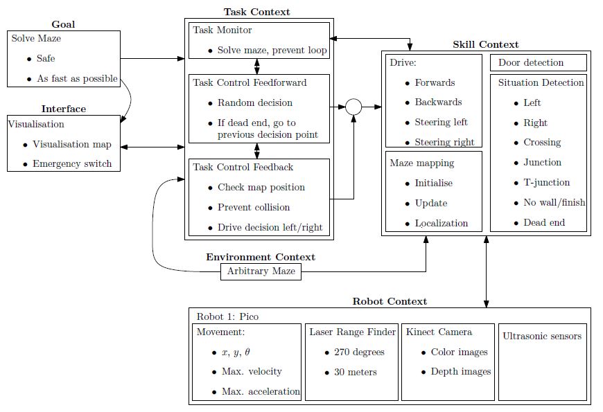
As a start of the course the initial design of the software is discussed. The design is divided into several parts, the general flow chart for the software design is shown in Figure 1.1. In the upcoming sections the initial design will be described. | As a start of the course the initial design of the software is discussed. The design is divided into several parts, the general flow chart for the software design is shown in Figure 1.1. In the upcoming sections the initial design will be described. | ||
| Line 133: | Line 146: | ||
To prevent unwanted behavior of the robot due to bugs in the software, a kill switch should be implemented in the interface such that the robot can remotely be switched off. | To prevent unwanted behavior of the robot due to bugs in the software, a kill switch should be implemented in the interface such that the robot can remotely be switched off. | ||
= Initial software for corridor competition = | |||
In the initial design of the software the general framework of functions provided in Figure 1.1 is translated into a composition pattern to solve the corridor challange. The initial software consists of the skill context and task context. The skill context can be divided into two skills, the 'Drive in maze' and 'Feature detection'. The 'Drive in maze' ensures that PICO can move between the walls in the direction of a given setpoint. The 'Feature detection' detects openings in the maze, like junctions. The 'Task control' get information about the features and determines a setpoint for the 'Drive in maze' function. This software is used to complete the corridor challenge. | |||
== Drive in maze == | |||
=== Potential Field Method === | |||
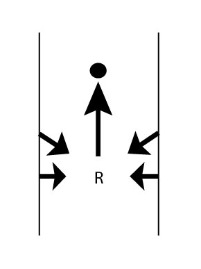
The Potential Field Method is used to drive in a corridor. When the setpoint is determined, PICO needs to drive towards it without hitting any wall. With the Potential Field Method virtual repulsive forces are applied to PICO for every laser point. The force caused by a point depends on the distance between PICO and a laser point. The virtual force is defined as F = -1/(r^5), where F is the resulting force and r is the distance between PICO and the laser point. The force is pointing away from the obstacle. When the sum is taken over all repulsive forces, the net repulsive force is pointing away from close obstacles. | |||
The setpoint is added as attractive force, which results that PICO drives in the direction of the setpoint without hitting the wall. | |||
This Potential Field Method is also used as safety, because the repulsive forces ensure that PICO does not drive into a wall. The Potential Field Method is illustrated in Figure 2.1. | |||
<gallery perrow="1"> | |||
File:potential_field.jpg|Figure 2.1: Potential Field Method in corridor. | |||
</gallery> | |||
=== Drive Function Block === | |||
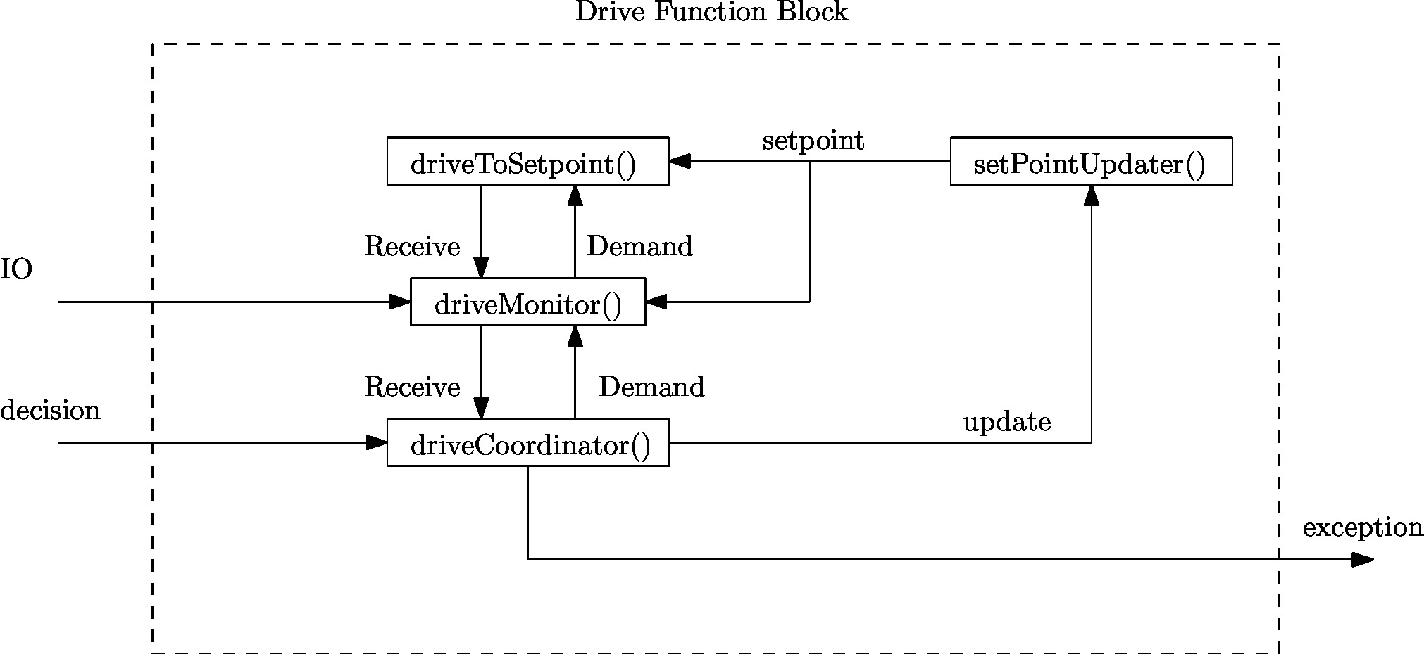
[[File:Drive Function Block.jpg|400px|thumb|right|Figure 2.2: Composition pattern of the general Drive Function Block software on PICO.]] | |||
Since the required action on a junction is either one of three cases, i.e. drive straight, left or right, a general drive function blocks has been implemented who’s framework can be reused for other functions. Thus though the function of a drive function block may vary depending on its goal, their overall composition is similar as the composition pattern provided in Figure 2.2. In Figure 2.2 the composition pattern is shown for a general drive function block and communication to its environment is provided through:<br> | |||
* ''Robot data'' provides the data the robot measures through its LRF and odometry sensors. <br> | |||
* ''Decision'' provides the decision from the ''Coordinators()''. <br> | |||
* ''Exception'' allows the drive function block to communicate to the main loop if an exceptional case occured. <br> | |||
Depending on the decision variable provided a drive function block either turns on or stays off. When a drive function block finishes its task it changes the parameter in ''Decision'' to the drive straight block or if it finds a condition which is outside its task description it sends an exception through the Exception variable. The general drive function block consists of four distinct parts: | |||
* ''driveCoordinator()'' verifies whether the current situation corresponds to the required action in the decision variable, i.e. when driving straight only a straight corridor is detected, otherwise it communicates to the globalMonitor() through the exception variable. The coordinator is always vigilant on a potential command from the globalCoordinator(). <br> | |||
* setPointUpdater() adjusts the global setpoint to compensate for the robots travelled distance the setpoint. For a detailed explanation see the next section. <br> | |||
* driveToSetpoint() implements the actual motion towards a setpoint using the potential field, while constantly detecting changes in the robots environment. <br> | |||
* driveMonitor() receives data from the setPointUpdater() and driveToSetpoint() and determines the robots current location, orientation and compares what the robot actually sees against the previously provided setpoint. <br> | |||
In case a turn function block is used there are extra functionalities used in the drive function block. Which are defined as | |||
* ''setPathPlan()'' determines intermediate setpoints towards the goal setpoint to guarantee the robot turns 90 degrees into a corner. This function is only called once at the start of a turn and sets a list containing all intermediate setpoints. | |||
* ''driveConfigurator()'' selects a setpoint from the list if has not been marked as already reached by the ''driveTurnCoordinator()''. | |||
More information on the actual implementation can be found below. | |||
== Feature detection == | |||
[http://cstwiki.wtb.tue.nl/index.php?title=Embedded_Motion_Control_2015_Group_8#Feature_detection_2 See Feature_detection] | |||
== Task control == | |||
In default mode the robot drives straight and while in this straight mode the hough detect returns setpoints for a corridor left, straight and right (see below). If no opening is detected from the hough detect functions the setpoint returned equals zero. The ''driveStraightMonitor()'' monitors these setpoints while in drive straight mode and has three distinct states; | |||
* No setpoint is detected either left or right. In which case the monitor does not alter the state of the ''driveStraightCoordinator()'' by sending a message that nothing changed with respect to the default mode. | |||
* A setpoint is detected either left or right, but it is not within range. In this case the monitor again does not alter the state of the coordinator by not sending a message. | |||
* A setpoint is detected either left or right. In this case the monitor sends a message to the coordinator which make a decision based on all provided data from the monitor. | |||
=== Drive functionality === | |||
[[File:EMC2015_group8_Exploination_corrections_drive_Straight.jpg|200px|thumb|right|Figure 2.3: Situation when the robot is driving straight, but not aligned with the walls.]] | |||
==== Setpoint when Driving straight ==== | |||
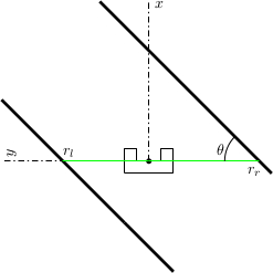
When the robot needs to drive straight, its setpoint is initially set to the front. However, Pico will not be perfectly aligned with the walls on both sides and will not perfectly drive in the middle of those walls. To keep the right orientation and to keep the robot in the middle of the corridor throughout the challenge,the setpoint needs to be be updated. In Figure 2.3, the situation is shown when the robot is not aligned. The orientation of the robot is shown in cartesian coordinates. Under the assumption that the walls are straight, the position and orientation of these walls can be estimated with a first order polynomial approximation. This approximation is obtained using a least squares method using 20 datapoints on each side. For both sides, the distance <math>r_l</math> to the wall on the left side and the distance <math>r_r</math> to the right are determined, as well as the orientation <math>\theta</math>. Now, the setpoint can be updated in y-direction using these data and some basic geometric knowledge. To make the system more robust against noise, the data are averaged over the last 10 iterations. This results however in a system which reacts slower to changes in the environment. In combination with the driving function that was used, some tests showed there was too much overshoot resulting in an unstable system. Therefore, the amount of correction in <math>y</math>-direction was scaled with a gain with an absolute value between 0 and 1. | |||
==== Setpoint when Driving a corner ==== | |||
[[File:Corridor start.jpg|250x250px|thumb|right|Figure 2.4: Starting step in driving to a setpoint in a turn.]] | |||
By default the robot assumes it’s in a straight corridor and upon reaching a junction the robot switches from the drive function block to a turn block. Before the turn can be made its state is logged, which act as a global marker for the starting point of the robot. The following data is logged | |||
* Odometry data to correct the location of the setpoint with respect to the robot. | |||
* <math>x</math> and <math>y</math> location of the middle of the selected opening. | |||
With this data known the robot calculates intermediate setpoint along an elipsoid using a ''setPathPlan()'' function, to guarantee the robot always finishes a corner with its <math>x</math> axis point straight into a opening. After this initialisation the ''setpointConfigurator()'' is called in the function block to select the previously determined setpoint path sequentially. Since these setpoints are absolute with respect to the corner (they do not vary after starting a turn) the ''setpointUpdater()'' is run to update the current location of the setpoint with respect to the robot. The ''driveTurnMonitor()'' then monitors the current location based on odometry data and the currently selected setpoint from the setpointpath and returns all changed data upon reaching the setpoint to within a certain tolerance. If the setpoint is reached the ''driveTurnCoordinator()'' marks the setpoint in the list of setpoints as reached such that the ''setpointConfigurator()'' knows to select the next setpoint from the list. The code for the turn then corresponds to | |||
* ''turnInitialize()'' | |||
* ''setPathPlan()'' | |||
* ''setpointConfigurator()'' | |||
* ''setpointUpdater()'' | |||
* ''driveTurnMonitor()'' | |||
* ''driveTurnCoordinator()'' | |||
The fashion in which the setpoint is updated with respect to the robot in the ''setpointUpdater()'' is described next. The initial starting point of a turn, i.e. in which data is logged, is shown in Figure 2.4. <br> | |||
Since the robot’s coordinate frame is relative, the previously determined global marker is used to determine the travelled distance and the robot’s orientation. With this data the global setpoint is translated to the robot’s relative frame according to <br> | |||
<math>r_2=r_1-dr,</math><br> | |||
<math>\theta_2=\theta_1-d\theta.</math><br> | |||
[[File:Corridor Turn.jpg|300x300px|thumb|right|Figure 2.5: Intermediate step in driving to a setpoint in a turn.]] | |||
The effect of this update is that the setpoint varies in position when observing it from the robot while it stays at the same location with respect to the absolute marker. An intermediate step in driving through a corner can be seen in Figure 2.4. | |||
Since the robot needs to end up in a corridor with its <math>x</math>-axis aligned with the corridor it is entering both <math>x</math> and <math>y</math> coordinates are required to be met to within a certain tolerance <math>tol</math>, i.e. <br> | |||
<math>y-\Delta S_y< tol.</math> <br> | |||
<math>x-\Delta S_x< tol.</math> <br> | |||
Upon completion of a turn the robot jumps back to driving in its default mode and using the above it is guaranteed that the robot crosses the line in Figure 2.5 upon exiting the turn. Since the odometry data is marked global the axis to determine this <math>\Delta S</math> changes as the robot takes multiple turns to the left or right. In order to take this into account a counter for the amount of left and right turns is set every time a corner is successfully finished and the difference between which determines which axis of the odemetry data is either <math>x</math> or <math>y</math>. | |||
= Evaluating corridor challenge = | |||
PICO managed to finish the corridor challenge. With a time of 21 seconds, we finished at the fourth place. The potential field ensures that PICO did not bump into walls, the corner of the exit was detected and PICO take this corner. However, PICO did not take the corner in a smooth way, because the setpoint in the exit was not at a fixed place. This error is solved after the competition. | |||
Further improvements: | |||
* The function setPointUpdater needs to be updated with LRF data. In the old version the odometry data was used. | |||
* During the corridor competition a fixed gain was used to increase the length of the resulting force of the potential field. This gains needs to be replaced by a function that is dependent on the width of the corridor. | |||
= Software for maze challenge = | |||
== Feature detection == | |||
[[File:R_theta_line.GIF|300px|thumb|right|Figure 2.6: Polar representation of line.]] | |||
To safely navigate through the maze, the robot must be aware of its surroundings. While during the corridor challenge we only used the rough laser data to determine distances en detect openings, we started to develop a new technique for the maze challenge. This technique makes use of the Hough transform, available in the OpenCV-libary. The Hough transform is a technique to determine lines through noisy data, which is generated by our sensors. With this technique, the robot is able to determine all the walls as lines instead in points. This makes it a lot easier and robuster to determine openings in corridors, junctions and turns. | |||
To achieve the best result in real time the LRF data was filtered with a gaussian blur, to apply noise reduction. After that duplicate lines were filtered. This gave a robust way of determining the walls around the robot. | |||
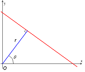
To determine openings in a robust way, the lines are represented by a polar coordinate system, depicted in figure 2.6. In this figure, r is the shortest distance from the origin (which is at the robot) to that line, and <math>\theta</math> the angle that line makes with the robot. If the lines are represented in this way, it become easy to compare different lines with each other and independent of the orientation of the robot. | |||
When simply driving in a corridor the robot detects two parralel lines, one to the right and one to the left. If for instance a T-junction is considered like the one below, the robot sees two parallel lines and one line perpendicular to those two that is not directly connected to the two parallel lines. If this situation arises, the robot immediately knows what kind of crossing it has to deal with. The same holds for the other possible junctions. The turn detection relies on the fact that the one of the parralel lines that the robot sees is suddenly connected with a line perpendicular to it. This means that the opening is at the other side. The image below also depicts a corridor with an opening. If the robot has detect two parallel lines but one has an interruption, it knows it has to deal with an opening. The same holds for a complete crossing with four roads, it just has to detect an extra interruption to the right. At last The dead-end detection is very similar to the first T-junction detection. The robot sees two parallel lines and one perpendicular to it. The only difference is that all lines must be connected for it to be an dead-end. | |||
[[File:Featuresdetection.jpg|800px|center]] | |||
== Door handling/detection == | |||
In feature detection dead ends will be detected, each dead end could be a possible door. The dead end detection places a setpoint just before the possible door, the robot drives to this setpoint. This setpoint is located such that the robot will be in the door area. When the setpoint is reached all velocities are set to zero and the door request is executed. Five seconds after this request feature detection is used to check if a possible door has opened. If this is the case the robot will drive straight through the corridor. If no door has opened, the robot will turn 180 degrees, the history will be updated and the Tremaux algorithm decides what the next action will be. | |||
== Maze mapping/strategy == | |||
==== Determine orientation of the robot ==== | |||
Since the maze is constructed out of corners of 90 degrees, an integer multiple of this value is used to determine the orientation of the robot. The initial orientation is zero degrees, hence the decision at every subsequent junction is added to the initial orientation value. A counter clockwise structure has been applied, resulting in +90 degrees for a left turn, +180 degrees for going back the same path as the driving direction, +270 degrees of a right turn and +0 degrees for straight ahead driving over the junction. When the orientation value is larger or equal to 360 degrees, 360 degrees is subtracted. By keeping track of the orientation at every corner and junction, the orientation relative to the initial orientation is known at all times. | |||
==== Determine orientation number ==== | |||
By driving through the maze, changes are detected based on measured data by the developed detection software. The detection software also communicates what type of situation is detected, for example a T-junction. However, the situation is communicated relative to the current driving direction, so for example if the detection software outputs a T-junction with left en right possibilities, it is possible that it actually is a T-junction in north and south direction. This situation is depicted in Figure 2.5. To obtain usable data for the maze history, the information from the detection software is corrected with a correction number, which basically shifts the information a given amount of places. The number of shifts is determined by the current orientation: 1 for a current orientation of +90 degrees, 2 for a current orientation of +180 degrees, 3 for a current orientation of +270 degrees and 0 for a current orientation of 0 (or 360) degrees. Now all the junctions can be mapped in global wind direction names: North, East, South and West. | |||
[[File:correction_number.png|164x188px|thumb|right|Figure 2.5: Conflict in orientation demonstrated.]] | |||
==== Maze history ==== | |||
The maze history is a vector of classes. Each entry of the vector belongs to a node ID number. Because of the work done in the orientation determination functions above, the maze history function is a matter of bookkeeping and initialization. When the program is started, the straight ahead direction is set to North which is now the global North for the entire maze. Mapping the maze all starts with a detected change in the maze from detection software, which triggers the following actions: | |||
* Only when the <math>1^{st}</math> node is detected: Initialize first node by setting the south exploration value of the <math>1^{st}</math> junction to explored. This implies that the initial driving direction is from south to north, regardless of the ´real´ direction. | |||
* A node is added to the history vector by the push_back functionality for each detected change in the maze. This results in an expanding history vector. In each entry the global coordinates of the node are saved together with information regarding the available possibilities, e.g. West, North, East and/or South opening. Next, for a new node, the exploration options are initialized. Now the current options for the junction at hand is returned to the Tremaux algorithm, e.g. the unexplored possibilities are returned. | |||
* When a next node is created because of a change in the maze is detected, the explored options from the previous node based on the decision made by the Tremaux algorithm are updated. This way the maze history stays up to date. | |||
* If there is a loop in the maze, a node could be visited multiple times. To prevent taking the same decision, the global position of a detected junction is compared with the already detected junctions in the history. If it appears to be a new junction, a new node is created. However, if it turns out that the junction has been visited before the concerning node information is used from the history. Using the Tremaux algorithm, the same (incorrect) decision can not be made twice. | |||
A graphical presentation of the maze history in action is depicted in Figure 2.6. | |||
[[File:Maze_gif_table2.gif|625x215px|thumb|center|Figure 2.6: Maze history update.]] | |||
== Visualization == | |||
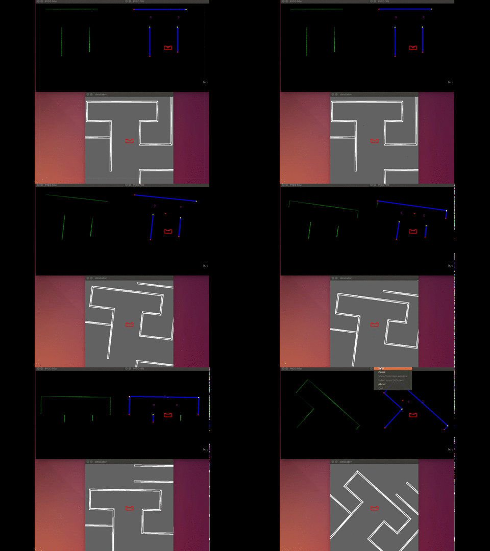
A stand-alone visualization was built to using during experiments and simulations as a debugging tool. The emc-viz tool written by Sjoerd van der Dries was used as a basis. This tool displays the robot and the LRF data points on a canvas. We decided to expand this to display the important functions and decisions of our software. The visualization eventually displayed the following things: | |||
- Hough detection lines | |||
- Detected gaps/junctions | |||
- Detected dead-ends | |||
- Setpoint used by the robot | |||
The visualization was running stand alone, which meant that while we were doing experiments the visualization ran on a computer that was subscribed the rostopics on PICO. We used the LRF data from PICO and we also created our own topic on which PICO published the setpoint he was using. This all made it possible to see what PICO ‘saw’ and ‘thought’, which made debugging very easy. | |||
The gif below shows the visualization at work. The bottom window is the simulator, the top left window is a Gaussian blurred image of the LRF data. This blur was used to apply noise reduction on the data. The top right window is the actual visualization. It shows the detected wall in blue(with endpoint in yellow and red), the used setpoint is a red dot and the dead-ends and gaps are shown in purple. | |||
[[File:viz.gif]] | |||
= Evaluating maze challenge = | |||
Sadly we weren't able to complete the maze challenge. In the first run PICO was able to take turns and did even recognize a dead end. This was, however, not a dead end with a door. After turning 180 degrees PICO was too close to the next junction. Therefore the junction could not be correctly observed and PICO thought he was driving through a corridor. When reaching the crossing PICO thought was a corridor, the mechanism for staying in the middle of the corridor kicked in and PICO drifted sideways in to the next corridor. This caused the setpoint to lie beyond the wall PICO was facing. Luckily because of the vector field PICO never bumped into the wall, but wasn’t able to drive away from it as well since we did not anticipate this problem. The second try PICO got a false setpoint when taking a turn and got stuck in the corner. This was probably due to noise on the LRF data that despite of the noise reduction and time averaging, gave a false setpoint. | |||
After the corridor challenge we noticed that the software grew rapidly with each line of code and it was decided to compartmentalized the software into different libraries in accordance with the architecture provided in Figure 1.1. Since some functions worked across different libraries and variables were redefined quite often an extra folder was created containing all the defined variables and classes to prevent double definitions and ease reusable code segments. Finally in the hope to increase the speed of the integration of different parts of the code comments were added containing the input, output and actions of the function. An example of this comment structure is shown in the snippets provided below and is used in all libraries. | |||
When looking at the performance of our software, the bottleneck was the integration of the different parts of the software even though we tried to anticipate this problem. Every piece apart; the feature detection, the drive function and taking turns, worked perfectly, but it didn’t come together. We think we began to late with the integration of all the different pieces, so that in the end we didn’t have enough time to correct the mistakes occurring during integration. We are convinced that the separate parts were working very well and that if we had some more time, we could have completed the maze challenge. Besides beginning to late with the integration, there were some design choices that impacted the result and we would have done differently next time: | |||
- '''Probabilistic Hough transform''' | |||
the probabilistic Hough transform from the openCV library seemed ideal, because instead of infinite lines it gave finite lines and their endpoints. This function later was found to be very unreliable and heavy filtering was necessary, which cost a lot of time | |||
- '''Setpoint dependence''' | |||
Driving through a maze following setpoint was very intuitive, but since the setpoints were relative to the robot we had to put a lot of effort in the simple act of taking a turn. A potential field would have been much more reliable. | |||
= Code = | |||
[https://gist.github.com/9c4249e5b5299a82914a Some function used for feature detection, explanation per function is in the comments] | |||
[https://gist.github.com/b45c4f062ac6c3dfaf9c The visualization source code] | |||
[https://gist.github.com/anonymous/3087425f709602aa8462 The driveConfigurator and setpointUpdater] | |||
== File tree == | |||
Besides the code posted above, we also wanted to point out the file structure we used throughout the project. We decided to make subdirectories in the source map for every different context. Within those context different source files were made for the different functions in that context. For example the map skill_context contained drive.cpp and hough_detect.cpp. It was agreed that it should always be clear what the input of a function was and the output of a function was. In this way everybody could work separately on the code. | |||
This method proofed very useful because of the following reasons: | |||
- It was easy to divide the code into sections on which different people could work on | |||
- The task/skill/motion framework was kept intact, so the project was always clear and organized | |||
- It was easy to change something in a certain context or function without affecting the rest of the code | |||
The file tree was arranged as follows | |||
src | |||
| | |||
| main.cpp | |||
| | |||
| | |||
+---global | |||
| classes.cpp | |||
| classes.h | |||
| CMakeLists.txt | |||
| defines.cpp | |||
| defines.h | |||
| | |||
+---interface_context | |||
| CMakeLists.txt | |||
| visualization.cpp | |||
| viz_functions.cpp | |||
| viz_functions.h | |||
| world_model.cpp | |||
| world_model.h | |||
| | |||
+---skill_context | |||
| CMakeLists.txt | |||
| detectLib.cpp | |||
| detectLib.h | |||
| drive.cpp | |||
| drive.h | |||
| hough_detect.cpp | |||
| hough_detect.h | |||
| | |||
\---task_context | |||
CMakeLists.txt | |||
task_control_fb.cpp | |||
task_control_fb.h | |||
task_control_ff.cpp | |||
task_control_ff.h | |||
task_monitor.cpp | |||
task_monitor.h | |||
Latest revision as of 13:19, 27 June 2015
Group Members
| Name: | Student id: | E-mail: |
| Ruud Lensvelt | 0653197 | g.lensvelt@student.tue.nl |
| Stijn Rutten | 0773617 | s.j.a.rutten@student.tue.nl |
| Bas van Eekelen | 0740175 | b.v.eekelen@student.tue.nl |
| Nick Hoogerwerf | 0734333 | n.c.h.hoogerwerf@student.tue.nl |
| Wouter Houtman | 0717791 | w.houtman@student.tue.nl |
| Vincent Looijen | 0770432 | v.a.looijen@student.tue.nl |
| Jorrit Smit | 0617062 | j.smit@student.tue.nl |
| René van de Molengraft | Tutor | m.j.g.v.d.molengraft@tue.nl |
Design
As a start of the course the initial design of the software is discussed. The design is divided into several parts, the general flow chart for the software design is shown in Figure 1.1. In the upcoming sections the initial design will be described.
-
Figure 1.1: Flow chart of the software design
Requirements
The goal of the maze-challenge is to solve the maze as quick as possible and without any collisions. As quick as possible is defined as solving the maze within a minimum amount of steps. The maze can be divided by discrete blocks, so every block is one step in solving the maze. The requirements to fulfill this goal are:
- The robot has to drive, which means movement in the x-, y- and theta-direction.
- The robot has to take boundaries into account to avoid a collision with walls or running into objects.
- The robot has to recognize doors to be able to found the exit of the maze.
- The robot has to be prevented from searching the same area twice, so a map of the maze will be constantly updated to be able to efficiently solve the maze.
Functions
The functions are divided into two groups: the general robot skill functions and the general robot task functions. First the three general robot skill functions are described.
- Drive functions
Realize motion of the robot by providing data to the robots actuators. Realizing the specified motion should be done using a controller to meet the requirements regarding safety.
Input: location set point. Output: motion of robot.
- Detection functions
Characterize different types of corridors based on telemetry provided by the Laser Range Finder.
Input: measured x, y and theta; Output: type of corridor.
- Mapping functions
Updates and maintains a map of the explored maze. These mapping functions can be used to check and visualize the robots actions and set new objectives.
Input: current x, y and theta of the robot; Output: new entry maze map or new robot objective.
Now the three general robot task functions are described.
- Feedback functions
Realize preventing the robot from collisions and check the position in the map to maintain safety requirements and to determine the desired new position in the maze.
Input: current x, y, theta, LFR data and objective; Output: motion of robot.
- Decision functions
Determine which direction or action the robot should take based on the map and current position.
Input: current x, y, theta and position in the map; Output: drive function initiated.
- Monitor functions
Control the exploration of the maze and prevent the robot to explore the same area more than once.
Input: current x, y and theta of the robot; Output: previous unexplored cross
The maze is viewed as a tertiary search tree in which paths represent the branches. Initial path search is done random with no particular preference for a direction and upon hitting a dead end, backtracking is initialized. Backtracking means the robot turns around at a dead end and returns to the previous decision point in the explored maze (map), meanwhile searching for a door. Upon detecting a door or reaching the point of the previous decision the robot continues its random search, or chooses the only unexplored direction at that particular point.
Components
The relevant components in the maze challenge are divided into two parts: the robot itself and the maze as the environment of the robot.
Relevant components of the robot
- Three omniwheels which make it possible to move the robot in x-, y- and theta-direction.
- Laser Range Finder to be able to detect the environment of the robot.
Relevant components of the maze
- Static walls which are the basis of the maze, those walls can form corners, crossings, T-junctions and dead ends.
- Doors which open automatically and make it possible for the robot to get access to the whole maze. Closed doors cannot be distinguished of the wall.
Specifications
Note: Almost all specifications have yet to be determined in specific numbers.
Driving speed specifications
It is unlikely that the maze can be completed with a fixed velocity. Therefore, a number of conditions need to be composed which specify the velocity and acceleration at each encountered situation. Velocity and acceleration may vary on the chosen strategy, for example to find a door (which implies a low velocity or even a drive-stop implementation) or the random walk.
- Random walk to explore an unknown part of the maze.
- Returning from a dead end to the previous decision point, meanwhile searching for a door.
- Detection of an intersection.
- Taking a particular intersection.
Changing direction
The robot can change its direction in different curvatures, at this moment the decision is made to make a full stop before the robot starts rotating. For this action the angular velocity and acceleration need to be specified.
- Determined: make a full stop before changing direction.
- Determined: change direction on a junction when the middle of the junction is reached.
- The angular velocity and acceleration during a rotation need to be specified.
Safety specifications
It is very important that the robot completes the maze without hitting the walls or running into objects. To prevent this, a safety specification should be implemented, which basically comes down to a minimal distance the robot has to maintain to its surroundings.
Laser Range Finder specifications
The Laser Range Finder has a maximal range of 30m. In order to complete the maze successfully, it is expected that this range is too large. The laser range specification to complete the maze has to be determined experimentally.
Interfaces
Regarding the interface, the obtained map from the maze should be visualized for convenient debugging of the code. Paths covered only once should be marked black. In addition, if a given branch does not lead to the exit, the robot will return to the last decision point. The path covered twice due to returning to the last decision point will be marked red.
To prevent unwanted behavior of the robot due to bugs in the software, a kill switch should be implemented in the interface such that the robot can remotely be switched off.
Initial software for corridor competition
In the initial design of the software the general framework of functions provided in Figure 1.1 is translated into a composition pattern to solve the corridor challange. The initial software consists of the skill context and task context. The skill context can be divided into two skills, the 'Drive in maze' and 'Feature detection'. The 'Drive in maze' ensures that PICO can move between the walls in the direction of a given setpoint. The 'Feature detection' detects openings in the maze, like junctions. The 'Task control' get information about the features and determines a setpoint for the 'Drive in maze' function. This software is used to complete the corridor challenge.
Drive in maze
Potential Field Method
The Potential Field Method is used to drive in a corridor. When the setpoint is determined, PICO needs to drive towards it without hitting any wall. With the Potential Field Method virtual repulsive forces are applied to PICO for every laser point. The force caused by a point depends on the distance between PICO and a laser point. The virtual force is defined as F = -1/(r^5), where F is the resulting force and r is the distance between PICO and the laser point. The force is pointing away from the obstacle. When the sum is taken over all repulsive forces, the net repulsive force is pointing away from close obstacles. The setpoint is added as attractive force, which results that PICO drives in the direction of the setpoint without hitting the wall. This Potential Field Method is also used as safety, because the repulsive forces ensure that PICO does not drive into a wall. The Potential Field Method is illustrated in Figure 2.1.
-
Figure 2.1: Potential Field Method in corridor.
Drive Function Block
Since the required action on a junction is either one of three cases, i.e. drive straight, left or right, a general drive function blocks has been implemented who’s framework can be reused for other functions. Thus though the function of a drive function block may vary depending on its goal, their overall composition is similar as the composition pattern provided in Figure 2.2. In Figure 2.2 the composition pattern is shown for a general drive function block and communication to its environment is provided through:
- Robot data provides the data the robot measures through its LRF and odometry sensors.
- Decision provides the decision from the Coordinators().
- Exception allows the drive function block to communicate to the main loop if an exceptional case occured.
Depending on the decision variable provided a drive function block either turns on or stays off. When a drive function block finishes its task it changes the parameter in Decision to the drive straight block or if it finds a condition which is outside its task description it sends an exception through the Exception variable. The general drive function block consists of four distinct parts:
- driveCoordinator() verifies whether the current situation corresponds to the required action in the decision variable, i.e. when driving straight only a straight corridor is detected, otherwise it communicates to the globalMonitor() through the exception variable. The coordinator is always vigilant on a potential command from the globalCoordinator().
- setPointUpdater() adjusts the global setpoint to compensate for the robots travelled distance the setpoint. For a detailed explanation see the next section.
- driveToSetpoint() implements the actual motion towards a setpoint using the potential field, while constantly detecting changes in the robots environment.
- driveMonitor() receives data from the setPointUpdater() and driveToSetpoint() and determines the robots current location, orientation and compares what the robot actually sees against the previously provided setpoint.
In case a turn function block is used there are extra functionalities used in the drive function block. Which are defined as
- setPathPlan() determines intermediate setpoints towards the goal setpoint to guarantee the robot turns 90 degrees into a corner. This function is only called once at the start of a turn and sets a list containing all intermediate setpoints.
- driveConfigurator() selects a setpoint from the list if has not been marked as already reached by the driveTurnCoordinator().
More information on the actual implementation can be found below.
Feature detection
Task control
In default mode the robot drives straight and while in this straight mode the hough detect returns setpoints for a corridor left, straight and right (see below). If no opening is detected from the hough detect functions the setpoint returned equals zero. The driveStraightMonitor() monitors these setpoints while in drive straight mode and has three distinct states;
- No setpoint is detected either left or right. In which case the monitor does not alter the state of the driveStraightCoordinator() by sending a message that nothing changed with respect to the default mode.
- A setpoint is detected either left or right, but it is not within range. In this case the monitor again does not alter the state of the coordinator by not sending a message.
- A setpoint is detected either left or right. In this case the monitor sends a message to the coordinator which make a decision based on all provided data from the monitor.
Drive functionality
Setpoint when Driving straight
When the robot needs to drive straight, its setpoint is initially set to the front. However, Pico will not be perfectly aligned with the walls on both sides and will not perfectly drive in the middle of those walls. To keep the right orientation and to keep the robot in the middle of the corridor throughout the challenge,the setpoint needs to be be updated. In Figure 2.3, the situation is shown when the robot is not aligned. The orientation of the robot is shown in cartesian coordinates. Under the assumption that the walls are straight, the position and orientation of these walls can be estimated with a first order polynomial approximation. This approximation is obtained using a least squares method using 20 datapoints on each side. For both sides, the distance [math]\displaystyle{ r_l }[/math] to the wall on the left side and the distance [math]\displaystyle{ r_r }[/math] to the right are determined, as well as the orientation [math]\displaystyle{ \theta }[/math]. Now, the setpoint can be updated in y-direction using these data and some basic geometric knowledge. To make the system more robust against noise, the data are averaged over the last 10 iterations. This results however in a system which reacts slower to changes in the environment. In combination with the driving function that was used, some tests showed there was too much overshoot resulting in an unstable system. Therefore, the amount of correction in [math]\displaystyle{ y }[/math]-direction was scaled with a gain with an absolute value between 0 and 1.
Setpoint when Driving a corner
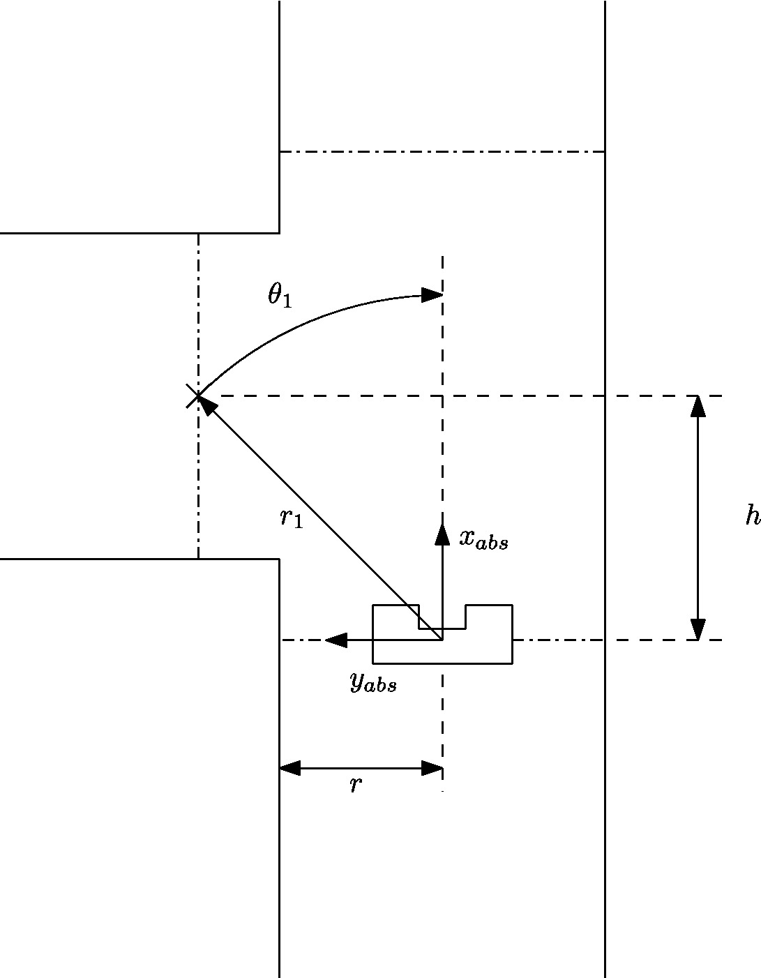
By default the robot assumes it’s in a straight corridor and upon reaching a junction the robot switches from the drive function block to a turn block. Before the turn can be made its state is logged, which act as a global marker for the starting point of the robot. The following data is logged
- Odometry data to correct the location of the setpoint with respect to the robot.
- [math]\displaystyle{ x }[/math] and [math]\displaystyle{ y }[/math] location of the middle of the selected opening.
With this data known the robot calculates intermediate setpoint along an elipsoid using a setPathPlan() function, to guarantee the robot always finishes a corner with its [math]\displaystyle{ x }[/math] axis point straight into a opening. After this initialisation the setpointConfigurator() is called in the function block to select the previously determined setpoint path sequentially. Since these setpoints are absolute with respect to the corner (they do not vary after starting a turn) the setpointUpdater() is run to update the current location of the setpoint with respect to the robot. The driveTurnMonitor() then monitors the current location based on odometry data and the currently selected setpoint from the setpointpath and returns all changed data upon reaching the setpoint to within a certain tolerance. If the setpoint is reached the driveTurnCoordinator() marks the setpoint in the list of setpoints as reached such that the setpointConfigurator() knows to select the next setpoint from the list. The code for the turn then corresponds to
- turnInitialize()
- setPathPlan()
- setpointConfigurator()
- setpointUpdater()
- driveTurnMonitor()
- driveTurnCoordinator()
The fashion in which the setpoint is updated with respect to the robot in the setpointUpdater() is described next. The initial starting point of a turn, i.e. in which data is logged, is shown in Figure 2.4.
Since the robot’s coordinate frame is relative, the previously determined global marker is used to determine the travelled distance and the robot’s orientation. With this data the global setpoint is translated to the robot’s relative frame according to
[math]\displaystyle{ r_2=r_1-dr, }[/math]
[math]\displaystyle{ \theta_2=\theta_1-d\theta. }[/math]
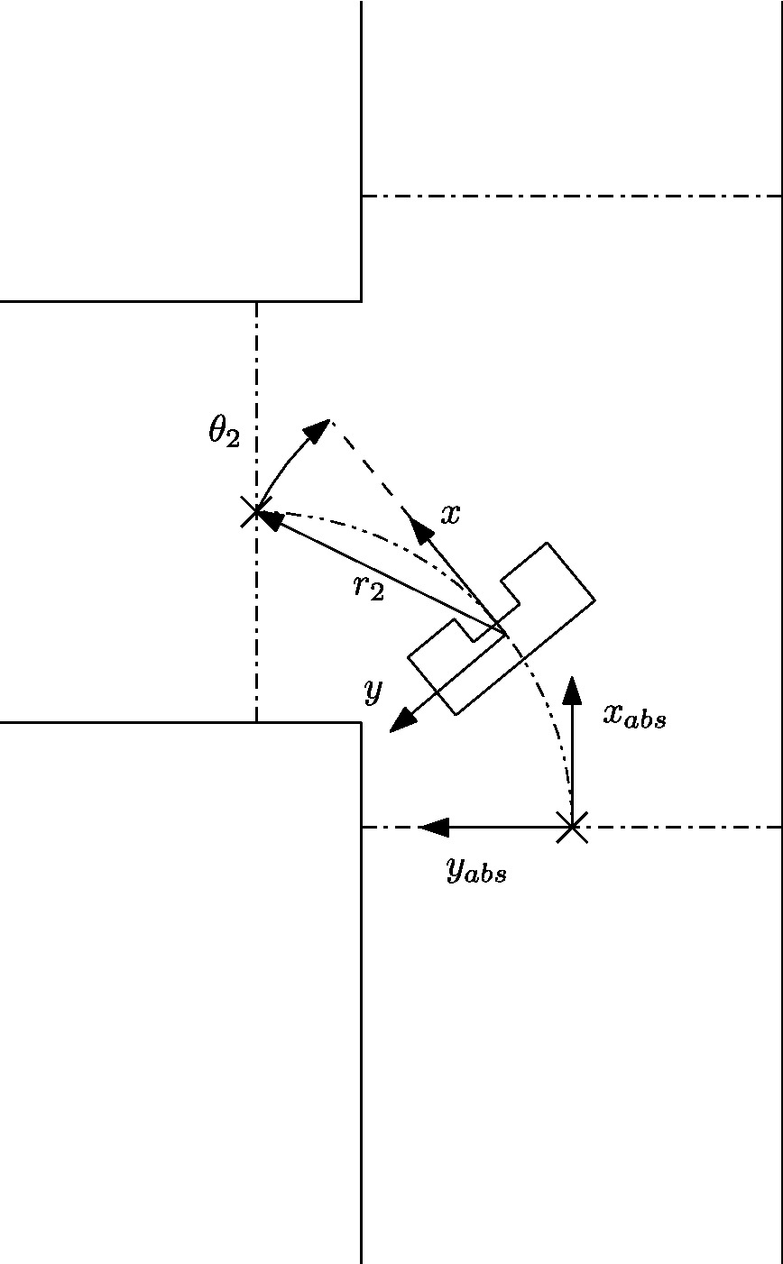
The effect of this update is that the setpoint varies in position when observing it from the robot while it stays at the same location with respect to the absolute marker. An intermediate step in driving through a corner can be seen in Figure 2.4.
Since the robot needs to end up in a corridor with its [math]\displaystyle{ x }[/math]-axis aligned with the corridor it is entering both [math]\displaystyle{ x }[/math] and [math]\displaystyle{ y }[/math] coordinates are required to be met to within a certain tolerance [math]\displaystyle{ tol }[/math], i.e.
[math]\displaystyle{ y-\Delta S_y\lt tol. }[/math]
[math]\displaystyle{ x-\Delta S_x\lt tol. }[/math]
Upon completion of a turn the robot jumps back to driving in its default mode and using the above it is guaranteed that the robot crosses the line in Figure 2.5 upon exiting the turn. Since the odometry data is marked global the axis to determine this [math]\displaystyle{ \Delta S }[/math] changes as the robot takes multiple turns to the left or right. In order to take this into account a counter for the amount of left and right turns is set every time a corner is successfully finished and the difference between which determines which axis of the odemetry data is either [math]\displaystyle{ x }[/math] or [math]\displaystyle{ y }[/math].
Evaluating corridor challenge
PICO managed to finish the corridor challenge. With a time of 21 seconds, we finished at the fourth place. The potential field ensures that PICO did not bump into walls, the corner of the exit was detected and PICO take this corner. However, PICO did not take the corner in a smooth way, because the setpoint in the exit was not at a fixed place. This error is solved after the competition.
Further improvements:
- The function setPointUpdater needs to be updated with LRF data. In the old version the odometry data was used.
- During the corridor competition a fixed gain was used to increase the length of the resulting force of the potential field. This gains needs to be replaced by a function that is dependent on the width of the corridor.
Software for maze challenge
Feature detection
To safely navigate through the maze, the robot must be aware of its surroundings. While during the corridor challenge we only used the rough laser data to determine distances en detect openings, we started to develop a new technique for the maze challenge. This technique makes use of the Hough transform, available in the OpenCV-libary. The Hough transform is a technique to determine lines through noisy data, which is generated by our sensors. With this technique, the robot is able to determine all the walls as lines instead in points. This makes it a lot easier and robuster to determine openings in corridors, junctions and turns.
To achieve the best result in real time the LRF data was filtered with a gaussian blur, to apply noise reduction. After that duplicate lines were filtered. This gave a robust way of determining the walls around the robot.
To determine openings in a robust way, the lines are represented by a polar coordinate system, depicted in figure 2.6. In this figure, r is the shortest distance from the origin (which is at the robot) to that line, and [math]\displaystyle{ \theta }[/math] the angle that line makes with the robot. If the lines are represented in this way, it become easy to compare different lines with each other and independent of the orientation of the robot.
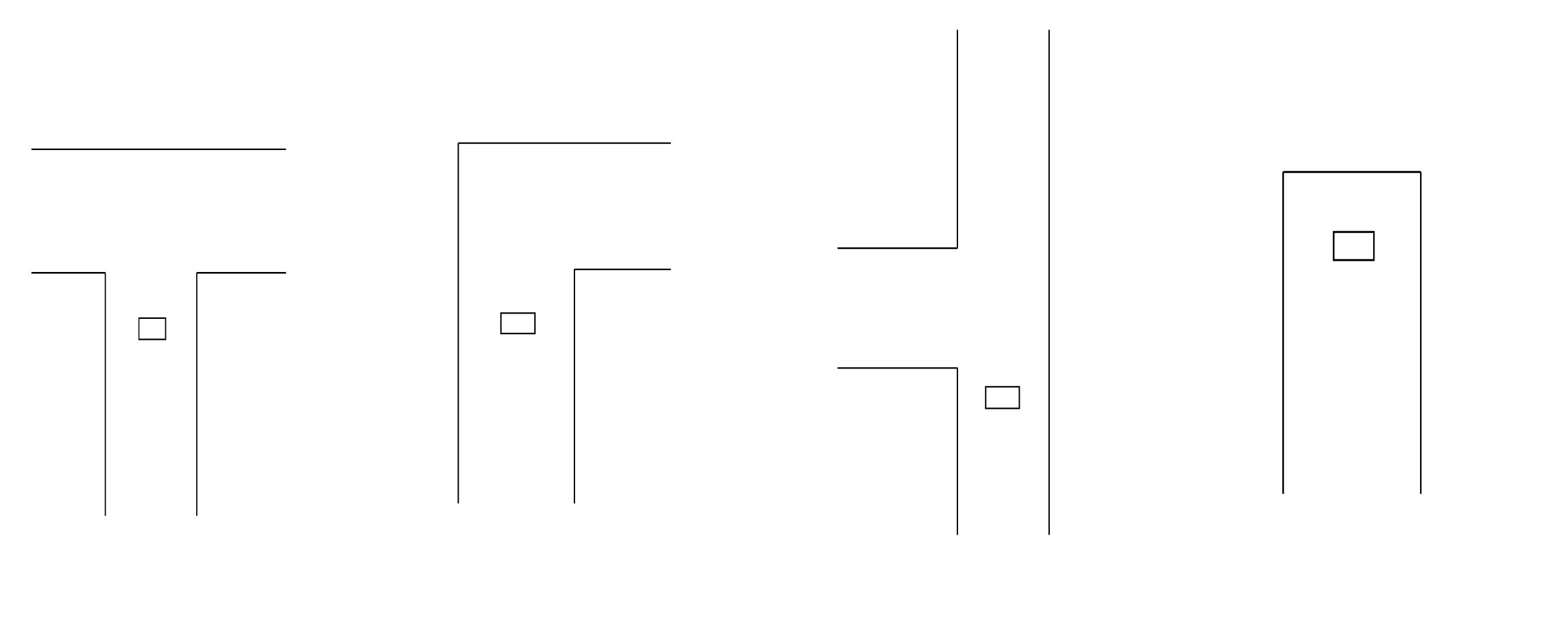
When simply driving in a corridor the robot detects two parralel lines, one to the right and one to the left. If for instance a T-junction is considered like the one below, the robot sees two parallel lines and one line perpendicular to those two that is not directly connected to the two parallel lines. If this situation arises, the robot immediately knows what kind of crossing it has to deal with. The same holds for the other possible junctions. The turn detection relies on the fact that the one of the parralel lines that the robot sees is suddenly connected with a line perpendicular to it. This means that the opening is at the other side. The image below also depicts a corridor with an opening. If the robot has detect two parallel lines but one has an interruption, it knows it has to deal with an opening. The same holds for a complete crossing with four roads, it just has to detect an extra interruption to the right. At last The dead-end detection is very similar to the first T-junction detection. The robot sees two parallel lines and one perpendicular to it. The only difference is that all lines must be connected for it to be an dead-end.
Door handling/detection
In feature detection dead ends will be detected, each dead end could be a possible door. The dead end detection places a setpoint just before the possible door, the robot drives to this setpoint. This setpoint is located such that the robot will be in the door area. When the setpoint is reached all velocities are set to zero and the door request is executed. Five seconds after this request feature detection is used to check if a possible door has opened. If this is the case the robot will drive straight through the corridor. If no door has opened, the robot will turn 180 degrees, the history will be updated and the Tremaux algorithm decides what the next action will be.
Maze mapping/strategy
Determine orientation of the robot
Since the maze is constructed out of corners of 90 degrees, an integer multiple of this value is used to determine the orientation of the robot. The initial orientation is zero degrees, hence the decision at every subsequent junction is added to the initial orientation value. A counter clockwise structure has been applied, resulting in +90 degrees for a left turn, +180 degrees for going back the same path as the driving direction, +270 degrees of a right turn and +0 degrees for straight ahead driving over the junction. When the orientation value is larger or equal to 360 degrees, 360 degrees is subtracted. By keeping track of the orientation at every corner and junction, the orientation relative to the initial orientation is known at all times.
Determine orientation number
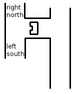
By driving through the maze, changes are detected based on measured data by the developed detection software. The detection software also communicates what type of situation is detected, for example a T-junction. However, the situation is communicated relative to the current driving direction, so for example if the detection software outputs a T-junction with left en right possibilities, it is possible that it actually is a T-junction in north and south direction. This situation is depicted in Figure 2.5. To obtain usable data for the maze history, the information from the detection software is corrected with a correction number, which basically shifts the information a given amount of places. The number of shifts is determined by the current orientation: 1 for a current orientation of +90 degrees, 2 for a current orientation of +180 degrees, 3 for a current orientation of +270 degrees and 0 for a current orientation of 0 (or 360) degrees. Now all the junctions can be mapped in global wind direction names: North, East, South and West.
Maze history
The maze history is a vector of classes. Each entry of the vector belongs to a node ID number. Because of the work done in the orientation determination functions above, the maze history function is a matter of bookkeeping and initialization. When the program is started, the straight ahead direction is set to North which is now the global North for the entire maze. Mapping the maze all starts with a detected change in the maze from detection software, which triggers the following actions:
- Only when the [math]\displaystyle{ 1^{st} }[/math] node is detected: Initialize first node by setting the south exploration value of the [math]\displaystyle{ 1^{st} }[/math] junction to explored. This implies that the initial driving direction is from south to north, regardless of the ´real´ direction.
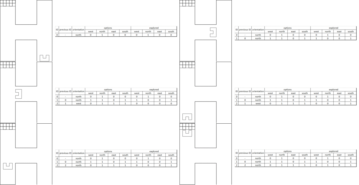
- A node is added to the history vector by the push_back functionality for each detected change in the maze. This results in an expanding history vector. In each entry the global coordinates of the node are saved together with information regarding the available possibilities, e.g. West, North, East and/or South opening. Next, for a new node, the exploration options are initialized. Now the current options for the junction at hand is returned to the Tremaux algorithm, e.g. the unexplored possibilities are returned.
- When a next node is created because of a change in the maze is detected, the explored options from the previous node based on the decision made by the Tremaux algorithm are updated. This way the maze history stays up to date.
- If there is a loop in the maze, a node could be visited multiple times. To prevent taking the same decision, the global position of a detected junction is compared with the already detected junctions in the history. If it appears to be a new junction, a new node is created. However, if it turns out that the junction has been visited before the concerning node information is used from the history. Using the Tremaux algorithm, the same (incorrect) decision can not be made twice.
A graphical presentation of the maze history in action is depicted in Figure 2.6.
Visualization
A stand-alone visualization was built to using during experiments and simulations as a debugging tool. The emc-viz tool written by Sjoerd van der Dries was used as a basis. This tool displays the robot and the LRF data points on a canvas. We decided to expand this to display the important functions and decisions of our software. The visualization eventually displayed the following things:
- Hough detection lines
- Detected gaps/junctions
- Detected dead-ends
- Setpoint used by the robot
The visualization was running stand alone, which meant that while we were doing experiments the visualization ran on a computer that was subscribed the rostopics on PICO. We used the LRF data from PICO and we also created our own topic on which PICO published the setpoint he was using. This all made it possible to see what PICO ‘saw’ and ‘thought’, which made debugging very easy.
The gif below shows the visualization at work. The bottom window is the simulator, the top left window is a Gaussian blurred image of the LRF data. This blur was used to apply noise reduction on the data. The top right window is the actual visualization. It shows the detected wall in blue(with endpoint in yellow and red), the used setpoint is a red dot and the dead-ends and gaps are shown in purple.
Evaluating maze challenge
Sadly we weren't able to complete the maze challenge. In the first run PICO was able to take turns and did even recognize a dead end. This was, however, not a dead end with a door. After turning 180 degrees PICO was too close to the next junction. Therefore the junction could not be correctly observed and PICO thought he was driving through a corridor. When reaching the crossing PICO thought was a corridor, the mechanism for staying in the middle of the corridor kicked in and PICO drifted sideways in to the next corridor. This caused the setpoint to lie beyond the wall PICO was facing. Luckily because of the vector field PICO never bumped into the wall, but wasn’t able to drive away from it as well since we did not anticipate this problem. The second try PICO got a false setpoint when taking a turn and got stuck in the corner. This was probably due to noise on the LRF data that despite of the noise reduction and time averaging, gave a false setpoint.
After the corridor challenge we noticed that the software grew rapidly with each line of code and it was decided to compartmentalized the software into different libraries in accordance with the architecture provided in Figure 1.1. Since some functions worked across different libraries and variables were redefined quite often an extra folder was created containing all the defined variables and classes to prevent double definitions and ease reusable code segments. Finally in the hope to increase the speed of the integration of different parts of the code comments were added containing the input, output and actions of the function. An example of this comment structure is shown in the snippets provided below and is used in all libraries.
When looking at the performance of our software, the bottleneck was the integration of the different parts of the software even though we tried to anticipate this problem. Every piece apart; the feature detection, the drive function and taking turns, worked perfectly, but it didn’t come together. We think we began to late with the integration of all the different pieces, so that in the end we didn’t have enough time to correct the mistakes occurring during integration. We are convinced that the separate parts were working very well and that if we had some more time, we could have completed the maze challenge. Besides beginning to late with the integration, there were some design choices that impacted the result and we would have done differently next time:
- Probabilistic Hough transform
the probabilistic Hough transform from the openCV library seemed ideal, because instead of infinite lines it gave finite lines and their endpoints. This function later was found to be very unreliable and heavy filtering was necessary, which cost a lot of time
- Setpoint dependence
Driving through a maze following setpoint was very intuitive, but since the setpoints were relative to the robot we had to put a lot of effort in the simple act of taking a turn. A potential field would have been much more reliable.
Code
Some function used for feature detection, explanation per function is in the comments
The driveConfigurator and setpointUpdater
File tree
Besides the code posted above, we also wanted to point out the file structure we used throughout the project. We decided to make subdirectories in the source map for every different context. Within those context different source files were made for the different functions in that context. For example the map skill_context contained drive.cpp and hough_detect.cpp. It was agreed that it should always be clear what the input of a function was and the output of a function was. In this way everybody could work separately on the code.
This method proofed very useful because of the following reasons:
- It was easy to divide the code into sections on which different people could work on
- The task/skill/motion framework was kept intact, so the project was always clear and organized
- It was easy to change something in a certain context or function without affecting the rest of the code
The file tree was arranged as follows
src
|
|   main.cpp
|
|
+---global
|       classes.cpp
|       classes.h
|       CMakeLists.txt
|       defines.cpp
|       defines.h
|
+---interface_context
|       CMakeLists.txt
|       visualization.cpp
|       viz_functions.cpp
|       viz_functions.h
|       world_model.cpp
|       world_model.h
|
+---skill_context
|       CMakeLists.txt
|       detectLib.cpp
|       detectLib.h
|       drive.cpp
|       drive.h
|       hough_detect.cpp
|       hough_detect.h
|
\---task_context
       CMakeLists.txt
       task_control_fb.cpp
       task_control_fb.h
       task_control_ff.cpp
       task_control_ff.h
       task_monitor.cpp
       task_monitor.h
