Viotar/Quantifying the signal: Difference between revisions

From Control Systems Technology Group
Jump to navigation Jump to search
No edit summary
No edit summary
 
(76 intermediate revisions by 4 users not shown)
Line 1: Line 1:
The signal that we want from the string, somehow will have to be read out by the instrument. No matter how this is done, some sensor will provide a signal, in which the vibration we want from the string should be recognised. This recognising has to be done on a reliable, quantitative basis. More specifically, there has to be some kind of scalar quantity that gives us how far we really are from the ideal trajectory in the bow speed-force space, so a feedback loop can be made to let the system find this trajectory for itself. For this, an experiment will be done, and it's results will be analysed thoroughly.
{|cellpadding="10"
|-valign="top"
|width="100%" style="border:1px solid #fabd23; background-color:#FEF5DE;text-align: justify;"|
{| padding="0" cellspacing="0" style="margin-top:.2em; width:100%; background:none"
| rowspan="32" width="5px" |
| rowspan="2" class="BGorange1" valign="middle" style="text-align:center; padding:.6em 10px .6em 10px; background-color:#A9D0F5; border-top:2px solid #2E9AFE; border-bottom:2px solid #2E9AFE" |
<h1 style="font-size:180%; border:none; margin:0; padding:0">
'''Software design - Quantifying the signal
'''
</h1>
<div style="position:relative; top:.25em; font-size:100%">'''<br/>William Schattevoet<br/>David Duwaer<br/>Eric Backx<br/> Arjan de Visser'''</div>
| rowspan="32" width="10px" |
| rowspan="32" width="5px" |
|-
|
|-
| valign="top" rowspan="30" style="padding:1em 10px 0 10px" |
|}
<br/>
{| cellpadding="10"
|-valign="top"
|width="49%" style="border:2px solid #d73430; background-color:#FBEAEA"|
<h1 style="font-size:180%; border:none; margin:0; padding:0">
'''Subpages:'''
</h1><br/>
{{:Viotar_Menu}}


==Experiment plan==
- Is the computer model of the bowed string accurate?


- Where does the "pleasant" sound come from that you hear when you stand next to the instrument when it's bowed? Is it mainly the vibration of the body that you hear? In that case it would origin mainly from the pressure variances of the string on the bridge, which translate into the body. On the other hand, it could be mainly the vibration of the string that you hear. In that case, the transversal wave as described by the computer model and measured by a laser sensor is dominant. The outcome of this will be important in the choice of what the capture and amplify exactly, when the instrument is done.  
|width="2%" style="background-color:#FEF5DE;"|
|width="49%" style="border:2px solid #fabd23;text-align: justify;"|
<h1 style="font-size:180%; border:none; margin:0; padding:0">
'''Overview:'''
</h1><br/>
The signal that we want from the string, somehow will have to be read out by the instrument. No matter how this is done, some sensor will provide a signal, in which the vibration we want from the string should be recognised. This recognising has to be done on a reliable, quantitative basis. More specifically, there has to be some kind of scalar quantity (which we'll define as the tonal quality Q) that gives us how far we really are from the ideal trajectory in the bow speed-force space, so a feedback loop can be made to let the system find this trajectory for itself. For this, an experiment will be done, and it's results will be analysed thoroughly.


- What does the vibration we want (Helmholtz) look like in the transversal wave of one point of the string?


- What does the vibration we want (Helmholtz) look like in the pressure variances of the string on the piëzo element?
|}<br/>
{| cellpadding="10"
|-valign="top"
| style="border:2px solid #00FF33; background-color:#CCFF99"|
==Software Design (Quantifying the signal we want to see)==
With software design, we mean the way the controller is structured. There are many possibilities, but it is important to design the controller in such a way that it matches the requirements that are stated. The controller will be tested on a fixed point model of the string, so it is also important to verify that the model is accurate enough to represent the real string. Besides that, also the following questions need to be answered to come to a good software design:


* Where does the "pleasant" sound come from that you hear when you stand next to the instrument when it's bowed? Is it mainly the vibration of the body that you hear? In that case it would origin mainly from the pressure variances of the string on the bridge, which translate into the body. On the other hand, it could be mainly the vibration of the string that you hear. In that case, the transversal wave as described by the computer model and measured by a laser sensor is dominant. The outcome of this will be important in the choice of what the capture and amplify exactly, when the instrument is done.


A measurement will be done for the low E-string and the high e-string, on the open string and the 1st, 12th and 13th fret. The open string and 1st fret measurements are needed to "shift" the signal in the frequency domain. Everything that shifts up according to the fret change is part of the vibration we want to measure, the rest is noise. With this principle we are hoping to be able to cancel the noise from the measurements. The 12th and 13th fret are done so that the same can be done for a much higher position (one octave up), because the waveform may have a different character there.
* What do the following vibrations look like for different types of measuring instruments?
** The "pleasant" vibration we want (Helmholtz)
** Raucous noise (bow pressed too hard against the string)
** Surface sound (bow pressed too softly against the string)


==Goal of the measurement==
* How can we recognize a pleasant (Helmholtz) vibration in time and/or frequency domain?
In order to find out what a Helmholtz vibration and a noisy (in this case raucous) sound look like in the frequency domain, we did some experiments. We measure the vibration of the string in three ways. Firstly, we measure the transversal motion of the string, using a laser. This will be done because we need to know the vibration of the string at one single point, since the model also describes one point. Also the vibration at the bridge will be measured, using the existing piëzo’s. This is done because we want to know the difference between the vibration of the end of the string and the vibration at a single point somewhere in the middle of it. At last, we also measure the sound that you hear when the instrument is bowed, using a microphone. The main goal of these measurements is that we want to know how we can recognize a clear Helmholtz vibration in the frequency domain.


==Measurement setup==
* What kind of controller do we need to meet all of our requirements?
The measurement with the laser will be done using a Lab Interface. For the measurements with the piëzo’s and the microphone, we will use a SigLab. The experiments will be done for two different strings, the A and B string. The string will be bowed at 4 different fret positions, being the open string, the 1st, 12th and 13th fret. All the measurements will be done twice to reduce errors.


==Results==
In order to answer these questions, some experiments have been done. These experiments give information about what a bowed string looks like in both time and frequency domain. When we are able to find out how to recognize a pleasant (Helmholtz) sound from time and/or frequency information, this is a first step in designing an appropriate controller.
In figure 1 both the time and frequency domain results are given for what we call a raucous sound, which means that the string is sticking to much. This measurement is done using a piëzo. As can be seen from the power spectrum, there are no harmonic vibrations in this sound. It is all very chaotic and there is only noise.
[[File:Krassen.png|frame|Border|left|Figure 1: The measurement results for a raucous sound]]


===Experiment===
To measure Helmholtz motion, a measurement will be done for the A-string and the B-string, on the open string and the 1st, 12th and 13th fret. The open string and 1st fret measurements are needed to "shift" the signal in the frequency domain, when necessary. Everything that shifts up according to the fret change is part of the vibration we want to measure, the rest is noise. With this principle we are hoping to be able to cancel the noise from the measurements. The 12th and 13th fret are done so that the same can be done for a much higher position (one octave up), because the waveform may have a different character there.


To measure raucous noise and surface sound, only the open A- and B-string will be measured. That is, beacause we only want to know what these signals look like and we do not actually use them.


====Experiment goal====
The goal of this experiment is to find out what a Helmholtz vibration and a noisy (surface or raucous) sound look like in frequency and time domain. We measure the vibration of the string in three ways. Firstly, we measure the transversal motion of the string, using a laser. This will be done because we need to know the vibration of the string at one single point, since the model also describes one point. Also the sound that you hear when the instrument is bowed is measured using a microphone. At last, the vibration at the bridge will be measured, using the existing piëzo’s. This is done because of two reasons. Firstly, we want to know the difference between the vibration of the end of the string and the vibration at a single point somewhere in the middle of it. The second reason is that the piëzo’s seem to be the best way to pick up the signal for the controller because these piëzo’s are also used as pick up element in normal electric guitars. The main goal of these measurements is that we want to know how to recognize a clear Helmholtz vibration in the frequency domain. Also the time domain information will be important, but the results for a clear Helmholtz vibration are pretty obvious here.


==Analysing the results==
====Experiment setup====
The measurement with the laser will be done using a Laboratory Interface. For the measurements with the piëzo’s and the microphone, we will use a SigLab. The experiments will be done for two different strings, the A and B string. The string will be bowed at 4 different fret positions, being the open string, the 1st, 12th and 13th fret. All the measurements will be done twice to reduce errors.


The first goal was to cancel the noise from the measurements using the method explained in the previous paragraph. This proved to be impossible. The power spectrum of a measurement may be split up in two components: the 'noise' component, which stays the same when a higher note is played, and the 'harmonic' component, which shifts up when a higher note is played.
====Results====
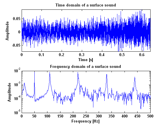
In figure 1 both the time and frequency domain results are given for what is called a raucous sound, which means that the string is sticking to much. This measurement is done using a piëzo guitar pickup. As can be seen from the power spectrum, there are no harmonic vibrations in this sound. It is all very chaotic and there is only noise. In figure 2 the results are given for what is called a surface sound, which means that the bow force is to low and the bow scratches along the string.  In this figure there are some peaks that are clearly higher than others. These are the hormonic frequencies for a Helmholtz vibration as we will see later. Beside those peaks however, there is also a lot of noise in between them. This noise could be a thing that makes a surface sound recognisable later on.


Probaby, Helmholtz is the only harmonic vibration that you can get from a string when you bow it. With a bow you can never get a normal standing wave as when you would pluck the string. Because of this, it is not necessary to quantify "how much" the measured vibration is the specific Helmholtz waveform. It may suffit to merely quantify how harmonic the measured vibration is. This can be done by detecting the fundamental frequency in the fft of the signal, and looking looking how many multiplications of this frequency are still in the signal. The more overtones, the sharper the Helmholtz, and therefore the better the tone.
[[File:Raucous.png|left|frame|Border|Figure 1: The measurement results for a raucous sound]]
 
[[File:Surface.png|center|frame|Border|Figure 2: The measurement results for a surface sound]]
 
 
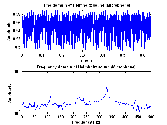
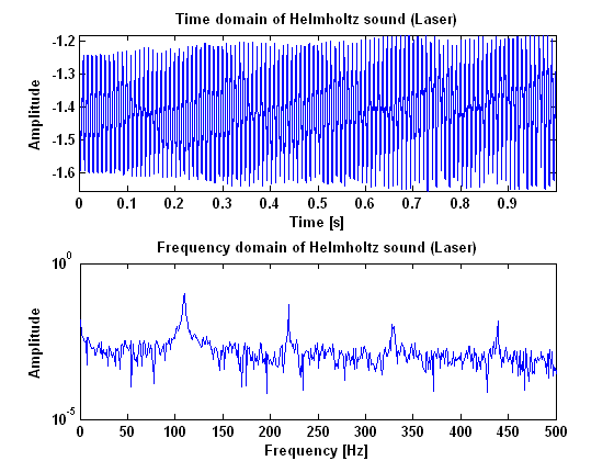
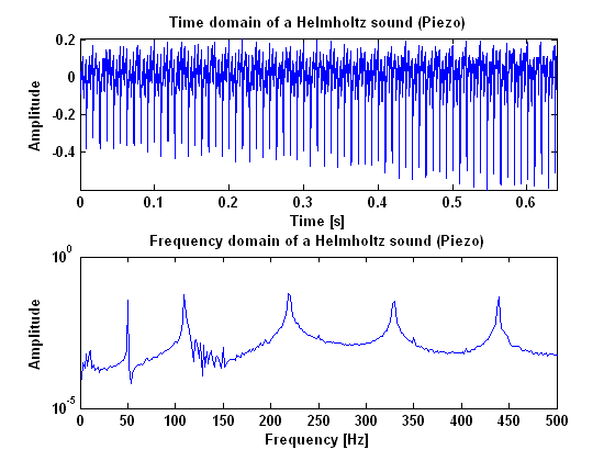
In figures 3, 4 and 5, the results are given for helmholtz vibration, measured with the microphone, the laser and the piëzo. As can be seen in these figures, a Helmholtz vibration gives clear harmonic peaks in the power spectrum. Especially the measurements done with the piëzo and the laser give a good result. Important to notice when the vibration is measured with the piëzo, is the peak at 50 Hz which is caused by the power supply. Beside that peak however, all the peaks appear in harmonic frequencies. When the result is compared to the result of the surface sound, it is clear to see that there is a lot less noise in a Helmholtz vibration. This may be very important in recognizing the type of the vibration and, more imporatant, make the difference between a surface sound and a helmholtz sound visible.
 
[[File:Helmholtz_microfoon.png|frame|Border|left|Figure 3: The measurement results for a Helmnholtz sound measured with a microphone]]
 
[[File:Helmholtz_laser.png|frame|Border|center|Figure 4: The measurement results for a Helmnholtz sound measured with a laser]]
 
[[File:Helmholtz_piezo.png|frame|Border|center|Figure 5: The measurement results for a Helmnholtz sound measured with a piëzo]]
 
====Noise cancellation====
The first goal was to cancel the noise from the measurements using the pitch shifting method explained in the experiment plan. This has proved to be not as simple as we have thought. The power spectrum of a measurement may be split up in two components: the 'noise' component, which stays the same when a higher note is played, and the 'harmonic' component, which shifts up when a higher note is played. They may be written as <math>p_n</math> and <math>p_h</math>, respectively, so that <math>p=p_h+p_n</math>. The two measurements are called '1' and '2', of which '1' will be pitch-shifted towards the pitch of '2'. The shifted measurement is called 's'. will yield these equations:
 
*<math>p_1=p_{h,1}+p_{n,1}</math>
 
*<math>p_2=p_{h,2}+p_{n,2}</math>
 
*<math>p_s=p_{h,s}+p_{n,s}</math>
 
*<math>p_{h,s}=p_{h,2}</math>
 
These are 4 equations with 6 unknowns, so the system can't be solved. Therefore, the measurements of the 1st and 13th frets are dropped, because they are now only excess measurements.
 
===Controller Design===
====Possible controller architectures====
 
Before we can decide what type of controller would be best for our system, let's take a look at the possible controller architecture. The first type of controller is open loop (feed forward). This means that the controller only sends a signal to actuators without checking whether the desired requirements are achieved or not. The second architecture is a closed loop (feedback) controller. This controller compares a measured value with a pre-defined value and adapts the system, untill the measured value equals the pre-defined value. At last, there is a combination of both. In this controller, all the known information is used to send a feed forward signal to bring the system as close as possible to the desired state. The small changes are made using the feedback signal. This controller is generally preferred above the feedback only controller because controlling on the feedback signal is mostly rather slow.
 
Reflected on our viotar, this gives the following concepts:
 
* Feed forward:
All the values for bow speed and force are pre-defined in a look-up table for every fret. From the obtained signal, the fundamental frequency of the vibration can be determined, which is directly related to the played fret. After that, the controller looks up the right values for bow speed and force and uses it as controlvalues.
 
* Feedback:
The obtained signal is compared with an ideal Helmholtz signal, and a “tone quality” is assigned. Using this rating as a feedback quantity, a closed loop is created with the goal to get an ideal Helmholtz signal from the string.
 
* Feed forward and feedback:
First, the right bow force and speed are determined using the lookup table, and actuated. Then, the comparison with the ideal Helmholtz signal starts, creating a feedback loop using this “tone quality”. This feedback signal is only used for fine-tuning the bow force and speed.
 
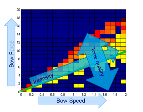
A combination of feed forward and feedback theoretically leads to the best result. That's why we choose to work this concept out first. In theory this means that tone intensity and quality will be controlled in the way shown in figure 6. In order to do that, we need to be able to recognize Helmholtz and quantify the signal. This can be done in both time and frequency domain as we will see later.
 
[[File:controller_int_quant.PNG|frame|Border|center|Figure 6: Quality and intensity paths]]
 
====Recognising Helmholtz and quantifying the signal====
Probably, Helmholtz is the only harmonic vibration that you can get from a string when you bow it. With a bow you can never get a normal standing wave as when you would pluck the string. Because of this, it is not necessary to quantify "how much" the measured vibration is the specific Helmholtz waveform. It may suffit to merely quantify how harmonic the measured vibration is. This can be done by detecting the fundamental frequency in the Fourier transformation of the signal, and looking how many multiplications of this frequency are still in the signal. The more overtones, the sharper the Helmholtz, and therefore the better the tone.
 
In order to do this we made amplitude plots in the frequency domain. This gives information about the frequencies at which high peaks appear and what their amplitudes are. We did this for the model as well as for our measurements. When we first analyzed the model, we seemed to be right in the fact that as the tone gets better, more peaks appear in the power spectrum. These peaks are not randomly spread out, but appear at harmonic frequencies. That is, at n-times the fundamental frequency with n being the number of the peak. This is also made visible in the figures below. These figures show the difference between the frequency that you would expect following this rule and the actual frequency that comes out of the model. For an unidentifiable tone, there are no harmonic tones on the expected frequencies, as the graph runs out of the figure. For a clear Helmholtz vibration however, the rule is satisfied for nine peaks. A second thing that becomes clear by analyzing the results from the model, is that the amplitude of every next peak decreases exponentially.
 
[[File:Model_unidentifiable.PNG|frame|Border|left|Figure 7: Amplitude ratio and frequency errors for an unidentifiable sound]] [[File:Model_helmholtz.PNG|frame|Border|center|Figure 8: Amplitude ratio and frequency errors for a Helmholtz vibration]]
 
 
When we take a look at the measurements results, it becomes clear that these measurements are not as “clean” as the model. The same figures as for the model are also made for the measurements, as you can see below. The amplitude of the peaks does indeed decrease more or less exponentially as we would expect from the model. The number of peaks that appear at the expected frequency however, is only three for a vibration that sounded like a clear Helmholtz vibration to us. This can be explained by the fact that these measurements are done using a piezo element and the string vibrates along this element instead of perpendicular to it, which gives another signal. This problem is going to be solved however, because in the meantime experiments have proofed that the signal gets better when the string vibrates perpendicular, like it will on our prototype.
 
[[File:Metingen_helmholtz.PNG|frame|Border|center|Figure 9: Amplitude ratio and frequency errors for measured Helmholtz sound]]
 
So, we seemed to be right in the fact that a vibration being Helmholtz has something to do with the frequencies at which harmonic peaks appear and the amplitude of that peaks compared to that of the fundamental frequency. There is only one important thing that makes this method of quantifying the signal irrelevant for our prototype control system. The point is that for this method a Fourier transformation needs to be done in the control unit in order to detect what the quality of the signal is. The problem is, that a Fourier transformation cannot be done instantaneously but only when enough information about the vibration is gathered. A simple rule tells that the resolution of the transformation equals 1/(sample time). In our case, where quality of the sound depends strongly on the exact frequencies where peaks appear, we should have a resolution in the frequency domain of at least 1 Hz. This means that the sample time for every transformation needs to be about a second, while the vibration needs to be adapted in several milliseconds up to several hundreds of seconds at most. So, this method is simply never going to satisfy our requirements.
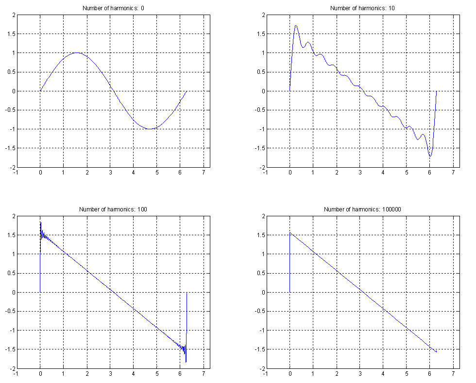
However, there is another way to perform this method, being in the time domain. When we take a look at the sawtooth like waveform of a Helmholtz vibration, we can already in the time domain draw some conclusions regarding to the quality of the vibration. The reason for this is that the harmonic peaks in the time domain, with their decreasing amplitudes, and the saw-toothed waveform in the time domain are strongly related to each other. A saw-toothed waveform essentially is a set of harmonic sinuses with decreasing amplitudes, being sharper when more harmonic sinuses are present. Putting this in an equation leads to the following expression for the signal, consisting of n harmonics:
 
<math>f=\sum_{i=1}^{n}(1/n)  sin(nt)</math>
 
So the fact that more harmonic peaks appear in the frequency domain, finds is origin in the fact that more harmonic sinuses occur in the time domain. Moreover, when we want to quantify the signal in the time domain on the same properties as we did in the frequency domain, we only have to assess the signal on its sharpness. To proof this theory, figure 10 shows how the shape of the signal changes as the number of harmonic sinuses is increased. This leads to a perfectly sharp saw tooth, when the number of harmonic sinuses goes to infinity.
 
[[File: Sawtooth_x4.PNG|frame|Border|center|Figure 10: Sawtooth signals for an increasing number of harmonics]]
 
 
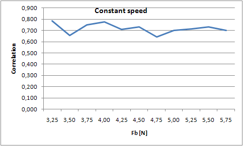
So, the idea is that we quantify the signal on the sharpness of the sawtooth. In order to do this we adapted our model and added a possibility to generate a sawtooth that serves as a reference. The correlation between the signal and our auto-generated reference sawtooth will be used as the quantification. This method will reduce the sample time to the longest period in the signal, which is 1 devided by the lowest frequency present in the signal. In this case the lowest frequency is about 100 Hz, so the sample time is about 10 milliseconds. To find out whether the signal indeed can be quantified on its sharpness (and thuss number of harmonics), we did some experiments. In the Helmholtz region, we varied the bowing speed at a constant bowing force and varied the bowing force at a constant speed. For all these simulations the correlation is calculated and plotted in the figures below (figures 11 and 12). From these figures, it can easily be concluded that there is not an ideal combination of bowing speed and force. That is, there is not an optimum which gives the best Helmholtz vibration. This means that when the vibration is a so called Helmholtz vibration, the system cannot be controlled to a point at which the correlation is highest. That is why we choose to make a lookup table with combinations of bowing speeds and forces that are in the Helmholtz region. The control unit then only needs to identify the fundamental frequency and lookup the right settings for the bowing speed and force. This gives great advantages regarding to adaptation time, because the controlling time now reduces to one sample time.
 
[[File:Constant_force.PNG|frame|Border|left|Figure 11: Correlation for varying bowing speeds]] [[File:Constant_speed.PNG|frame|Border|center|Figure 12: Correlation for varying bowing forces]]
 
====Controller concept====
The process described above, brought us to a controller design for the prototype. This controller makes use of a look-up table. This look-up table contains all the pre-defined values for bowing speed and force. By determining the fundamental frequency of the signal, the controller "knows" which fret is played and therefor what values for bowing speed and force are required. To make sure that the bowing speed indeed equals the value from the look-up table (also under varying bowing force) the engine speed is measured using an encoder and looped back to the controller. For the bowing force this does not seem to be neccesary, since the bowing force does not depend on the bowing speed.

Latest revision as of 14:58, 23 March 2011

Software design - Quantifying the signal


William Schattevoet
David Duwaer
Eric Backx
Arjan de Visser


Subpages:


Main page

Working principle of the violin and predicting it’s behavior

Ways to exite the string

Hardware Design

Software Design (Quantifying the signal we want to see)

Realisation and Proof of concept

Patent Research

Background information: Interview with Hendrick Zick

Recommendations


Overview:


The signal that we want from the string, somehow will have to be read out by the instrument. No matter how this is done, some sensor will provide a signal, in which the vibration we want from the string should be recognised. This recognising has to be done on a reliable, quantitative basis. More specifically, there has to be some kind of scalar quantity (which we'll define as the tonal quality Q) that gives us how far we really are from the ideal trajectory in the bow speed-force space, so a feedback loop can be made to let the system find this trajectory for itself. For this, an experiment will be done, and it's results will be analysed thoroughly.


Software Design (Quantifying the signal we want to see)

With software design, we mean the way the controller is structured. There are many possibilities, but it is important to design the controller in such a way that it matches the requirements that are stated. The controller will be tested on a fixed point model of the string, so it is also important to verify that the model is accurate enough to represent the real string. Besides that, also the following questions need to be answered to come to a good software design:

  • Where does the "pleasant" sound come from that you hear when you stand next to the instrument when it's bowed? Is it mainly the vibration of the body that you hear? In that case it would origin mainly from the pressure variances of the string on the bridge, which translate into the body. On the other hand, it could be mainly the vibration of the string that you hear. In that case, the transversal wave as described by the computer model and measured by a laser sensor is dominant. The outcome of this will be important in the choice of what the capture and amplify exactly, when the instrument is done.
  • What do the following vibrations look like for different types of measuring instruments?
    • The "pleasant" vibration we want (Helmholtz)
    • Raucous noise (bow pressed too hard against the string)
    • Surface sound (bow pressed too softly against the string)
  • How can we recognize a pleasant (Helmholtz) vibration in time and/or frequency domain?
  • What kind of controller do we need to meet all of our requirements?

In order to answer these questions, some experiments have been done. These experiments give information about what a bowed string looks like in both time and frequency domain. When we are able to find out how to recognize a pleasant (Helmholtz) sound from time and/or frequency information, this is a first step in designing an appropriate controller.


Experiment

To measure Helmholtz motion, a measurement will be done for the A-string and the B-string, on the open string and the 1st, 12th and 13th fret. The open string and 1st fret measurements are needed to "shift" the signal in the frequency domain, when necessary. Everything that shifts up according to the fret change is part of the vibration we want to measure, the rest is noise. With this principle we are hoping to be able to cancel the noise from the measurements. The 12th and 13th fret are done so that the same can be done for a much higher position (one octave up), because the waveform may have a different character there.

To measure raucous noise and surface sound, only the open A- and B-string will be measured. That is, beacause we only want to know what these signals look like and we do not actually use them.

Experiment goal

The goal of this experiment is to find out what a Helmholtz vibration and a noisy (surface or raucous) sound look like in frequency and time domain. We measure the vibration of the string in three ways. Firstly, we measure the transversal motion of the string, using a laser. This will be done because we need to know the vibration of the string at one single point, since the model also describes one point. Also the sound that you hear when the instrument is bowed is measured using a microphone. At last, the vibration at the bridge will be measured, using the existing piëzo’s. This is done because of two reasons. Firstly, we want to know the difference between the vibration of the end of the string and the vibration at a single point somewhere in the middle of it. The second reason is that the piëzo’s seem to be the best way to pick up the signal for the controller because these piëzo’s are also used as pick up element in normal electric guitars. The main goal of these measurements is that we want to know how to recognize a clear Helmholtz vibration in the frequency domain. Also the time domain information will be important, but the results for a clear Helmholtz vibration are pretty obvious here.

Experiment setup

The measurement with the laser will be done using a Laboratory Interface. For the measurements with the piëzo’s and the microphone, we will use a SigLab. The experiments will be done for two different strings, the A and B string. The string will be bowed at 4 different fret positions, being the open string, the 1st, 12th and 13th fret. All the measurements will be done twice to reduce errors.

Results

In figure 1 both the time and frequency domain results are given for what is called a raucous sound, which means that the string is sticking to much. This measurement is done using a piëzo guitar pickup. As can be seen from the power spectrum, there are no harmonic vibrations in this sound. It is all very chaotic and there is only noise. In figure 2 the results are given for what is called a surface sound, which means that the bow force is to low and the bow scratches along the string. In this figure there are some peaks that are clearly higher than others. These are the hormonic frequencies for a Helmholtz vibration as we will see later. Beside those peaks however, there is also a lot of noise in between them. This noise could be a thing that makes a surface sound recognisable later on.

Figure 1: The measurement results for a raucous sound
Figure 2: The measurement results for a surface sound


In figures 3, 4 and 5, the results are given for helmholtz vibration, measured with the microphone, the laser and the piëzo. As can be seen in these figures, a Helmholtz vibration gives clear harmonic peaks in the power spectrum. Especially the measurements done with the piëzo and the laser give a good result. Important to notice when the vibration is measured with the piëzo, is the peak at 50 Hz which is caused by the power supply. Beside that peak however, all the peaks appear in harmonic frequencies. When the result is compared to the result of the surface sound, it is clear to see that there is a lot less noise in a Helmholtz vibration. This may be very important in recognizing the type of the vibration and, more imporatant, make the difference between a surface sound and a helmholtz sound visible.

Figure 3: The measurement results for a Helmnholtz sound measured with a microphone
Figure 4: The measurement results for a Helmnholtz sound measured with a laser
Figure 5: The measurement results for a Helmnholtz sound measured with a piëzo

Noise cancellation

The first goal was to cancel the noise from the measurements using the pitch shifting method explained in the experiment plan. This has proved to be not as simple as we have thought. The power spectrum of a measurement may be split up in two components: the 'noise' component, which stays the same when a higher note is played, and the 'harmonic' component, which shifts up when a higher note is played. They may be written as [math]\displaystyle{ p_n }[/math] and [math]\displaystyle{ p_h }[/math], respectively, so that [math]\displaystyle{ p=p_h+p_n }[/math]. The two measurements are called '1' and '2', of which '1' will be pitch-shifted towards the pitch of '2'. The shifted measurement is called 's'. will yield these equations:

  • [math]\displaystyle{ p_1=p_{h,1}+p_{n,1} }[/math]
  • [math]\displaystyle{ p_2=p_{h,2}+p_{n,2} }[/math]
  • [math]\displaystyle{ p_s=p_{h,s}+p_{n,s} }[/math]
  • [math]\displaystyle{ p_{h,s}=p_{h,2} }[/math]

These are 4 equations with 6 unknowns, so the system can't be solved. Therefore, the measurements of the 1st and 13th frets are dropped, because they are now only excess measurements.

Controller Design

Possible controller architectures

Before we can decide what type of controller would be best for our system, let's take a look at the possible controller architecture. The first type of controller is open loop (feed forward). This means that the controller only sends a signal to actuators without checking whether the desired requirements are achieved or not. The second architecture is a closed loop (feedback) controller. This controller compares a measured value with a pre-defined value and adapts the system, untill the measured value equals the pre-defined value. At last, there is a combination of both. In this controller, all the known information is used to send a feed forward signal to bring the system as close as possible to the desired state. The small changes are made using the feedback signal. This controller is generally preferred above the feedback only controller because controlling on the feedback signal is mostly rather slow.

Reflected on our viotar, this gives the following concepts:

  • Feed forward:

All the values for bow speed and force are pre-defined in a look-up table for every fret. From the obtained signal, the fundamental frequency of the vibration can be determined, which is directly related to the played fret. After that, the controller looks up the right values for bow speed and force and uses it as controlvalues.

  • Feedback:

The obtained signal is compared with an ideal Helmholtz signal, and a “tone quality” is assigned. Using this rating as a feedback quantity, a closed loop is created with the goal to get an ideal Helmholtz signal from the string.

  • Feed forward and feedback:

First, the right bow force and speed are determined using the lookup table, and actuated. Then, the comparison with the ideal Helmholtz signal starts, creating a feedback loop using this “tone quality”. This feedback signal is only used for fine-tuning the bow force and speed.

A combination of feed forward and feedback theoretically leads to the best result. That's why we choose to work this concept out first. In theory this means that tone intensity and quality will be controlled in the way shown in figure 6. In order to do that, we need to be able to recognize Helmholtz and quantify the signal. This can be done in both time and frequency domain as we will see later.

Figure 6: Quality and intensity paths

Recognising Helmholtz and quantifying the signal

Probably, Helmholtz is the only harmonic vibration that you can get from a string when you bow it. With a bow you can never get a normal standing wave as when you would pluck the string. Because of this, it is not necessary to quantify "how much" the measured vibration is the specific Helmholtz waveform. It may suffit to merely quantify how harmonic the measured vibration is. This can be done by detecting the fundamental frequency in the Fourier transformation of the signal, and looking how many multiplications of this frequency are still in the signal. The more overtones, the sharper the Helmholtz, and therefore the better the tone.

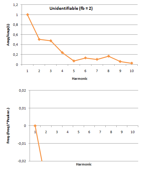
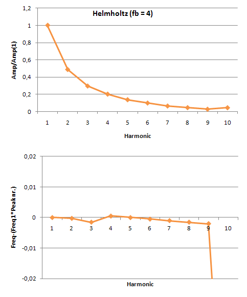
In order to do this we made amplitude plots in the frequency domain. This gives information about the frequencies at which high peaks appear and what their amplitudes are. We did this for the model as well as for our measurements. When we first analyzed the model, we seemed to be right in the fact that as the tone gets better, more peaks appear in the power spectrum. These peaks are not randomly spread out, but appear at harmonic frequencies. That is, at n-times the fundamental frequency with n being the number of the peak. This is also made visible in the figures below. These figures show the difference between the frequency that you would expect following this rule and the actual frequency that comes out of the model. For an unidentifiable tone, there are no harmonic tones on the expected frequencies, as the graph runs out of the figure. For a clear Helmholtz vibration however, the rule is satisfied for nine peaks. A second thing that becomes clear by analyzing the results from the model, is that the amplitude of every next peak decreases exponentially.

Figure 7: Amplitude ratio and frequency errors for an unidentifiable sound
Figure 8: Amplitude ratio and frequency errors for a Helmholtz vibration


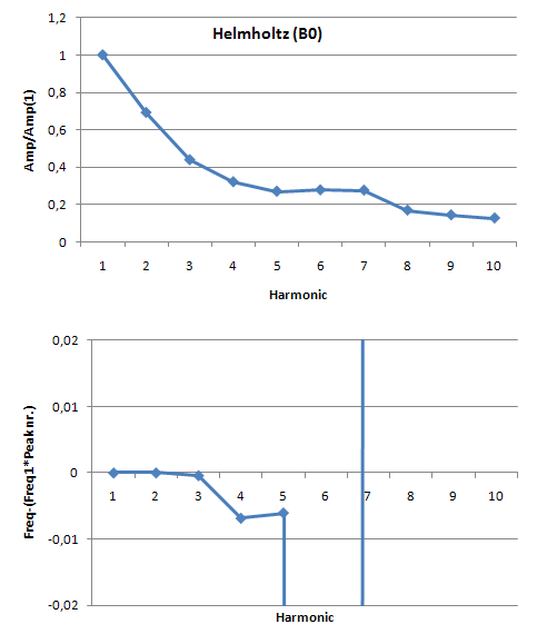
When we take a look at the measurements results, it becomes clear that these measurements are not as “clean” as the model. The same figures as for the model are also made for the measurements, as you can see below. The amplitude of the peaks does indeed decrease more or less exponentially as we would expect from the model. The number of peaks that appear at the expected frequency however, is only three for a vibration that sounded like a clear Helmholtz vibration to us. This can be explained by the fact that these measurements are done using a piezo element and the string vibrates along this element instead of perpendicular to it, which gives another signal. This problem is going to be solved however, because in the meantime experiments have proofed that the signal gets better when the string vibrates perpendicular, like it will on our prototype.

Figure 9: Amplitude ratio and frequency errors for measured Helmholtz sound

So, we seemed to be right in the fact that a vibration being Helmholtz has something to do with the frequencies at which harmonic peaks appear and the amplitude of that peaks compared to that of the fundamental frequency. There is only one important thing that makes this method of quantifying the signal irrelevant for our prototype control system. The point is that for this method a Fourier transformation needs to be done in the control unit in order to detect what the quality of the signal is. The problem is, that a Fourier transformation cannot be done instantaneously but only when enough information about the vibration is gathered. A simple rule tells that the resolution of the transformation equals 1/(sample time). In our case, where quality of the sound depends strongly on the exact frequencies where peaks appear, we should have a resolution in the frequency domain of at least 1 Hz. This means that the sample time for every transformation needs to be about a second, while the vibration needs to be adapted in several milliseconds up to several hundreds of seconds at most. So, this method is simply never going to satisfy our requirements. However, there is another way to perform this method, being in the time domain. When we take a look at the sawtooth like waveform of a Helmholtz vibration, we can already in the time domain draw some conclusions regarding to the quality of the vibration. The reason for this is that the harmonic peaks in the time domain, with their decreasing amplitudes, and the saw-toothed waveform in the time domain are strongly related to each other. A saw-toothed waveform essentially is a set of harmonic sinuses with decreasing amplitudes, being sharper when more harmonic sinuses are present. Putting this in an equation leads to the following expression for the signal, consisting of n harmonics:

[math]\displaystyle{ f=\sum_{i=1}^{n}(1/n) sin(nt) }[/math]

So the fact that more harmonic peaks appear in the frequency domain, finds is origin in the fact that more harmonic sinuses occur in the time domain. Moreover, when we want to quantify the signal in the time domain on the same properties as we did in the frequency domain, we only have to assess the signal on its sharpness. To proof this theory, figure 10 shows how the shape of the signal changes as the number of harmonic sinuses is increased. This leads to a perfectly sharp saw tooth, when the number of harmonic sinuses goes to infinity.

Figure 10: Sawtooth signals for an increasing number of harmonics


So, the idea is that we quantify the signal on the sharpness of the sawtooth. In order to do this we adapted our model and added a possibility to generate a sawtooth that serves as a reference. The correlation between the signal and our auto-generated reference sawtooth will be used as the quantification. This method will reduce the sample time to the longest period in the signal, which is 1 devided by the lowest frequency present in the signal. In this case the lowest frequency is about 100 Hz, so the sample time is about 10 milliseconds. To find out whether the signal indeed can be quantified on its sharpness (and thuss number of harmonics), we did some experiments. In the Helmholtz region, we varied the bowing speed at a constant bowing force and varied the bowing force at a constant speed. For all these simulations the correlation is calculated and plotted in the figures below (figures 11 and 12). From these figures, it can easily be concluded that there is not an ideal combination of bowing speed and force. That is, there is not an optimum which gives the best Helmholtz vibration. This means that when the vibration is a so called Helmholtz vibration, the system cannot be controlled to a point at which the correlation is highest. That is why we choose to make a lookup table with combinations of bowing speeds and forces that are in the Helmholtz region. The control unit then only needs to identify the fundamental frequency and lookup the right settings for the bowing speed and force. This gives great advantages regarding to adaptation time, because the controlling time now reduces to one sample time.

Figure 11: Correlation for varying bowing speeds
Figure 12: Correlation for varying bowing forces

Controller concept

The process described above, brought us to a controller design for the prototype. This controller makes use of a look-up table. This look-up table contains all the pre-defined values for bowing speed and force. By determining the fundamental frequency of the signal, the controller "knows" which fret is played and therefor what values for bowing speed and force are required. To make sure that the bowing speed indeed equals the value from the look-up table (also under varying bowing force) the engine speed is measured using an encoder and looped back to the controller. For the bowing force this does not seem to be neccesary, since the bowing force does not depend on the bowing speed.