Embedded Motion Control 2014 Group 12: Difference between revisions
| (58 intermediate revisions by 4 users not shown) | |||
| Line 1: | Line 1: | ||
==Introduction== | ==Introduction== | ||
| Line 214: | Line 213: | ||
</center> | </center> | ||
<br> | <br> | ||
==Line Detection == | |||
When regarding the designed software from the corridor competition, it became apparent that simply reading out the laser range data and comparing it against a set of reference values to determine the current situation was not really a robust solution. | |||
A better alternative would be to recognize lines surrounding PICO, instead of data points, and use this information to evaluate the situation. | |||
When investigating existing solution to this problem, the Hough transform came along quite frequently. | |||
However, this involves discretizing and memorizing a large number of points, which seemes wasteful for the specific problem faced by Pico. | |||
Instead of, say, an image, for which the Hough transform may very well be the best solution, Pico has to analyze a point cloud of subsequent points. | |||
So, a more natural method of line detection was chosen. | |||
Pico will start, for instance Line 1, by calculating the line between two subsequent points and representing this line with the vector through the origin, perpencidular to that line. | |||
Memorizing this line, the next two points are evaluated and if the line between these points matches the first line, the point is added to Line 1 and the next two points are compared to the first line. | |||
This is the basic idea behind the line detection algorithm, but several steps are taken to make it more robust. | |||
First of all, a gap tolerance is introduced which means that if a few lines do not match the reference line, but after that they match again, these few mismatching lines are still added. | |||
This is called a gap tolerance because it will filter gaps in the wall out of the lines. | |||
Next, a minimum length is introduced, which which makes sure that no lines of three or four lines are formed. | |||
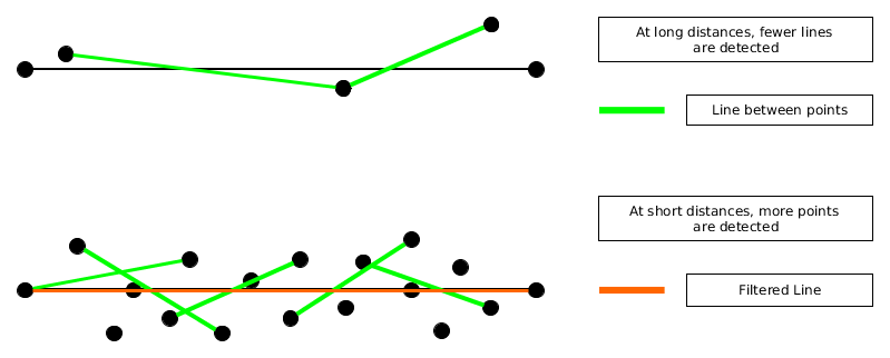
After closer inspection, the point cloud appeared to contain noise, which made determining the exact direction of the line difficult, see Figure. | |||
To overcome this problem, a very primitive low-pass filtering is applied by calculating the lines not between adjecent points, but between points further apart. | |||
However, this filtering made the accurate detection of corners more difficult and at greater distance, it was no longer as relevant. | |||
Therefore, the number of elements between the two points used, was made adaptive to the point being investigated. | |||
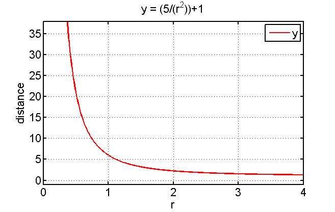
A tunable parameter, in this example taken 5, is divided by the radial distance to the point being investigated squared and one is added to make sure that even at great distance, the line will at least be calculated between adjecent points. | |||
[[File:EMC12_Graph.jpg]] | |||
[[File:EMC12_Line_point.png | If there are enough points at close distance, the algorithm will draw a line between the points. With enough lines, the data is filtered such that finally only the true line (colored in black) is recognized. This is depicted as the orange line. ]] | |||
Once the lines start to fundamentally mismatch, exceeding the gap tolerance, the algorithm returns to the last known line that matched, calls the starting point of this line the end point of Line 1 and names the end point of this line the starting point of Line 2. | |||
Any points lying between these points are discarded and from the starting point of Line 2 on, the cycle repeats. | |||
This method sometimes causes problems because of the way the lines are represented. | |||
The line through the origin, perpendicular to the line in question is represented in polar coordinates, but instead of <math>\theta \isin [-\pi,\pi]</math> and <math>r \isin [0,\infin]</math>, the range of <math>\theta \isin [0,\pi]</math> and <math>r \isin [-\infin, \infin]</math> is used. | |||
This means that lines just about straight ahead of Pico can either have a <math>\theta \approx 0 \or \pi</math>, depending on the direction of the deviation. | |||
To prevent this from breaking up a line, a second filtering is done, where this mismatch is corrected, to make sure that all lines that are in each others extension, are coupled. | |||
==World Model == | ==World Model == | ||
| Line 234: | Line 267: | ||
This was designed, and worked, for the strategy of driving through corners outside the measurement loop. | This was designed, and worked, for the strategy of driving through corners outside the measurement loop. | ||
When the choice was made to | When the choice was made to continuously measure, even in a corner, the world model was too rigid to handle all the adaptive movements involved and was not used. | ||
==Situation evaluation == | |||
The situation evaluation has been built in such a way that it fully profits from the built line detection algorithm. In order to be able to send a command to the situation act function several steps have been taken: | |||
* The character, or type, of the lines found by the line detection algorithm. | |||
* The intersections between the found lines. | |||
* Determine situation from unique combination of found lines and intersections. | |||
First of all the types of all the lines have to be determined, and in order to do this three line types have been defined: lines to the right of Pico (type 1), lines to the left of Pico (type 2) and horizontal lines (type 3). The character of these lines can be determined by the matching coordinates in the (r,<math>\theta</math>) space: a line to the right has a negative r coordinate and <math>\theta = 180^{\circ} \pm \delta</math>, with <math>\delta</math> as tolerance on the angle (in this case), while a line to the left has the same value for <math>\theta</math>, but a positive value for r. A horizontal line has no constraint on the sign of r (since it can both positive and negative), but <math>\theta=0^{\circ} \pm \delta</math>. | |||
This provides a robust detection of the relevant lines, because if a faulty diagonal is found (e.g. due to ghost points) the algorithm will not take it into account. Since no diagonal lines are present in the maze, and we assume that no lines will have a deviation of more than <math>\delta</math> w.r.t. to the ‘correct’ right angles. | |||
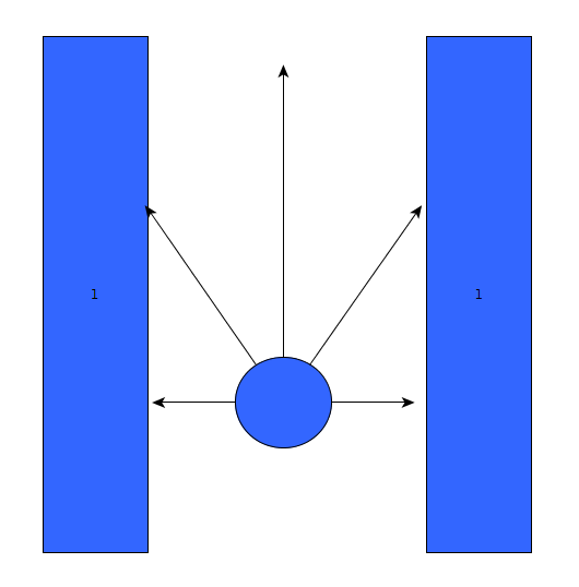
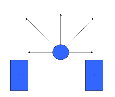
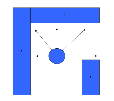
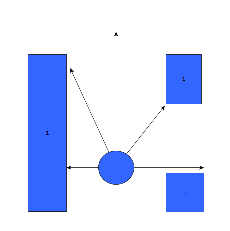
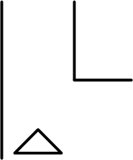
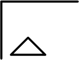
The second step in the algorithm is the determination of the intersections between all the lines. Four types of intersections have been defined: an open intersection (see Figure 1) between a line of type 1 and a line of type 3, an open intersection between a line of type 2 and a line of type 3, a closed intersection (see Figure 2) between lines of type 1 and 3 and a closed intersection between lines of type 2 and 3. | |||
Using these obtained parameters to determine the position of Pico in the maze is the last step of the algorithm: every situation Pico might encounter in a maze can be described by a unique combination of lines and intersections (e.g. corridor: >1 of type 1, > 1 of type 2, none of type 3, no intersections). This unique combination leads to a situation number (which is a ‘name’ for the found situation), which can then be sent to the situation act algorithm. | |||
<table> | |||
<tr> | |||
<td>[[File:Emc12_fig_1.png|thumb|center|100px|figure 1]]</td> | |||
<td>[[File:Emc12_fig_2.png|thumb|center|750px|figure 2]]</td> | |||
</tr> | |||
</table> | |||
==Movement== | ==Movement== | ||
| Line 254: | Line 308: | ||
Using some algebra, the distance to both walls perpendicular to the driving direction is found and used to strave to the centre of the corridor. | Using some algebra, the distance to both walls perpendicular to the driving direction is found and used to strave to the centre of the corridor. | ||
Averiging the angles under which the walls stand with respect to Pico allows for an adaptive rotational speed, aligning Pico . | Averiging the angles under which the walls stand with respect to Pico allows for an adaptive rotational speed, aligning Pico . | ||
Calling the straving velocity <math>v_y</math> and the rotational velocity <math>v_z</math>, the formulae used are: | |||
<math>v_y = \frac{r_l}{\cos(\theta_l)} + \frac{r_r}{\cos(\theta_r)} </math> | |||
<math>v_z = \frac{\theta_l + \theta_r - \pi}{2} </math> | |||
Please note that <math>r_r</math> is always negative, so this formula boils down to taking the difference in distance to the wall as a velocity. | |||
After bounding these values, the remaining linear velocity is disctributed to the forward velocity. | |||
The corridor can navigate skewed walls up to an angle of 30 degrees offset. | |||
===Dead end=== | |||
Once a dead end is detected, Pico exits the measuring loop and rotates more than 150 degrees. | |||
This is not a very clean solution, but it can never cause Pico to hit a wall since only a rotation is executed. | |||
The worst thing about this solution is when, for whatever reason, a false dead end is detected, which should cause Pico to exit at the entrance. | |||
===Corner=== | |||
The corner is taken in two parts. | |||
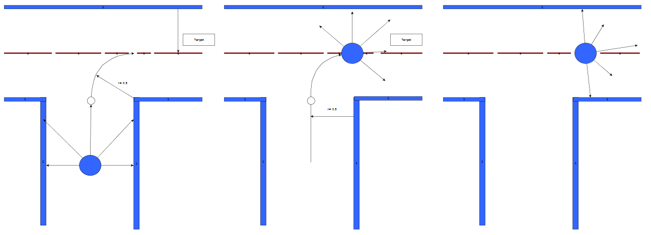
First, Pico follows the trajectory, as seen in the Figure. | |||
In the straight part of this movement, Pico drives at a fixed distance of 0.5 metre from the wall he will steer towards, but does not align. | |||
The method used, neutralizes the influence of the angle of Pico and makes sure the path he follows is always perpendicular to the wall he faces in the corner. | |||
Once Pico is 0.5 metre from the target line, he starts to combine forward velocity with a strave to travel an arc with a fixed radius of 0.5 metre. | |||
Once Pico is within a certain tolerance of the desired line, he starts rotating at maximum velocity. | |||
This means that Pico will be between the two new walls by the time that the situation evaluator no longer recognizes the walls surrounding Pico properly i.e., Pico is at a 30 degree angle with the wall. | |||
To allow this rotation to happen simultaniously with the arc, the influence of the angle is neutralized in this part of the movement too. | |||
This starts the second phase of the turn. | |||
In this phase, the 30 degree gap between the situation evaluator recognizing a wall as horizontal or vertical is bridged. | |||
Pico simply searches for the closest line and attempts to align with it's orientation. | |||
This will in practice never happen because the situation evaluator will recognize the new situation before full alignment is achieved. | |||
[[File:EMC12 Movement.png]] | |||
===Safety=== | |||
If the laser range finder finds any point within 30 cm of Pico, the situation evaluator is overwritten and the safety routine is executed. | |||
This routine simply causes Pico to move as fast as possible from the infringing point. | |||
==Fail Safe == | |||
In the current script, it is assumed that the situation can always be correctly evaluated. However, if for whatever reason the situation is not recognized, Pico would return a situation 0 ("Situation not recognized") and stop moving. This is most likely to happen when moving through a T-junction or a corridor, since their are many lines that can be recognized (both from corridor imperfections as well as other nearby crossings/coreners/T-junctions). This results in a set of criteria for the fail safe. It should: | |||
* Avoid walls (whatever the cost) | |||
* Continue the initiated movement | |||
* Or keep on driving/moving forward. | |||
For this, a simple wall "avoider" is build based on the principles of the script of the corridor challange. The idea is that Pico will always move forward and measure the distances around him. If there is a wall near by (within 40 cm), Pico will turn away from this wall (wall to the left: clockwise, to the right: counterclockwise) and then continue driving forward . If Pico finds himself driving straight at a wall he will stop and turn right. With these simple rules, Pico is able to finish all the movements that are initiated and then continue to drive. | |||
Ofcourse, there are a few downsides to this simple method. Since Pico turns away on de spot from nearby walls, it will lead to a bit of zigzagging in corridors. while this is not the most efficient way to move through a corridor, we assume that, by then, Pico has sucesfully recognized the situation and | |||
Another problem is a possible deadlock. Because of the zigzagging, if there are two corners with a corridor between them (with a minimal length of 1.8 meters given a corridor of 1 meter), Pico can become stuck in an loop. We assume however that Pico by then has already recognized the situation succesfully. This assumption is backed up by both simulations and experiments. | |||
==Arrow Recognition== | ==Arrow Recognition== | ||
| Line 312: | Line 380: | ||
===Dilate and Erode the Picture=== | ===Dilate and Erode the Picture=== | ||
The third step is to dilate and then erode the acquired HSV threshold image. | The third step is to dilate and then erode the acquired HSV threshold image. Dilate en erode both scan the image and place a box around the white or black pixels respectively and then fill the surrounding pixels with the same colour. A more formal definition about the function and their respective workings is given here [http://docs.opencv.org/doc/tutorials/imgproc/erosion_dilatation/erosion_dilatation.html]. The goal of first dilating (cv::dilate) is to fill up the contours, such that the relative contours (such as that of the arrow) can be detected more easily by other functions. After dilation, the image is eroded. The function, cv::erode, acts as a filter, and removes some of the noise from the image. | ||
===Blurring Image=== | ===Blurring Image=== | ||
| Line 406: | Line 473: | ||
The first step is to load the image and convert it to a binary (black/white) image using cv::cvtColor and cv::treshold. There is used an inverted tresholding (white lines, black background). | The first step is to load the image and convert it to a binary (black/white) image using cv::cvtColor and cv::treshold. There is used an inverted tresholding (white lines, black background). | ||
From this image, a region of interest is determined and the original image is resized. The lines of this new image are then dilated using cv::dilate to remove imperfections. Other options might be to use something like Canny edge detection or Hough transform, however the use of raw data with dilation works just as fine, due to the fact that the algorithm is robust for imperfections in the lines drawn in the image | From this image, a region of interest is determined and the original image is resized. The lines of this new image are then dilated using cv::dilate to remove imperfections. Other options might be to use something like Canny edge detection or Hough transform, however the use of raw data with dilation works just as fine, due to the fact that the algorithm is robust for imperfections in the lines drawn in the image. | ||
The walls are then detected by determining the contours (cv::findContours). There should be noted that lines that only belong to dead-ends are then removed. Lines enclosing a dead-end but that are still part of the final solution will be taken into account for the next step. The idea behind this is that a perfect maze only can have 2 walls in its trajectory. | The walls are then detected by determining the contours (cv::findContours). There should be noted that lines that only belong to dead-ends are then removed. Lines enclosing a dead-end but that are still part of the final solution will be taken into account for the next step. The idea behind this is that a perfect maze only can have 2 walls in its final, optimal trajectory. | ||
Next, these obtained contours are dilated and eroded. Ater this we can obtain the solution by substracting the eroded image from the dilated image (using cv:absdiff), resulting in the solution of the maze, which can ultimately be drawn into the original image of the maze. | Next, these obtained contours are dilated and eroded. Ater this we can obtain the solution by substracting the eroded image from the dilated image (using cv:absdiff), resulting in the solution of the maze, which can ultimately be drawn into the original image of the maze. | ||
| Line 422: | Line 489: | ||
<tr> | <tr> | ||
<td>[[File:1221.png|thumb|center|300px|Original image]] </td> | <td>[[File:1221.png|thumb|center|300px|Cropped Original image]] </td> | ||
<td>[[File: | <td>[[File:tresh1.png|thumb|center|300px|Treshold]]</td> | ||
<td>[[File: | <td>[[File:dilate2.png|thumb|center|300px|Dilate]] </td> | ||
</tr> | </tr> | ||
<tr> | <tr> | ||
<td>[[File: | <td>[[File:resize3.png|thumb|center|300px|Resized ROI]]</td> | ||
<td>[[File: | <td>[[File:dilate4.png|thumb|center|300px|Dilate ROI]]</td> | ||
<td>[[File: | <td>[[File:erode5.png|thumb|center|300px|Erode ROI]] </td> | ||
</tr> | </tr> | ||
<tr> | <tr> | ||
<td> | <td>[[File:abs6.png|thumb|center|300px|Absolute Difference]]</td> | ||
[[File: | <td>[[File:sol7.png|thumb|center|300px|Maze Solution]] </td> | ||
<td></td> | <td>[[File:sol78.png|thumb|center|300px|Additional solved Maze]] </td> | ||
<td></td> | |||
</tr> | </tr> | ||
</table> | </table> | ||
It can be seen that the algorithm correctly solves both given mazes. The algorithm is able to cope with diagonal mazes too, however this will connect the beginning and the end of the solution with eachother. Additional improvements could be the filtering of noise and ghost points. This successfull path can be implemented a second time PICO drives through the maze, to guarantee an optimal escape time from the maze. | |||
==Changelog | ==Changelog== | ||
<b>27-05</b><br> | <b>27-05</b><br> | ||
Created 3 line detection algorithms. | Created 3 line detection algorithms. | ||
| Line 464: | Line 531: | ||
<b>11-06</b><br> | <b>11-06</b><br> | ||
To be better able of coping with the uncertainty of the measurements and interpretation of the measurements by the line detection algorithm, a world model is added in three iterations. | To be better able of coping with the uncertainty of the measurements and interpretation of the measurements by the line detection algorithm, a world model is added in three iterations. | ||
The first iteration is a crude attempt, not using the line detection, but simply creating a discrete grid of Pico's surrounding and counting the number of measurements that fall within each grid point. After each measurement the previous measurement is partially forgotten. This works, but is memory consuming and inaccurate. | The first iteration is a crude attempt, not using the line detection, but simply creating a discrete grid of Pico's surrounding and counting the number of measurements that fall within each grid point. After each measurement the previous measurement is partially forgotten. This works, but is memory consuming and inaccurate. | ||
| Line 481: | Line 545: | ||
The state machine searches for starting points in the left regions and ending points in the right regions to determine if an event could take place. If another starting or ending point is near by, the found point indicates a fracture in the world model and not a possible corner and the event is rejected. | The state machine searches for starting points in the left regions and ending points in the right regions to determine if an event could take place. If another starting or ending point is near by, the found point indicates a fracture in the world model and not a possible corner and the event is rejected. | ||
Using the information from these four regions, all nine possibly states of Pico can be determined, as described in the corridor challenge. | Using the information from these four regions, all nine possibly states of Pico can be determined, as described in the corridor challenge. | ||
<b>18-06</b><br> | |||
During a meeting with the tutor, the idea to let Pico drive around corners without measuring the environment was concluded to lack robustness. | |||
Although the code in accordance with this philosphy was nearly finished, the choice was made to try and alter existing code to let Pico stay aware of his environment throughout all movements. | |||
The situation evaluation code, which had been pretty straight forward up untill now, had to be made significanlty more versatile to be able to recognize all situations and act consistently on it. | |||
Instead of searching in regions of interest, it switched to counting horizontal lines and lines to the left or right. | |||
Combining this with information on connections between these lines (corners) results in the recognizing of situations. | |||
The world model was discarded because one faulty measurement could no longer bring Pico in a dangerous position. | |||
Eventually, the choice was made to split in the cornering in two parts, also to simplify for the situation evaluator. | |||
The situation evaluator was given a tolerance of 30 degrees on both horizontal and vertical lines, which means that there is a 30 degree gap in which the situation evaluator does not take a line into account. | |||
In the case that no other situation could be distinguished, it is assumed that this is because all of the lines are outside the tolerance and Pico is told to align with the wall nearest by. | |||
This closest wall is most often the wall of the new corridor, although there are situations in which this is not the case. | |||
However suboptimal, it works in a lot of cases and because of the limited time, this solution was held and worked out. | |||
<b>19-06</b><br> | <b>19-06</b><br> | ||
Created a fail safe algorithm that ensures that Pico can continue to move along it's previous route even when the situation is not recognized and Pico | Created a fail safe algorithm that ensures that Pico can continue to move along it's previous route, even when the situation is not recognized and Pico does not any detect lines (basically: when everything goes wrong). | ||
==Experiments== | ==Experiments== | ||
| Line 506: | Line 584: | ||
<b>25-06-2014</b><br> | <b>25-06-2014</b><br> | ||
Created bagfiles to test future versions of mapping and the situation evaluator on real test cases. | |||
Also tested the corridor and safety movement functions. | |||
==Final Design== | ==Final Design== | ||
[[File:Emc12 overview.png | | [[File:Emc12 overview.png|center|thumb|700px|Final design that is implemented]] | ||
===Unique Selling Point | [[File:ArrowDetection_12.png|center|thumb|700px|link=http://youtu.be/NbFl-rrw76o| Youtube video displaying the final result. Notice the change in color at 0:26]] | ||
===Unique Selling Point=== | |||
* Home made line recognition and situation evaluator. | * Home made line recognition and situation evaluator. | ||
* Very robust Arrow Recognition | * Very robust Arrow Recognition | ||
* Map generation and | * Map generation and solving | ||
* | * Modular set up of the code: very easy to add and/or remove functions | ||
* Lightweight functions (especially line detection), leaving computational power for extra's | |||
* Only used nodes when timing was not critical, increasing robustness | |||
==Final result== | ==Final result== | ||
| Line 526: | Line 611: | ||
===What went right=== | ===What went right=== | ||
During the competition, Pico performed very well, driving the greatest distance without hitting any obstacle of any group. | |||
Other things that where succesful include: | |||
* Lines were succesfully recognized and situations were evaluated correctly | * Lines were succesfully recognized and situations were (mostly) evaluated correctly | ||
* A dead-end was recognized without actually going into it. | * A dead-end was recognized without actually going into it. | ||
* The alignment in the corridors went perfectly. | * The alignment in the corridors went perfectly. | ||
| Line 540: | Line 626: | ||
* Crossings | * Crossings | ||
The first crossing went as expected, Pico tried to take the first right corner, but noted it was a dead end end turned 180 degrees to continue his journey (recognizing the other dead-end on his right side). However, in the second crossing, due to unkown reasons, Pico | The first crossing went as expected, Pico tried to take the first right corner, but noted it was a dead end end turned 180 degrees to continue his journey (recognizing the other dead-end on his right side). However, in the second crossing, due to unkown reasons, Pico thought he was in a dead end and turned back again. Pico then drove on and recognized a dead end, which set him back on the proper route again. This time however; he did evaluate the situation correctly and turned right (as he should) at the appropriate time. We assume this loop occurred because a line was missed or not recognized in time. Since this behaviour was not observed in the simulation, it would be worthwhile to recreate this situation and test it in further experiments. | ||
* Alignment in the T-junction with arrow | * Alignment in the T-junction with arrow | ||
| Line 547: | Line 633: | ||
The last two situations could have been prevented with more time for testing and a bit of tuning of some parameters (especially the sleeptime of 0.05 seconds, increasing it could drastically alter the behaviour). | The last two situations could have been prevented with more time for testing and a bit of tuning of some parameters (especially the sleeptime of 0.05 seconds, increasing it could drastically alter the behaviour). | ||
===Evaluation=== | |||
Because of the late and abrupt change in strategy, many functions where made and simulated but never were used on Pico; and the ones that where used were insufficiently tested. | |||
This might have been avoided with better communication, a recurring theme in group work. | |||
Another problem was that the amount of work was distributed rather unevenly over the time, which suggests that the planning was perhaps too vague and we should have been more rigid in setting our goals. | |||
===Recommendations | ===Recommendations=== | ||
To improve the current code, most can be gained by making an (even more) intelligent situation evaluator, one that does not necessarily need to to know if a certain combination of lines and corners is a corner or a T-junction, but interprets the situation more humanlike and therefore, hopefully, more flexible. | |||
This proved too difficult to conceptualize in the last week, but it is a very interesting topic that might be further investigated. | |||
Another improvement would be to include some sort of memory in the situation evaluator so it doesn't need to deduce from the current information that it is trying to complete a corner, but can simply rely on the memorized value. This would add value to the current program, and it would not be hard to implement. | |||
Some of the search algorithms, such as in the corridor code where the wall on the right and on the left are searched for or the aligning, second part of the corner, could be made more robust by adding some extra checks whether or not the line found is the line that was searched for. | |||
While our strategy was to evaluate each situation through the use of line recognition and pre-programmed situations, it would be better if all this could be avoided. For that, an entirely different concept is required which would work in a very different way. An optimal solution would allow Pico to drive trough any maze without any constrains on the situations he could encounter (thereby also allowing for curved walls, obstacles in the middle of the path, etc.) and would be (almost) independent of tuning. | |||
There are two such concepts that posses these properties: (1) The map generation with Dijkstra's Algorithm for path finding and (2) The Repulsive Force Field. Off course, both have their merits and disadvantages, and there exists no perfect method, but these are the concepts we would definitely try next. | |||
==A word of thanks== | |||
Finally, we would like to thank our tutor Yanick Douven for his help and guidance during the project. We learned a lot about designing software from him as well as all the problems and situations one has to think of if one wants the code to become even slightly robust. | |||
Latest revision as of 20:23, 2 July 2014
Introduction
Members of group 12
| Groupmembers (email all) | ||
| Name: | Student id: | Email: |
| Anthom van Rijn | 0737682 | e-mail Anthom |
| Jan Donkers | 0724801 | e-mail Jan |
| Jeroen Willems | 0755833 | e-mail Jeroen |
| Karel Drenth | 0863408 | e-mail Karel |
Corridor Challenge
The goal of the corridor challenge is to make pico drive autonomously trhough a corridor, recognize a T-junction successfully, and have it take the appropriate corner.
Planning
Week 1
- First Lecture
Week 2
- C++ tutorials
- ROS tutorials
- SVN tutorials
- Run the first test on pico (safe_drive.cpp) to get some hands-on experience.
Week 3
- Start the actual coding, based on the safe_drive.cpp file. Paying special attention to robustness and exceptions.
- Have pico recognize situations (corridor, corner, t-junction,dead-end, etc.) and act accordingly
- Have the script succesfully run in simulation
Week 4
- Fine tuning of script
- Corridor Competition
Software Architecture
Initially, the choice was made to forgo the notion of speed and first create a robust algorithm that would successfully recognize a situation, using only the laser data, and take the appropriate action. The situations that should be recognized are depicted in table below. In this case, it's assumed that all junction/corners are right handed, although it works equally for left handed situations.
Situation recognition
Goal: to successfully recognize a situation and take the corresponding action.
Robustness
As can be seen, it is important to calibrate the ranges of the laser data to make sure that the situation is evaluated correctly. If this is done wrong, the situation might be evaluated incorrectly and PICO might come to a halt (due to a hard constraint) and be unable to continue. To illustrate this, below are some possible pitfalls and the solution.
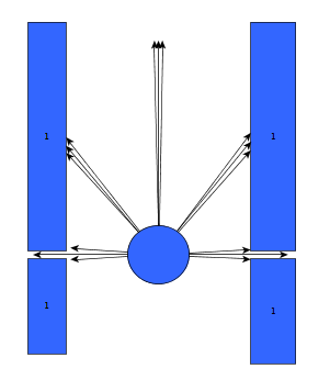
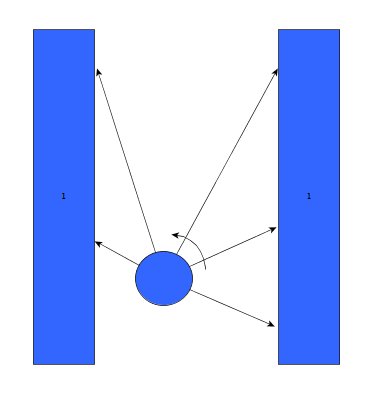
As can be seen in the figures above, it is quite difficult to use only some of the laser data to figure out the situations and still be robust for all the things that can be encountered. While the presented situations are good enough for a simple corridor challenge, other alternatives should be considered when regarding finding the way through a maze, for the reliance on proper tuning isn't good practice when writing code. Another disadvantage is that with the current set-up, only pre-programmed situations can be successfully recognized. While there are only a limited number of situations that can be encountered in the maze challenge, the code is not able to with with things like curved walls.
Experiments
09-05
Tested the provided safe_drive file, making small alteration to see the effects on Pico. Tested how hard constrains are handled and some different safety protocols.
13-05
Tried, and failed, to run corridor_challenge_v2 due to numerous bugs in the script (most importantly: stuck in situation zero, unsure what to do). Received help from tutor regarding tips and tricks regarding Qt creator for debugging, building/making C++ in ROS and running simulations. Information was used to create a "how to start: Pico" tutorial. Remainder of time spent on bugfixing.
Change log
09-05
Created scipt corridor_challenge.cpp with basic siteval to recognize conditions
13-05
Testing corridor_challenge on Pico.
With new input from experiments: updated the corridor_challenge.cpp to corridor_challenge_v2.cpp.
Brought the function sit-eval withing the callback loop for sensor messages. This way, the situation is evaluated and updated whenever new laser data is present. Some minor typo's. Added a situation that when things are to close (hard constraint) pico shuts down. After testing it was revealed that pico is stuck in condition 0 (does not know where he is).
15-05
- Revised corridor_challenge_v2.cpp -> renamed to corridorchallenge_v2.cpp and added some new functions:
- Extended laser 'vision' with left- and right diagonal view and updated amount of laser data used for each 'vision' vector.
- Extended the amount of possible situation PICO can be in to nine. Currently using:
- Corridor
- T-Junction (L+R)
- Crossing
- Corner (L+R)
- Dead End
- Exit
- Added a function that compares the left and right laser data and 'strafes' PICO to the middle using the y coordinate.
- Added an 'integrator'-like function that aligns the front vector of PICO to the walls of the corridor.
- Included front laser data to this function to ensure 'backup' when PICO comes too close to a wall.
- Added corresponding functions to new situations.
- Tweaked variables to ensure functioning simulations. (Allowance of some initial angle with reference to wall 'disturbance'). PICO is currently able to pass corridors, T-junctions and corners, for this however, the amount of possible situations PICO can be in is reduced for the sake of simplicity.
Final Design
The final design that was used was corridor_challenge_v2. It's goal was to use the laser data to recognize one of 9 conditions (ranging from freedom, corridor) and act in a preprogrammed way (outside of the loop) on how to handle these, and then turn on the loop again.
Result
Due to some unforeseen circumstances, corridorchallenge v3 failed to load on PICO. We resorted back to v2, which, while less robust, was still able to find the t-junction and act accordingly. The result was a first place in the "limited speed" category, with a time close to 20 seconds.
Maze Challenge
The goal of the Maze Challenge is to have PICO drive autonomously through a maze and successfully navigate itself towards the exit. There are three major assumptions
- (1) The Maze is two dimensional (all the walls, as well as the entrance and exits are on the ground floor level. There is no way to go either up or down).
- (2) Both the entrance and the exits are on the outer edge of the maze.
- (3) The maze does not change with time.
While these assumptions might seem redundant, they are of major importance when determining the strategy
Strategy
Because of the three assumptions earlier, there are two practical ways to solve the maze.
- Always go right. Assuming that the error and the entrance is indeed on the edge of the maze, a simple right wall follower would always find the exit. However, there is no guarantee that all the possible routes are explored, and hence it is not possible to generate the shortest route.
- Take every possible corner. While this can be very time consuming, using clever algorithms (see [1]) it can be assured that the maze it thoroughly explored and that, at the end of the run, an entire map is available which could be used to find the shortest route to the exit.
Here, a trade-off has to be made. The first strategy is pretty easy to implement, and although it is not the fastest way, it is very robust. Because of this robustness, this strategy is implemented first to assure PICO fins an exit. Then, if time allows, the second strategy will be attempted.
Planning
Week 5
- Group meeting discussing the new strategy to finish solve the maze challenge
- Start coding on the line detection script
- Begin with arrow detection
Week 6
- Debugging and finalizing the line detection script
- Starting with coding the function for map generation
- Making a with function to combine line detection with a situation evaluation
Week 7
- Finalizing arrow detection
- Combing arrow detection with the situation evaluation
- Building in a fail-safe
Week 8
- Finalizing script
- Debugging all the code
- Updating wiki
Software architecture / Road map
Line Detection
When regarding the designed software from the corridor competition, it became apparent that simply reading out the laser range data and comparing it against a set of reference values to determine the current situation was not really a robust solution. A better alternative would be to recognize lines surrounding PICO, instead of data points, and use this information to evaluate the situation.
When investigating existing solution to this problem, the Hough transform came along quite frequently. However, this involves discretizing and memorizing a large number of points, which seemes wasteful for the specific problem faced by Pico. Instead of, say, an image, for which the Hough transform may very well be the best solution, Pico has to analyze a point cloud of subsequent points. So, a more natural method of line detection was chosen. Pico will start, for instance Line 1, by calculating the line between two subsequent points and representing this line with the vector through the origin, perpencidular to that line. Memorizing this line, the next two points are evaluated and if the line between these points matches the first line, the point is added to Line 1 and the next two points are compared to the first line.
This is the basic idea behind the line detection algorithm, but several steps are taken to make it more robust. First of all, a gap tolerance is introduced which means that if a few lines do not match the reference line, but after that they match again, these few mismatching lines are still added. This is called a gap tolerance because it will filter gaps in the wall out of the lines. Next, a minimum length is introduced, which which makes sure that no lines of three or four lines are formed. After closer inspection, the point cloud appeared to contain noise, which made determining the exact direction of the line difficult, see Figure. To overcome this problem, a very primitive low-pass filtering is applied by calculating the lines not between adjecent points, but between points further apart. However, this filtering made the accurate detection of corners more difficult and at greater distance, it was no longer as relevant. Therefore, the number of elements between the two points used, was made adaptive to the point being investigated. A tunable parameter, in this example taken 5, is divided by the radial distance to the point being investigated squared and one is added to make sure that even at great distance, the line will at least be calculated between adjecent points.
Once the lines start to fundamentally mismatch, exceeding the gap tolerance, the algorithm returns to the last known line that matched, calls the starting point of this line the end point of Line 1 and names the end point of this line the starting point of Line 2. Any points lying between these points are discarded and from the starting point of Line 2 on, the cycle repeats.
This method sometimes causes problems because of the way the lines are represented. The line through the origin, perpendicular to the line in question is represented in polar coordinates, but instead of [math]\displaystyle{ \theta \isin [-\pi,\pi] }[/math] and [math]\displaystyle{ r \isin [0,\infin] }[/math], the range of [math]\displaystyle{ \theta \isin [0,\pi] }[/math] and [math]\displaystyle{ r \isin [-\infin, \infin] }[/math] is used. This means that lines just about straight ahead of Pico can either have a [math]\displaystyle{ \theta \approx 0 \or \pi }[/math], depending on the direction of the deviation. To prevent this from breaking up a line, a second filtering is done, where this mismatch is corrected, to make sure that all lines that are in each others extension, are coupled.
World Model
A way of making the perception of Pico more robust, is to allow him to remember what his environment looked like previously. This was done by making a world model, relative to the centre of Pico. If at one point several lines are detected and the next few moments all of these lines but one are detected over and over again, this one measurement should be forgotten. Also, if a line happens to be fractured, the world model should glue these pieces back together.
To achieve this, the world model algorithm compares the lines it receives from the new measurement to the ones it had stored in the world model. This is done by determining the direction of the line, then drawing a box around this line and finally determining if a start or end point falls within this box. If a match is found, the most likely coordinates of the starting point and ending point are calculated by averaging. If no match is found, the line is added to the world model. All lines in the world model also get a counter, which goes up every time a match is found for the line.
Updating this world model is done in two ways, every iteration, all lines in the world model lose a number of points and if there are no points left, the line is removed from the world model. This allows the world model to forget false readings. Secondly, the world model is updated based on the movement Pico will make. If Pico drives down a corridor, all lines a shifted back a little, if Pico makes a turn in a dead end all lines are flipped and if Pico takes a turn, the world model is cleared.
This was designed, and worked, for the strategy of driving through corners outside the measurement loop. When the choice was made to continuously measure, even in a corner, the world model was too rigid to handle all the adaptive movements involved and was not used.
Situation evaluation
The situation evaluation has been built in such a way that it fully profits from the built line detection algorithm. In order to be able to send a command to the situation act function several steps have been taken:
- The character, or type, of the lines found by the line detection algorithm.
- The intersections between the found lines.
- Determine situation from unique combination of found lines and intersections.
First of all the types of all the lines have to be determined, and in order to do this three line types have been defined: lines to the right of Pico (type 1), lines to the left of Pico (type 2) and horizontal lines (type 3). The character of these lines can be determined by the matching coordinates in the (r,[math]\displaystyle{ \theta }[/math]) space: a line to the right has a negative r coordinate and [math]\displaystyle{ \theta = 180^{\circ} \pm \delta }[/math], with [math]\displaystyle{ \delta }[/math] as tolerance on the angle (in this case), while a line to the left has the same value for [math]\displaystyle{ \theta }[/math], but a positive value for r. A horizontal line has no constraint on the sign of r (since it can both positive and negative), but [math]\displaystyle{ \theta=0^{\circ} \pm \delta }[/math].
This provides a robust detection of the relevant lines, because if a faulty diagonal is found (e.g. due to ghost points) the algorithm will not take it into account. Since no diagonal lines are present in the maze, and we assume that no lines will have a deviation of more than [math]\displaystyle{ \delta }[/math] w.r.t. to the ‘correct’ right angles.
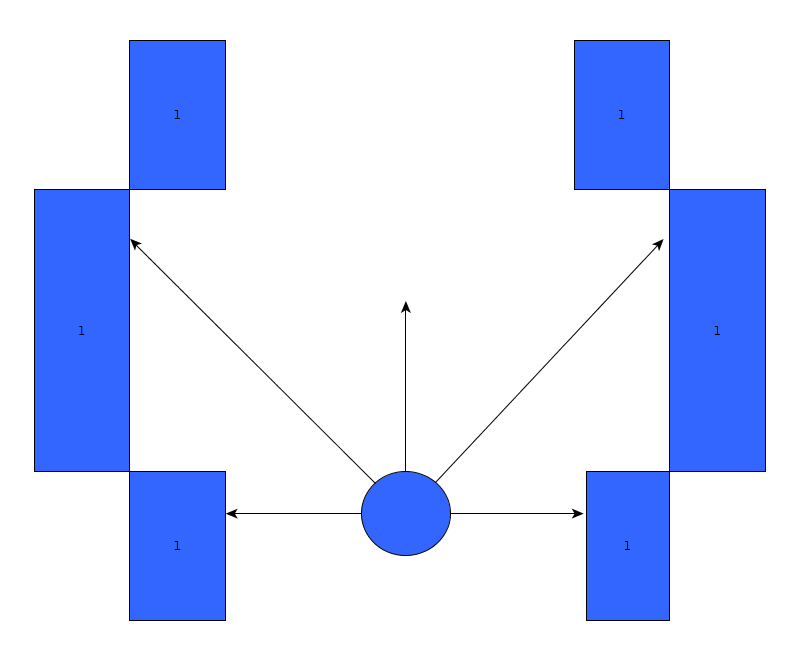
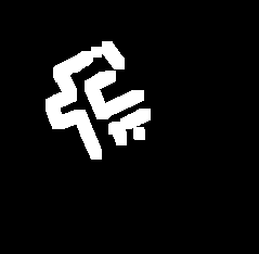
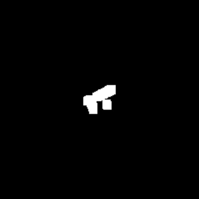
The second step in the algorithm is the determination of the intersections between all the lines. Four types of intersections have been defined: an open intersection (see Figure 1) between a line of type 1 and a line of type 3, an open intersection between a line of type 2 and a line of type 3, a closed intersection (see Figure 2) between lines of type 1 and 3 and a closed intersection between lines of type 2 and 3.
Using these obtained parameters to determine the position of Pico in the maze is the last step of the algorithm: every situation Pico might encounter in a maze can be described by a unique combination of lines and intersections (e.g. corridor: >1 of type 1, > 1 of type 2, none of type 3, no intersections). This unique combination leads to a situation number (which is a ‘name’ for the found situation), which can then be sent to the situation act algorithm.
 |
 |
Movement
There are three basic movements Pico needs to make and a security measure.
Corridor
When driving down a corridor, the goal is to stay centered and aligned with the walls. However, the walls are not necessarily parallel. First, two reference lines are searched. Since the laser range finder measures from right to left, the lines on the right will be at the start of the detected lines and the walls on the left at the end. So, a wall on the right is searched from start to end, a wall on the left is searched from end to start. This minimizes searching time, although this is most likely very small anyway.
The properties of the lines through the origin perpendicular to the wall left and right are retrieved. Using some algebra, the distance to both walls perpendicular to the driving direction is found and used to strave to the centre of the corridor. Averiging the angles under which the walls stand with respect to Pico allows for an adaptive rotational speed, aligning Pico . Calling the straving velocity [math]\displaystyle{ v_y }[/math] and the rotational velocity [math]\displaystyle{ v_z }[/math], the formulae used are:
[math]\displaystyle{ v_y = \frac{r_l}{\cos(\theta_l)} + \frac{r_r}{\cos(\theta_r)} }[/math]
[math]\displaystyle{ v_z = \frac{\theta_l + \theta_r - \pi}{2} }[/math]
Please note that [math]\displaystyle{ r_r }[/math] is always negative, so this formula boils down to taking the difference in distance to the wall as a velocity. After bounding these values, the remaining linear velocity is disctributed to the forward velocity. The corridor can navigate skewed walls up to an angle of 30 degrees offset.
Dead end
Once a dead end is detected, Pico exits the measuring loop and rotates more than 150 degrees. This is not a very clean solution, but it can never cause Pico to hit a wall since only a rotation is executed. The worst thing about this solution is when, for whatever reason, a false dead end is detected, which should cause Pico to exit at the entrance.
Corner
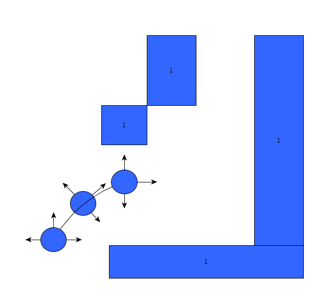
The corner is taken in two parts. First, Pico follows the trajectory, as seen in the Figure. In the straight part of this movement, Pico drives at a fixed distance of 0.5 metre from the wall he will steer towards, but does not align. The method used, neutralizes the influence of the angle of Pico and makes sure the path he follows is always perpendicular to the wall he faces in the corner. Once Pico is 0.5 metre from the target line, he starts to combine forward velocity with a strave to travel an arc with a fixed radius of 0.5 metre. Once Pico is within a certain tolerance of the desired line, he starts rotating at maximum velocity. This means that Pico will be between the two new walls by the time that the situation evaluator no longer recognizes the walls surrounding Pico properly i.e., Pico is at a 30 degree angle with the wall. To allow this rotation to happen simultaniously with the arc, the influence of the angle is neutralized in this part of the movement too. This starts the second phase of the turn.
In this phase, the 30 degree gap between the situation evaluator recognizing a wall as horizontal or vertical is bridged. Pico simply searches for the closest line and attempts to align with it's orientation. This will in practice never happen because the situation evaluator will recognize the new situation before full alignment is achieved.
Safety
If the laser range finder finds any point within 30 cm of Pico, the situation evaluator is overwritten and the safety routine is executed. This routine simply causes Pico to move as fast as possible from the infringing point.
Fail Safe
In the current script, it is assumed that the situation can always be correctly evaluated. However, if for whatever reason the situation is not recognized, Pico would return a situation 0 ("Situation not recognized") and stop moving. This is most likely to happen when moving through a T-junction or a corridor, since their are many lines that can be recognized (both from corridor imperfections as well as other nearby crossings/coreners/T-junctions). This results in a set of criteria for the fail safe. It should:
- Avoid walls (whatever the cost)
- Continue the initiated movement
- Or keep on driving/moving forward.
For this, a simple wall "avoider" is build based on the principles of the script of the corridor challange. The idea is that Pico will always move forward and measure the distances around him. If there is a wall near by (within 40 cm), Pico will turn away from this wall (wall to the left: clockwise, to the right: counterclockwise) and then continue driving forward . If Pico finds himself driving straight at a wall he will stop and turn right. With these simple rules, Pico is able to finish all the movements that are initiated and then continue to drive.
Ofcourse, there are a few downsides to this simple method. Since Pico turns away on de spot from nearby walls, it will lead to a bit of zigzagging in corridors. while this is not the most efficient way to move through a corridor, we assume that, by then, Pico has sucesfully recognized the situation and Another problem is a possible deadlock. Because of the zigzagging, if there are two corners with a corridor between them (with a minimal length of 1.8 meters given a corridor of 1 meter), Pico can become stuck in an loop. We assume however that Pico by then has already recognized the situation succesfully. This assumption is backed up by both simulations and experiments.
Arrow Recognition
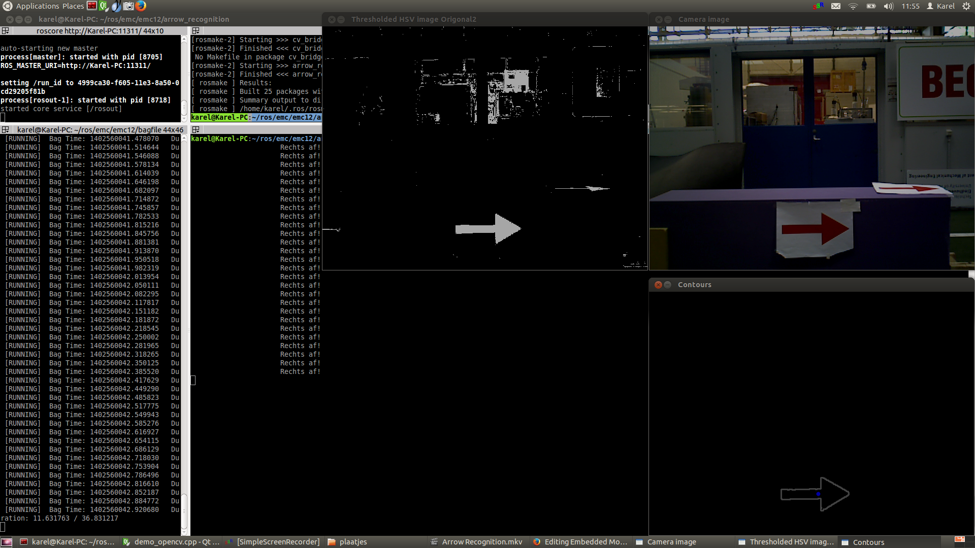
For the recognition of arrows in the maze, a node calld arrow_recognition is created. The node is subscribed to the function imageCallback, which receives the data of the image and then processes it (the functioning will be described below). It then sends a messages (the direction of the arrow) over the channel /maze/arrow. Every 0.05 seconds the node spins and the imageCallback is performed, resulting into a message being sent over the defined channel. For image processing the OpenCV toolbox is used.
ROS RGB to OpenCV RGB
The first step is to convert the ROS RGB image (acquired by ROS subscription to /pico/asusxtion/rgb/image_color) to an OpenCV image so that it can be processed using this toolbox.
OpenCV RGB to HSV
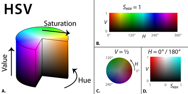
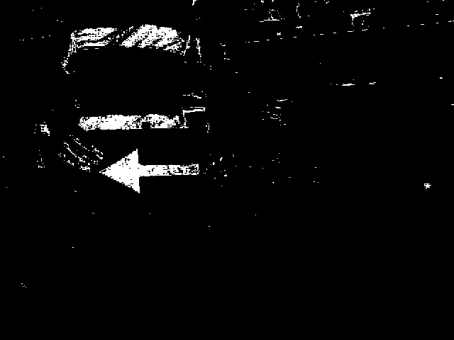
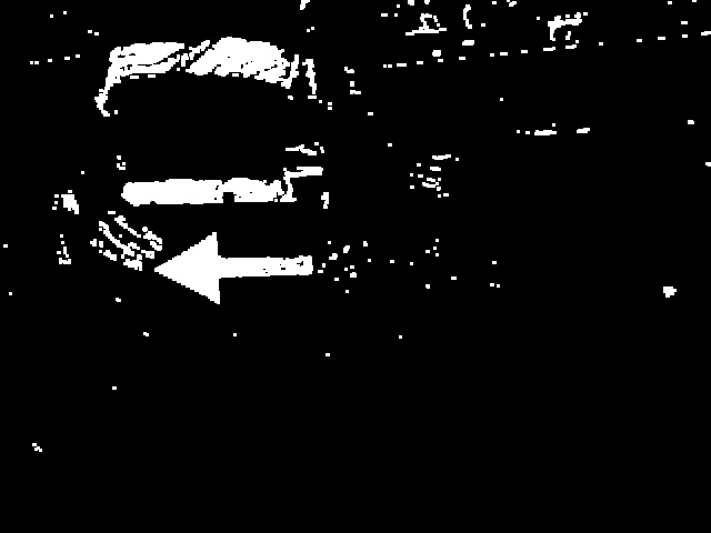
The second step is to convert the RGB image to HSV color space (Hue, Saturation, Value), using cv::cvtColor. This technique allows thresholding of the image so certain specific HSV values can be extracted from the image. This is done using the cv::inRange command, using a set of minimum and maximum values for Hue, Saturation and Value. These values are tuned iteratively by simulating pre-recorded bagfiles. Special care is taken that the range in which the colours are selected is larger then strictly necessary for robustness. This turned out to be necessary, since :
- The lightning conditions can vary wildly depending on the surroundings.
- The focus of the camera can change, resulting in a different set of colours (see the youtube video [2]around 00:23 seconds)
A clear disadvantage of a larger range offcourse is that a lot more points are detected and the image becomes noisier.
Dilate and Erode the Picture
The third step is to dilate and then erode the acquired HSV threshold image. Dilate en erode both scan the image and place a box around the white or black pixels respectively and then fill the surrounding pixels with the same colour. A more formal definition about the function and their respective workings is given here [3]. The goal of first dilating (cv::dilate) is to fill up the contours, such that the relative contours (such as that of the arrow) can be detected more easily by other functions. After dilation, the image is eroded. The function, cv::erode, acts as a filter, and removes some of the noise from the image.
Blurring Image
Using cv::blur and cv:equalizeHist, the image is smoothed and the intensity range is stretched out. This results into an image for which the edges are smoothend, which makes them easier to detect.
Canny Edge Detection
Now that several OpenCV functions have been used to modify the image, an edge detection function (cv::Canny) can be applied to extract a set of edges from the image. The function makes use of noise filtering, intensity gradients, suppression of pixels not belonging to the edge and hysteresis. [4]
Find Contours
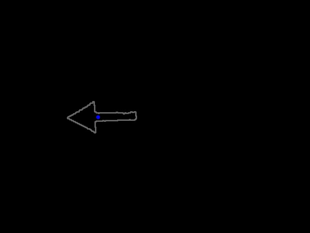
Now that the edges have been detected succesfully, we can start creating closed contours from these edges, using cv::findContours to detect and cv:drawContours to draw the detected contours.
Select arrow contour using constraints
Now that all the contours have been found successfully, the contour matching to the arrow has to back selected from the set of all contours identified. For this, a set of constraints is constructed, which are discussed below.
- Looping over all the contours found, using cv:boundingRect, rectangles will be fitted over all the contours and the (x,y) position of all the corners of these rectangles will be logged. The first constraint can now be applied: the length of the rectangle in x direction has to has to be bigger than 2.05 times that of the y direction and smaller than 2.35 times the y direction of the rectangle.
- Next, cv::approxPolyDP is used to approximate the areas of all the contours that are left. This area is called a. The next step is to use cv:convexHull, which creates a convex hull around all the contours, this area is called b. Since the arrow has a fixed shape, there excists a relation between a and b, which is always around 0.6.
- As a final selection criteria, only the the contours that have areas with more then 3000 or 2000 pixels for (a and b respectively) are taken in consideration. These values also dictate up to which distance you can successfully detect an arrow.
- Ultimately, the only contour passing this set of constraints is the desired contour of the arrow at a range of around 1.5 meter.
Determine arrow direction using mass moments
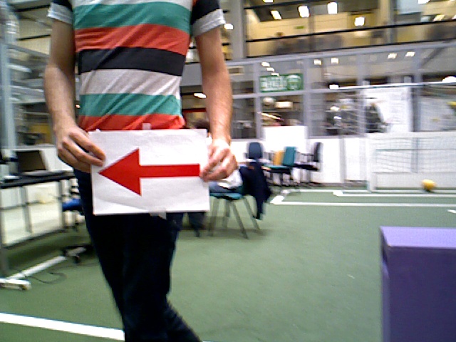
Once the arrow has been succesfully extracted from the image, it's direction has to be determined. For this, the arrows centre of mass (x,y) is calculated using the so called Hue-moments (cv:moments) and is depicted in the image as a blue dot. These coordinates (x,y) will be compared with the middle of the bounded rectangle, created one step earlier. If the mass middle is more to the left than the middle of the bounded rectangle, the arrow is pointing towards to the left! Vice versa of course for an arrow pointing to the right.
Memory
The created algorithm is now able to select the arrow contour and determine the direction. The last step is to define the message that has to be published, which is either a 1 (arrow pointing left detected), a 0 (no arrow detected) or a -1 (arrow pointing right detected). For robust selection, an exponential moving average is used. For this, a rolling average variable and two weighting factors \alpha and \beta are defined. If a direction is detected, this rolling average variable will be updated via a convex combination of the detected value and the memory of the rolling_avg variable.
rolling_avg = (alpha*detected_direction)+(1.0-alpha)*rolling_avg
- where: detected_direction = 1 (if left) and detected_direction = -1 (if right)
- When no direction is detected, the following formula is applied:
rolling_avg = (1.0-beta)*rolling_avg;
This will result into the exponential moving average that goes towards 0. This means that when no arrow is detected for a certain amount of time, the command no arrow will be correctly published and if a single wrong measurement is taken, it has no influence. The algorithm has been tested on several bagfiles and has proven to work 100% of the time.
Overview process
Below pictures are shown describing the entire process. There should be noted that probably the HSV values can be set stricter to select even less contours, although some room is given to ensure robustness for variations of the light level in the area PICO will drive.
| Corridor challenge | ||
 |
 |
 |
 |
 |
 |
 |
 |
Map Generation
After Pico has succesfully recorded all transform and laser scan data, a 2D map can be created. For this, the function gmapping will be used. [5] Gmapping uses the odometry sensor (estimation of position and orientation) and the laser scanner (create a more accurate estimate) to estimate the map.
This package is able to generate a live map of the incoming data of Pico or to playback from a bagfile. Ultimately, the generated map can be saved using map_server map_saver.
The gmapping algorithm makes use of the simultaneous localization and mapping procedure (SLAM). This approach uses a particle filter which each particle carries an individual map of the environment. [6] The nice thing of this algorithm is that a map is created of which the orientation stays the same the entire time and is thus able to take rotation of Pico into account. It is also possible to draw the trajectory driven by Pico inside this generated map. Live-mapping is then able to detect that Pico has already been at a certain corridor once, so that Pico does not have to enter that corridor again after a dead end is detected. Offline-map recognition is able to detect the optimal trajectory through the maze, which will be discussed in the next paragaph.
There has to be noted that the displayed map is not perfect, this due to imperfections caused by real world implementation, such as wheel slip. If Pico drives a second time through the imperfect area, the gmapping algorithm is able to compensate for this imperfection.
Determination of optimal path
After an image of the entire maze has been generated, an algorithm determining the optimal solution can be applied. This algorithm will be explained in this paragraph. We will make use of the OpenCV image processing toolbox.
The first step is to load the image and convert it to a binary (black/white) image using cv::cvtColor and cv::treshold. There is used an inverted tresholding (white lines, black background).
From this image, a region of interest is determined and the original image is resized. The lines of this new image are then dilated using cv::dilate to remove imperfections. Other options might be to use something like Canny edge detection or Hough transform, however the use of raw data with dilation works just as fine, due to the fact that the algorithm is robust for imperfections in the lines drawn in the image.
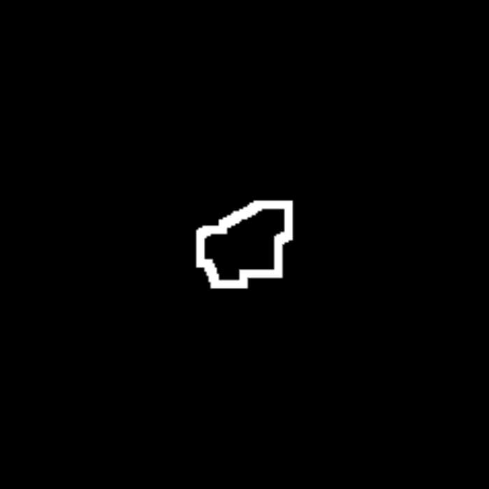
The walls are then detected by determining the contours (cv::findContours). There should be noted that lines that only belong to dead-ends are then removed. Lines enclosing a dead-end but that are still part of the final solution will be taken into account for the next step. The idea behind this is that a perfect maze only can have 2 walls in its final, optimal trajectory.
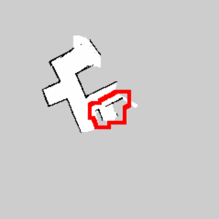
Next, these obtained contours are dilated and eroded. Ater this we can obtain the solution by substracting the eroded image from the dilated image (using cv:absdiff), resulting in the solution of the maze, which can ultimately be drawn into the original image of the maze.
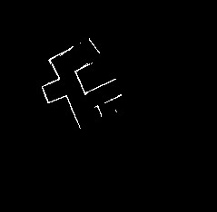
From the following pictures (map created from bagfile), it can be seen that the algorithm is robust for imperfections in the lines. This, due to the fact that the algorithm is based on pixel points in the image, as long as pixels are connected (improved by dilation of the image) this algorithm is able to function properly. Thus, robustness for gaps is guaranteed as long as the amount of pixels dilated is high enough.
| Corridor challenge | ||
 |
 |
 |
 |
 |
 |
 |
 |
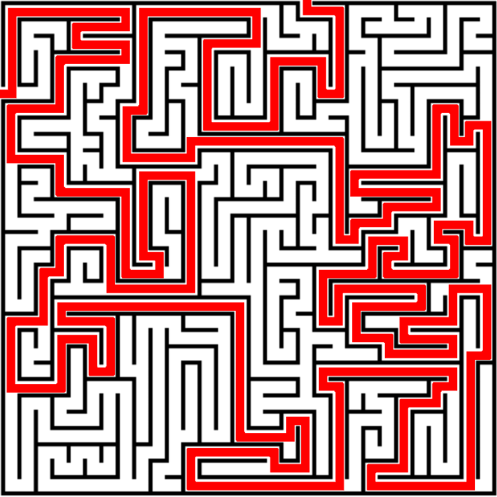 |
It can be seen that the algorithm correctly solves both given mazes. The algorithm is able to cope with diagonal mazes too, however this will connect the beginning and the end of the solution with eachother. Additional improvements could be the filtering of noise and ghost points. This successfull path can be implemented a second time PICO drives through the maze, to guarantee an optimal escape time from the maze.
Changelog
27-05
Created 3 line detection algorithms.
First algorithm calculates the line between two subsequent points in r-theta space (Hough transform) and compares these values with the line between the next two points. If the next line is, within tolerances, similar to the first line, its point is added to the line and the next line is compared to the first line. To allow for gaps in the walls or incorrect measurements, a certain number of lines is allowed to be misaligned with the reference line if another line follows that does have the correct orientation. If this number of 'gap-lines' is exceeded, the algorithm returns to the first point that misaligned with the reference line and a new line is started from there. If the number of elements contained in the line is shorter than a certain value, the line is discarded as irrelevant.
This algorithm proved unreliable and produced many interrupted lines.
In the second version the found lines are once more represented in r-theta coordinates and once again compared to each other in an attempt to sew interupted lines together. This proved not as effective as hoped.
A start was made with the third version, which functiosn similarly to the first version but compares lines between two points that are 10 measrements away. More accurately described in the update of 06 06.
06-06
After some investigation, it turned out that the measurement was relatively noisy, especially close to the robot. The third version is very similar to the first version, but uses two measurement points, a variable number of elements apart. This results in a low pass filtering of the laser data. The higher the number of elements, the smoother the line becomes, but the harder corners are to accurately detect.
Another difficulty is that one line may now span acros an opening, such as a corridor, and in some cases it recognizes a diagonal line that does not exist. To prevent this, a constraint is added that does not allow the two points that are considered to be further apart than a certain threshold.
This algorithm has a lot of parameters to tune, 6, but shows good results.
11-06
To be better able of coping with the uncertainty of the measurements and interpretation of the measurements by the line detection algorithm, a world model is added in three iterations.
The first iteration is a crude attempt, not using the line detection, but simply creating a discrete grid of Pico's surrounding and counting the number of measurements that fall within each grid point. After each measurement the previous measurement is partially forgotten. This works, but is memory consuming and inaccurate.
The second iteration is based on the first observation of Pico. If the line detection finds a line with similar orientation and that ends or starts within a certain tolerance of a line in the first observation of Pico, a number of points is added to that line. After each measurement, each line also loses a number of points and when the line has no points left, it is removed from the world model. If no match is found for a line within the world model, the new line is added to the world model. To compensate for the movement of Pico, all lines are moved a little if the robot moves forward, all lines are turned around if the robot turns in a dead end and if Pico takes a corner, it forgets the world model.
The third iteration also includes a section that updates the lines in the world model. If the starting or ending point of a measured line is close to the start or end point of a line in the world model, the location of that point is averaged between the two. If a measured line has a start or ending point that greatly exceeds the line in the world model, this point is used in the world model. This way, if a fractured line is present in the world model, the world model will be improved once the line is measured as a whole and the second fracture of the line will be forgotten over time.
12-06
Using the new way of representing the world around Pico, in lines with starting and ending coordinates, requires a new state machine to let Pico determine how to interpret the lines is observes.
To do this, four regions are specified: near right, far right, far left and near left. These regions have variable dimensions and locations with respect to the origin, Pico. The state machine searches for starting points in the left regions and ending points in the right regions to determine if an event could take place. If another starting or ending point is near by, the found point indicates a fracture in the world model and not a possible corner and the event is rejected. Using the information from these four regions, all nine possibly states of Pico can be determined, as described in the corridor challenge.
18-06
During a meeting with the tutor, the idea to let Pico drive around corners without measuring the environment was concluded to lack robustness.
Although the code in accordance with this philosphy was nearly finished, the choice was made to try and alter existing code to let Pico stay aware of his environment throughout all movements.
The situation evaluation code, which had been pretty straight forward up untill now, had to be made significanlty more versatile to be able to recognize all situations and act consistently on it.
Instead of searching in regions of interest, it switched to counting horizontal lines and lines to the left or right.
Combining this with information on connections between these lines (corners) results in the recognizing of situations.
The world model was discarded because one faulty measurement could no longer bring Pico in a dangerous position.
Eventually, the choice was made to split in the cornering in two parts, also to simplify for the situation evaluator. The situation evaluator was given a tolerance of 30 degrees on both horizontal and vertical lines, which means that there is a 30 degree gap in which the situation evaluator does not take a line into account. In the case that no other situation could be distinguished, it is assumed that this is because all of the lines are outside the tolerance and Pico is told to align with the wall nearest by. This closest wall is most often the wall of the new corridor, although there are situations in which this is not the case. However suboptimal, it works in a lot of cases and because of the limited time, this solution was held and worked out.
19-06
Created a fail safe algorithm that ensures that Pico can continue to move along it's previous route, even when the situation is not recognized and Pico does not any detect lines (basically: when everything goes wrong).
Experiments
22-05
- Found and tweaked the previously used script corridor_challenge_v2, based on new calculations. While it did work for one turn, a new calculations showed a situation where an error would occur when taking two turns successively. This turned out o also be true in practice, which again shows the importance of calculations and proper simulation.
- Experienced a new bug that would make PICO disconnect from the server for no apparent reason.
- Recorded a bag-file for line detection.
27-05
- Tested a new line detection script
12-06-2014
Based on the provided bagfile, tested the arrow detection. Because of the different lightning conditions in the maze location and the changing focus of the camera it was not successful. Recorded a new bagfile with some a more challenging lightning condition.
18-06-2014
Tested and recorded a new script for the arrow detection. The arrows are now recognized successfully 99.8% of the times. A moving average was added to improve the score to 100%.
25-06-2014
Created bagfiles to test future versions of mapping and the situation evaluator on real test cases.
Also tested the corridor and safety movement functions.
Final Design
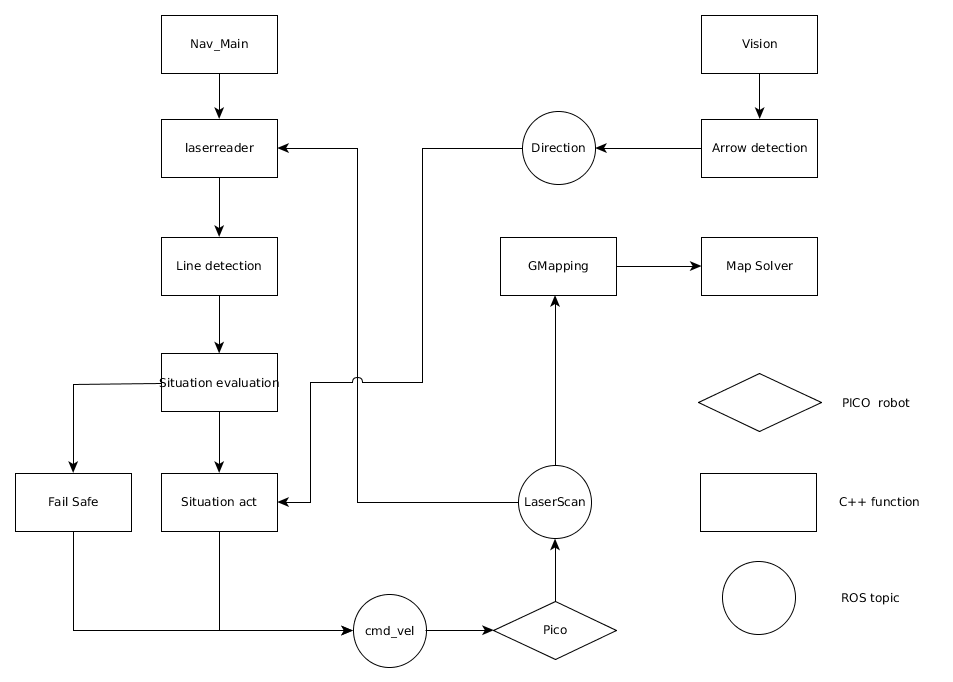

Unique Selling Point
- Home made line recognition and situation evaluator.
- Very robust Arrow Recognition
- Map generation and solving
- Modular set up of the code: very easy to add and/or remove functions
- Lightweight functions (especially line detection), leaving computational power for extra's
- Only used nodes when timing was not critical, increasing robustness
Final result
At the final test, Pico did not find the exit from the maze.
What went right
During the competition, Pico performed very well, driving the greatest distance without hitting any obstacle of any group. Other things that where succesful include:
- Lines were succesfully recognized and situations were (mostly) evaluated correctly
- A dead-end was recognized without actually going into it.
- The alignment in the corridors went perfectly.
- The arrow was recognized correctly and the appropriate action was taken.
Al this was observed through the states that were produced on the screen while Pico was going through the maze.
What went wrong (and why?)
- Map generation.
For the final test, all the files from the svn were moved to a local destination. Because we expected that the code would be run from the svn, as was the case in all our experiments, the "source" files did not contain the proper path. As of such, while a map was generated, the result could not be saved and hence we can not produce a result. However, since the code did work in all our simulations, experiments and with our bagfile, we assume that this was due to a copy fault. After the competition, we learned that there is a way to safeguard against this type of problem.
- Crossings
The first crossing went as expected, Pico tried to take the first right corner, but noted it was a dead end end turned 180 degrees to continue his journey (recognizing the other dead-end on his right side). However, in the second crossing, due to unkown reasons, Pico thought he was in a dead end and turned back again. Pico then drove on and recognized a dead end, which set him back on the proper route again. This time however; he did evaluate the situation correctly and turned right (as he should) at the appropriate time. We assume this loop occurred because a line was missed or not recognized in time. Since this behaviour was not observed in the simulation, it would be worthwhile to recreate this situation and test it in further experiments.
- Alignment in the T-junction with arrow
In the first T-junction (the first one with an arrow), the arrow was properly recognized and Pico turned to the correct direction. However, when Pico finished his turning, he was still inside the T-junction. His next observation was that he was in a corner, although a very wide one. He turned inward to align itself properly with the closest wall to the right and the wall to the left (in the crossing). As of susch, Pico to far inside and faced a wall. Since the direct vicinity of a wall was coded as a hard constraint, he drove back and tried to allign itself again. However, because his new position was now in the previous corridor, Pico then proceeded back into the maze. By then, the time was already running out (since 4 out of the 7 minutes were spent on copying the files). While it might have worked with a restart (Pico did finish the maze in the simulation), it did not come to that.
The last two situations could have been prevented with more time for testing and a bit of tuning of some parameters (especially the sleeptime of 0.05 seconds, increasing it could drastically alter the behaviour).
Evaluation
Because of the late and abrupt change in strategy, many functions where made and simulated but never were used on Pico; and the ones that where used were insufficiently tested. This might have been avoided with better communication, a recurring theme in group work. Another problem was that the amount of work was distributed rather unevenly over the time, which suggests that the planning was perhaps too vague and we should have been more rigid in setting our goals.
Recommendations
To improve the current code, most can be gained by making an (even more) intelligent situation evaluator, one that does not necessarily need to to know if a certain combination of lines and corners is a corner or a T-junction, but interprets the situation more humanlike and therefore, hopefully, more flexible. This proved too difficult to conceptualize in the last week, but it is a very interesting topic that might be further investigated.
Another improvement would be to include some sort of memory in the situation evaluator so it doesn't need to deduce from the current information that it is trying to complete a corner, but can simply rely on the memorized value. This would add value to the current program, and it would not be hard to implement.
Some of the search algorithms, such as in the corridor code where the wall on the right and on the left are searched for or the aligning, second part of the corner, could be made more robust by adding some extra checks whether or not the line found is the line that was searched for.
While our strategy was to evaluate each situation through the use of line recognition and pre-programmed situations, it would be better if all this could be avoided. For that, an entirely different concept is required which would work in a very different way. An optimal solution would allow Pico to drive trough any maze without any constrains on the situations he could encounter (thereby also allowing for curved walls, obstacles in the middle of the path, etc.) and would be (almost) independent of tuning. There are two such concepts that posses these properties: (1) The map generation with Dijkstra's Algorithm for path finding and (2) The Repulsive Force Field. Off course, both have their merits and disadvantages, and there exists no perfect method, but these are the concepts we would definitely try next.
A word of thanks
Finally, we would like to thank our tutor Yanick Douven for his help and guidance during the project. We learned a lot about designing software from him as well as all the problems and situations one has to think of if one wants the code to become even slightly robust.
