Mobile Robot Control 2021 Group 5: Difference between revisions
| (50 intermediate revisions by the same user not shown) | |||
| Line 27: | Line 27: | ||
=== Aligning to the walls === | === Aligning to the walls === | ||
As PICO has driven to a wall, it has to align itself to the wall. To do so, laser range finder data is used. The laser range finder should return the same distance at coefficients 0 and 220 for PICO to be alligned to the wall. In Figure | As PICO has driven to a wall, it has to align itself to the wall. To do so, laser range finder data is used. The laser range finder should return the same distance at coefficients 0 and 220 for PICO to be alligned to the wall. In Figure 2 it can be seen how the laser range finder coefficients are defined. As previously mentioned, PICO has driven to a nearby wall. Afterwards, it starts rotating quickly until the laser range finder data of coefficients 0 and 220 ratio is less than 0.2. Then it starts rotating slowly, until the laser range finder data of coefficients 0 and 220 ratio is less than 0.04. If this is the case, it is assumed PICO is alligned to the wall. | ||
[[File:Pico_schematic.png|none|450px|thumb|left|Figure | [[File:Pico_schematic.png|none|450px|thumb|left|Figure 2: Illustration of the laser range finder coefficients. ]] | ||
=== Driving along the wall === | === Driving along the wall === | ||
| Line 39: | Line 39: | ||
==== Centering in the Halway ==== | ==== Centering in the Halway ==== | ||
For the escape room challenge the decision is made to make the PICO center in the exit hallway. The idea is that this maximizes the distance to the walls and thus minimizes the chances of a collision. In applications where the robot may need to navigate a corridor where other dynamic objects are present, such as humans, it may be desirable to make the PICO drive on one side of the hallway. However, this is not the case for this challenge and thus a more robust solution is better. | For the escape room challenge the decision is made to make the PICO center in the exit hallway. The idea is that this maximizes the distance to the walls and thus minimizes the chances of a collision. In applications where the robot may need to navigate a corridor where other dynamic objects are present, such as humans, it may be desirable to make the PICO drive on one side of the hallway. However, this is not the case for this challenge and thus a more robust solution is better. | ||
Centering the PICO in the hallway is accomplished by measuring the distance to the walls at a pre-determined angle to the left and right from the normal direction of the PICO. On each side of the normal 20 datapoints are measured in a band around the set measurement angle α, as shown in the Figure | Centering the PICO in the hallway is accomplished by measuring the distance to the walls at a pre-determined angle to the left and right from the normal direction of the PICO. On each side of the normal 20 datapoints are measured in a band around the set measurement angle α, as shown in the Figure 3. The average of the 20 measured distances is then calculated to mitigate the affect of noise on the measurement. The distance to the left and right are then compared to each other and as long as they are within a certain range the PICO is centered. If they are not within the range the PICO moves either to the right or to the left to compensate. While the PICO is moving left or right it also continues to drive forward, in order to move as fast as possible. | ||
[[File:Pico_Halway_centering.png|none|450px|thumb|left|Figure | [[File:Pico_Halway_centering.png|none|450px|thumb|left|Figure 3: Illustration of the laser range finder coefficients. ]] | ||
== Results Escape Room Challenge == | == Results Escape Room Challenge == | ||
| Line 52: | Line 52: | ||
= Hospital challenge = | = Hospital challenge = | ||
== Strategy == | == Strategy == | ||
[[File:state_machine.png|none|700px|thumb|left|Figure | [[File:state_machine.png|none|700px|thumb|left|Figure 4: a graphical representation of the strategy at the hospital challenge]] | ||
The overall strategy can be seen in Figure | The overall strategy can be seen in Figure 4. However, the localization procedure and path planning itself need to be investigated so the best option in the hospital challenge will be used. | ||
== State Machine == | == State Machine == | ||
State Machine: | |||
An overview of the state machine used for the control of the robot can be seen in the figure 5. In this figure a distinction is made between the parts that are handled by ROS and the parts that are handled by custom C++ code. | |||
The PICO starts in the idle position where it goes to the initializing state when the start commando and the cabinet order is given. This information is processed and fed to the task manager. Furthermore, the initialization state features some pre-programed sequence to help the localization algorithm find the location and orientation of the PICO. The task manager keeps track of which cabinets have been visited and instructs the PICO to visit the next cabinet until the final cabinet is reached after which the program halts. These states are custom made in C++ and used to interface with the elements from ROS. | |||
The localizing state uses the AMCL algorithm to identify the location and orientation of the PICO. This information is then used for the path planning which happens in the planning state. The PICO is then actuated in the execution state, which follows the planned path. After a small portion of the path is executed the localization is performed again and the loop starts again. This loops makes it possible to identify and avoid unexpected and dynamic obstacles. | |||
When the executing state reaches the end of the planned path, the Finishing Task state is called. This state makes the PICO speak and saves a snapshot of the laser data. The task manager is then updated that the current task is finished and the next task will be called and executed. | |||
<gallery widths=600px heights=250px> | |||
File:state_machine.jpeg|Figure 5: State machine for the hospital challenge | |||
</gallery> | |||
== Localization procedure == | == Localization procedure == | ||
==== AMCL algorithm [4] ==== | ==== AMCL algorithm [4] ==== | ||
[[File:augumented_MCL.png|right|500px|thumb|left|Figure | [[File:augumented_MCL.png|right|500px|thumb|left|Figure 6: Pseudocode of the Adaptive Monte Carlo Localization ]] | ||
===== AMCL description ===== | ===== AMCL description ===== | ||
| Line 81: | Line 93: | ||
A pseudocode of the Adaptive Monte Carlo Localization is given in figure 8. It is a variant of the MCL algorithm that adds random particles. The first part is identical to the algorithm in MCL, where new poses are sampled from old particles using the motion model '''line 5''' and their importance weight is set in accordance to the measurment model '''line 6'''. However, '''Agumented_MCL''' calculates the emperical measurement likelihood in '''line 8''' and maintains short-term and long-term averages of this likelihood in '''line 10 and 11'''. During the resampling process a random sample is added with probability given in '''line 13'''. The probabilitiy of adding a random sample takes into consideration of the divergence between the short- and the long-term average of the measurment likelihood. If the short-term is better or equal to the long-term one, random smaples are added in proportion to the quotient of these values. In this way, a sudden decay in measuremnt likelihood induces an increased number of random samples. THe exponential smoothing counteracts the danger of mistaking sensor noise for a poor localization result. | A pseudocode of the Adaptive Monte Carlo Localization is given in figure 8. It is a variant of the MCL algorithm that adds random particles. The first part is identical to the algorithm in MCL, where new poses are sampled from old particles using the motion model '''line 5''' and their importance weight is set in accordance to the measurment model '''line 6'''. However, '''Agumented_MCL''' calculates the emperical measurement likelihood in '''line 8''' and maintains short-term and long-term averages of this likelihood in '''line 10 and 11'''. During the resampling process a random sample is added with probability given in '''line 13'''. The probabilitiy of adding a random sample takes into consideration of the divergence between the short- and the long-term average of the measurment likelihood. If the short-term is better or equal to the long-term one, random smaples are added in proportion to the quotient of these values. In this way, a sudden decay in measuremnt likelihood induces an increased number of random samples. THe exponential smoothing counteracts the danger of mistaking sensor noise for a poor localization result. | ||
== | ===== AMCL implementation ===== | ||
As for the implementation of the AMCL algorithm the AMCL package of ROS is used. The full description of the package with all its paramaters can be found in [7], as here only the tuned parameters and used methods are described. An important feature of the AMCL package of ROS is that a rough prediction of the position and forward direction of PICO needs to be given as an initial input. The location of PICO is known with an uncertainty of 1-by-1 meters. However, due to the fact that the forward direction of PICO is not known an initialization procedure needs to be written. More information on that can be found in the paragraph Initialization procedure. For now we consider that the intialization procedure works as expected and that the AMCL algorithm has produced an initial estimation on where PICO is located. Parameters that need to be tuned are listed below. Also a description is given on what effect this parameter has on the algorithm: | |||
- '''min_particles'''(100->500): This parameter determines how many particles should be used at least. Setting this too low and the algorithm will not be able to get a decent position estimation. Setting this too high and the algorithm will keep the amount of particles higher than necessary, which leads to longer computation time. We set this to 500 particles as it gave the most stable results when the AMCL procedure has a decent estimation of the location of PICO on the map.. | |||
- '''max_particles'''(5000->9000): This paramter determines the maximum allowed number of particles. Setting this too high and the computation time will exceed the update frequency leading to lag. Setting this too low and the algorithm will not be able to get a decent postion estimation when needed. We set this at 9000 particles as the number of particles decreases drasticly when the AMCL has localized PICO. This means that the amount of particles on average is much lower, but the algorithm localizes itself very fast when necessary. After each parameter name the original and tuned value (original -> tuned) are given to give an idea on what and by how much the parameter has changed. | |||
- '''laser_max_range'''(-1.0->10): This parameter determines the maximum range scan to be considerd. This parameter is set to 10.0m as this is the maximum range of the LIDAR. | |||
- '''laser_max_beams'''(30->250): This parameter determines how many evenly-spaced beams in ech scan are used when the filter is updated. As the range of PICO is quite large (220°) the value for this parameter was also increased to be 250, which means that at every 0.88° of range an object or feature can be used in the algorithm. When considering objects at the maximum length (10m), then only objects or features larger than 0.15m are considered certainly. | |||
- '''update_min_a''' (π/6.0->0.2): This parameter determines how much rotational movement needs to happen before the filter is updated. By decreasing this value the update frequency increases and aids the localization of faster moving dynamical objects. | |||
''' | Other parameters which are used for fine tuning and the prevention of lagging are: '''laser_z_hit''' (0.95->0.85), '''laser_z_short''' (0.1->1.0), '''laser_z_rand''' (0.05->0.15), '''laser_likelihood_max_dist''' (2.0m->10.0m) as the maximum LIDAR range is 10m, '''resample_interval''' (2->1) | ||
===== Initizalization procedure ===== | |||
== Path planning == | |||
Within this section, different path planning methods are investigated to see which method should be used in the hospital challenge. | |||
=== Global Path Planning === | |||
---- | |||
' | ==== Dijkstra's algorithm ==== | ||
[[File:Dijskra_algorithm.png|right|600px|thumb|left|Figure 8: Dijkstra's algorithm for finding the shortest path]] | |||
The Dijkstra's algorithm is an algorithm for finding the shortest paths between nodes in a graph. There are many variants of this algorithm, but the more common variant uses a fixed single "start" or "source" node and finds the shortest path to the "end" node producing a shortest path three. It systematically considers different node branches untill the algorithm knows for certain that it has found the shortest path. Dijkstra's algorithm uses the following function: | The Dijkstra's algorithm is an algorithm for finding the shortest paths between nodes in a graph. There are many variants of this algorithm, but the more common variant uses a fixed single "start" or "source" node and finds the shortest path to the "end" node producing a shortest path three. It systematically considers different node branches untill the algorithm knows for certain that it has found the shortest path. Dijkstra's algorithm uses the following function: | ||
''f(n) = g(n)'' | ''f(n) = g(n)'' | ||
where ''f'' is the total cost of the path, ''g'' is the cost to go from one node to another and ''n'' is the nodes. An example of how the Dijkstra alogorithm works is given in | where ''f'' is the total cost of the path, ''g'' is the cost to go from one node to another and ''n'' is the nodes. An example of how the Dijkstra alogorithm works is given in figure 8. First the algorithm looks at the costs of the path between the starting node S and node a and c. It determines that the cost to go from S-a is smaller than going from S-c, so it intially considers only S-a. The next steps are comparing path 1 to path 2, so the algorithm compares the cost of S-a-b with S-c. It knows that S-c has a smaller cost than S-a-b, so it considers this path. Next it does this until it eventually reaches the goal node G. In this example it considers all nodes, but when for example path 2 was much longer than path 1, then it would have discarded that path if path 1 reached the goal and had a lower cost than where path 2 has stranded. A downside of Dijkstra's algorithm is that it needs to consider a loth of nodes which are not in the direction of the goal. But this does make the algorithm complete and always produces the shortest path if there is one. The algorithm also uses a priority tree, which means that it firstly considers the path branch with the least cost. This can help in instances where one path branch is definitely faster/ less cost expensive than the other. An extension of this algorithm which is more efficient is described in the chapter below. | ||
==== A* search algorithm ==== | ==== A* search algorithm ==== | ||
| Line 133: | Line 138: | ||
<gallery widths=500px heights=250px> | <gallery widths=500px heights=250px> | ||
File:dijkstragif.gif|Figure | File:dijkstragif.gif|Figure 9: Dijkstra's algorithm for finding the shortest path [8] | ||
File:astartgif.gif|Figure | File:astartgif.gif|Figure 10: The A* algorithm for finding the shortest path [9] | ||
</gallery> | </gallery> | ||
==== | ==== A* search algorithm vs other algorithms ==== | ||
The decision for using the A* algorithm was made based on a comparison of different global path planning algorithms. There are a lot of different global planning algorithms available , but the most popular ones are compared with eachother. When comparing the A* algorithm with other algorithms such as the artificial potential field algorithm, visibility graph and Voronoi diagram different pros and cons become visible. | |||
The | |||
''' | The '''artifical potential field algorithm''' acts similarly as a charged particle where the robot is attracted to the target and repelled by obstacles as one can see in figure 7. The control input uses the attraction and repulsion factor to calculate the control input and the inputs are the weighted sum of both. These weights can be adapted to the specific needs of the path planning case. This algorithm has an advantage that parallel computing can be applied. This makes the compuational time much shorter and thus gives a faster solution. It is however difficult to implement parallel computing when no knowledge on how to implement this is known in advance. However, it is not optimal as it can produce local mimima which can trap PICO on a location on the map. There are methods available to prevent this, but it is a feature that needs to be cared of. This with an addition to the restricted available time has lead to decide that this algorithm will be discarded. | ||
The '''visibility graph''' method creates a path by connecting all points on the convex hull of the polygonal obstacles to each other, the agent and the goal. Then the shortest path is calculated which is the generated path. To accommodate for the width of the PICO, the PCIO can be modeled as a disk and the edges of the obstacles should be the offset by the radius of the disk. An example of the visibility graph is given in figure 8. This algorithm guarentees to find the shortest path, but it takes a lot of computing power as the graph needs to be recalculated when new objectes are discoverd. This also happens with the A* algorithm, but this algorithm handles dynamic obstacles better, so it was decided to use the A* algorithm and not the visibility graph. | |||
''' | The '''Voronoi diagram''' creates lines that are equidistant from all neighboring obstacles. These lines and their connections create the graph of all possible routes through the space. It can only give lines with pre-created points on the map which has a disadvantage when a lot of unknown obstacles are on the map as this would mean that a lot of arbitrarly chosen points need to be added. An example of the Voronoi diagram can be found in figure 9. It also has to include an algorithm like Dijkstra's or A* search algorithm to actually work. It is however faster than using only A* or Dijkstra as the shortest path search algorithms do not need to look to many points, but this also means that not always the shortest path is found. This algorithm will only be implemented in case the PICO does not have the required compuational power to use the A* algorithm, but in the meantime only the A* search algorithm is used. | ||
<gallery widths=300px heights=250px> | |||
File:potential.png|Figure 7: Representation on how the robot is attracted by the target and repelled by objects [1] | |||
File:visibility_graph.png|Figure 8: Example of a visibility graph [1] | |||
File:voronoi_diagram.png|Figure 9: example of a voronoi path planning graph. [2] | |||
</gallery> | |||
==== A* search algorithm implementation ==== | |||
==== | |||
=== Local Path Planning === | === Local Path Planning === | ||
| Line 234: | Line 222: | ||
[6] = https://www.sciencedirect.com/science/article/pii/S0921889016300495 | [6] = https://www.sciencedirect.com/science/article/pii/S0921889016300495 | ||
[7] = http://wiki.ros.org/amcl | |||
[8] = https://en.wikipedia.org/wiki/Dijkstra%27s_algorithm | |||
[9] = https://en.wikipedia.org/wiki/A*_search_algorithm | |||
Latest revision as of 08:53, 11 June 2021
Team members
Jaap van der Stoel - 0967407
Roel van Hoof - 1247441
Remco Kuijpers - 1617931 - r.kuijpers1@student.tue.nl - 0611135100
Timo de Groot - 1629352 - t.d.groot2@student.tue.nl
Roy Schepers - 0996153 - r.j.m.schepers@student.tue.nl - 0631329826
Arjan Klinkenberg - 1236143 - a.m.klinkenberg@student.tue.nl
Design document
- The Design Document: File:Design Document Group 5.pdf
Escape Room Challenge
Strategy
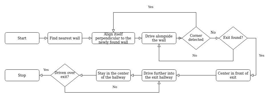
At The start of the escape room challange, the PICO searches for the closest wall. It then drives to this wall and allignes itself sideways to the wall. The PICO then drives straight ahead until either another wall, or the exit, is detected. In the first case the PICO rotates to align itself with the new wall and drives forwards again. In the second case the PICO rotates to align with the exit and then drives through the corridor of the finish line. A graphical representation of the strategy can be seen in Figure 1.
Implementation
Starting and finding nearest wall
At the start of the run the PICO will turn around 360 degrees to look for the wall which is closest to the PICO. When it has identified this direction it will turn to this direction and drive straight to this wall until it is 0.4m apart from the wall.
Aligning to the walls
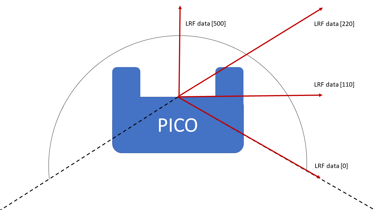
As PICO has driven to a wall, it has to align itself to the wall. To do so, laser range finder data is used. The laser range finder should return the same distance at coefficients 0 and 220 for PICO to be alligned to the wall. In Figure 2 it can be seen how the laser range finder coefficients are defined. As previously mentioned, PICO has driven to a nearby wall. Afterwards, it starts rotating quickly until the laser range finder data of coefficients 0 and 220 ratio is less than 0.2. Then it starts rotating slowly, until the laser range finder data of coefficients 0 and 220 ratio is less than 0.04. If this is the case, it is assumed PICO is alligned to the wall.
Driving along the wall
Now that PICO has aligned itself to the wall, it is going to drive alongside the wall. By doing so, multiple things can be sensed by the laser range finder. First off, if LRF data [500] senses a wall nearby, PICO stops, turns approximately 90 degrees, aligns itself to the wall, and starts to drive forward again. Secondly, if the ratio between LRF data [0] and [220] becomes too large, it is probable that a gap in the wall PICO is following is found. As a gap is found, PICO stops and is going to execute its exit procedure.
Exiting The Room
When PICO has identified an opening in to a wall it will start the exiting procedure. This will be done by turning around 90 degrees in the direction so that it faces the opening. It then drives sideways up to the point that it is in the middle of the exit corridor. PICO needs to drive forward and checks if it is not going too close to the wall.
Centering in the Halway
For the escape room challenge the decision is made to make the PICO center in the exit hallway. The idea is that this maximizes the distance to the walls and thus minimizes the chances of a collision. In applications where the robot may need to navigate a corridor where other dynamic objects are present, such as humans, it may be desirable to make the PICO drive on one side of the hallway. However, this is not the case for this challenge and thus a more robust solution is better. Centering the PICO in the hallway is accomplished by measuring the distance to the walls at a pre-determined angle to the left and right from the normal direction of the PICO. On each side of the normal 20 datapoints are measured in a band around the set measurement angle α, as shown in the Figure 3. The average of the 20 measured distances is then calculated to mitigate the affect of noise on the measurement. The distance to the left and right are then compared to each other and as long as they are within a certain range the PICO is centered. If they are not within the range the PICO moves either to the right or to the left to compensate. While the PICO is moving left or right it also continues to drive forward, in order to move as fast as possible.

Results Escape Room Challenge
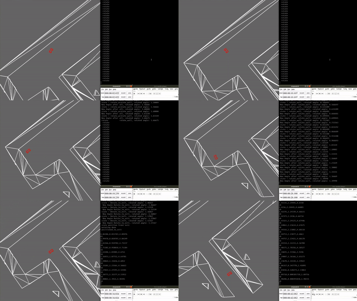
The escape room challenge is successfully complete and the PICO has escaped within 42 seconds, as can be seen in the video bellow.
Improvements
A few improvements can be considered and may aid in designing better software for the hospital challenge. One possible improvement is to decide, when aligning to the wall, what direction to turn would be the fastest. [add more improvements]
Hospital challenge
Strategy

The overall strategy can be seen in Figure 4. However, the localization procedure and path planning itself need to be investigated so the best option in the hospital challenge will be used.
State Machine
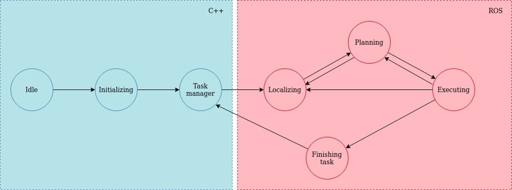
State Machine: An overview of the state machine used for the control of the robot can be seen in the figure 5. In this figure a distinction is made between the parts that are handled by ROS and the parts that are handled by custom C++ code.
The PICO starts in the idle position where it goes to the initializing state when the start commando and the cabinet order is given. This information is processed and fed to the task manager. Furthermore, the initialization state features some pre-programed sequence to help the localization algorithm find the location and orientation of the PICO. The task manager keeps track of which cabinets have been visited and instructs the PICO to visit the next cabinet until the final cabinet is reached after which the program halts. These states are custom made in C++ and used to interface with the elements from ROS.
The localizing state uses the AMCL algorithm to identify the location and orientation of the PICO. This information is then used for the path planning which happens in the planning state. The PICO is then actuated in the execution state, which follows the planned path. After a small portion of the path is executed the localization is performed again and the loop starts again. This loops makes it possible to identify and avoid unexpected and dynamic obstacles.
When the executing state reaches the end of the planned path, the Finishing Task state is called. This state makes the PICO speak and saves a snapshot of the laser data. The task manager is then updated that the current task is finished and the next task will be called and executed.
-
Figure 5: State machine for the hospital challenge
Localization procedure
AMCL algorithm [4]

AMCL description
The AMCL algorithm is an abbrivation of Adaptive Monte Carlo Localization, which is an extended version of Monte Carlo Localization (MCL). To understand the AMCL an explanation of MCL needs to be given first. MCL is a probabilistic localization system for a robot moving in 2D. It implements the Monte Carlo localization approach, which uses a particle filter to track the pose of a robot against a known map. The algorithm uses a particle filter to estimate its position throughout a known map. The initial global uncertainty is achieve through a set of pose particles drawn at random and uniformly over the entire pose space. When the robot sense a feature it gives a weight to the particle at that location. From the map data the algorithm assigns non-uniform importance weights to the likelihood of other features. Further motion leads to another resampling step where a new particle set is generated. Ultimately the location of features such as walls, corners, objects etc. will be estimated with a high accuracy and will eventually almost match the given map.
The size of the particle set M will determine the accuracy of the approximation. Increasing the size will lead to a higher accuracy, but this size is limited to the computational resources. A common strategy for setting M is to keep sampling particle until the next pair of measurements is arrived.
MCL solves the global localization problem, but cannot recover from robot kidnapping of global localization failures. In practice the MCL algorithm may accidentally discard all particles near a correct pose when being kidnapped. An Adaptive Monte Carlo Localization (AMCL) solves this problem. By adding random particles to the approximated particle sets the robot takes a probability into account that it may get kidnapped. This adds an additional level of robustness to the robot.
AMCL vs other algorithms
When comparing the AMCL algorithm to other popular algorithm such as an Extended Kalman Filter (EKF) or Multiple Hypothesis Tracking (MHT) some pros and cons become apparent. For example, the AMCL algorithm is much more robust than the EKF algorithm because it uses raw measurements to determine its pose instead of landmarks. This is especially important when the robot is kidnapped and no landmark is visible nearby. AMCL provides global localization while EKF and MHT can only provide local localization. AMCL is also much easier to implement compared to the MHT algorithm. A con of AMCL is that it is not as efficient in terms of memory and time compared to EKF and MHT. However it is still decided to use the AMCL algorithm due to its robustness, available global localization and because it solved the kidnap problem solving which cannot be solved easily with an EKF.
AMCL Pseudocode
A pseudocode of the Adaptive Monte Carlo Localization is given in figure 8. It is a variant of the MCL algorithm that adds random particles. The first part is identical to the algorithm in MCL, where new poses are sampled from old particles using the motion model line 5 and their importance weight is set in accordance to the measurment model line 6. However, Agumented_MCL calculates the emperical measurement likelihood in line 8 and maintains short-term and long-term averages of this likelihood in line 10 and 11. During the resampling process a random sample is added with probability given in line 13. The probabilitiy of adding a random sample takes into consideration of the divergence between the short- and the long-term average of the measurment likelihood. If the short-term is better or equal to the long-term one, random smaples are added in proportion to the quotient of these values. In this way, a sudden decay in measuremnt likelihood induces an increased number of random samples. THe exponential smoothing counteracts the danger of mistaking sensor noise for a poor localization result.
AMCL implementation
As for the implementation of the AMCL algorithm the AMCL package of ROS is used. The full description of the package with all its paramaters can be found in [7], as here only the tuned parameters and used methods are described. An important feature of the AMCL package of ROS is that a rough prediction of the position and forward direction of PICO needs to be given as an initial input. The location of PICO is known with an uncertainty of 1-by-1 meters. However, due to the fact that the forward direction of PICO is not known an initialization procedure needs to be written. More information on that can be found in the paragraph Initialization procedure. For now we consider that the intialization procedure works as expected and that the AMCL algorithm has produced an initial estimation on where PICO is located. Parameters that need to be tuned are listed below. Also a description is given on what effect this parameter has on the algorithm:
- min_particles(100->500): This parameter determines how many particles should be used at least. Setting this too low and the algorithm will not be able to get a decent position estimation. Setting this too high and the algorithm will keep the amount of particles higher than necessary, which leads to longer computation time. We set this to 500 particles as it gave the most stable results when the AMCL procedure has a decent estimation of the location of PICO on the map..
- max_particles(5000->9000): This paramter determines the maximum allowed number of particles. Setting this too high and the computation time will exceed the update frequency leading to lag. Setting this too low and the algorithm will not be able to get a decent postion estimation when needed. We set this at 9000 particles as the number of particles decreases drasticly when the AMCL has localized PICO. This means that the amount of particles on average is much lower, but the algorithm localizes itself very fast when necessary. After each parameter name the original and tuned value (original -> tuned) are given to give an idea on what and by how much the parameter has changed.
- laser_max_range(-1.0->10): This parameter determines the maximum range scan to be considerd. This parameter is set to 10.0m as this is the maximum range of the LIDAR.
- laser_max_beams(30->250): This parameter determines how many evenly-spaced beams in ech scan are used when the filter is updated. As the range of PICO is quite large (220°) the value for this parameter was also increased to be 250, which means that at every 0.88° of range an object or feature can be used in the algorithm. When considering objects at the maximum length (10m), then only objects or features larger than 0.15m are considered certainly.
- update_min_a (π/6.0->0.2): This parameter determines how much rotational movement needs to happen before the filter is updated. By decreasing this value the update frequency increases and aids the localization of faster moving dynamical objects.
Other parameters which are used for fine tuning and the prevention of lagging are: laser_z_hit (0.95->0.85), laser_z_short (0.1->1.0), laser_z_rand (0.05->0.15), laser_likelihood_max_dist (2.0m->10.0m) as the maximum LIDAR range is 10m, resample_interval (2->1)
Initizalization procedure
Path planning
Within this section, different path planning methods are investigated to see which method should be used in the hospital challenge.
Global Path Planning
Dijkstra's algorithm
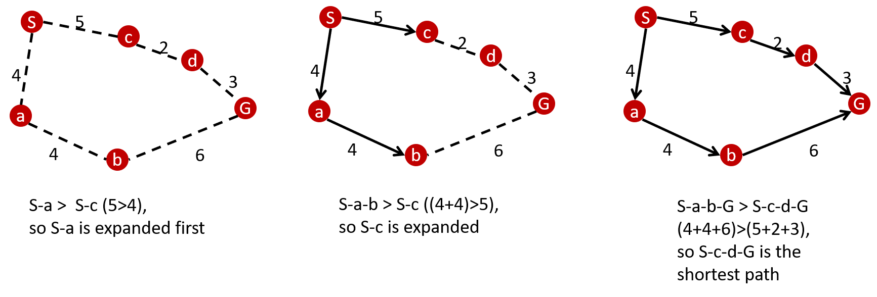
The Dijkstra's algorithm is an algorithm for finding the shortest paths between nodes in a graph. There are many variants of this algorithm, but the more common variant uses a fixed single "start" or "source" node and finds the shortest path to the "end" node producing a shortest path three. It systematically considers different node branches untill the algorithm knows for certain that it has found the shortest path. Dijkstra's algorithm uses the following function:
f(n) = g(n)
where f is the total cost of the path, g is the cost to go from one node to another and n is the nodes. An example of how the Dijkstra alogorithm works is given in figure 8. First the algorithm looks at the costs of the path between the starting node S and node a and c. It determines that the cost to go from S-a is smaller than going from S-c, so it intially considers only S-a. The next steps are comparing path 1 to path 2, so the algorithm compares the cost of S-a-b with S-c. It knows that S-c has a smaller cost than S-a-b, so it considers this path. Next it does this until it eventually reaches the goal node G. In this example it considers all nodes, but when for example path 2 was much longer than path 1, then it would have discarded that path if path 1 reached the goal and had a lower cost than where path 2 has stranded. A downside of Dijkstra's algorithm is that it needs to consider a loth of nodes which are not in the direction of the goal. But this does make the algorithm complete and always produces the shortest path if there is one. The algorithm also uses a priority tree, which means that it firstly considers the path branch with the least cost. This can help in instances where one path branch is definitely faster/ less cost expensive than the other. An extension of this algorithm which is more efficient is described in the chapter below.
A* search algorithm
The A* search algorithm can be interpeted as an "optimal" version of the Dijkstra's algorithm as it is an optimized version of the Dijkstra's algorithm in terms of efficiency. In this context, optimal does not mean that it reaches the optimal solution, but that it does so while exploring the minimum number of nodes. It differs from its precessor because it uses a heursitc function h(n) where n is the next node on the path. A heuristic technique is any approach to problem solving that does not immediatly guarantee the perfect solution, but is sufficient enough for reaching the short-term goal of approximation fast. This makes the algorithm less energy and computational consuming which is an important aspect for a mobile robot with limited battery duration and computational power. This is also visible in the animations below where the Dijkstra's algorithm and A* algorithm are compared to each other. A* selects a path which minimizes
f(n) = g(n) + h(n)
where n is the next node on the path, g(n) is the cost of the path from the start node to n and h(n) is the heuristic function that estimates the cost of the cheapest path from n to the goal. When h(n) is adimissable it never overstimates the optimal path to get to the goal from the current node. It will hence guarantee to return a least-cost path from start to goal.
-
Figure 9: Dijkstra's algorithm for finding the shortest path [8]
-
Figure 10: The A* algorithm for finding the shortest path [9]
A* search algorithm vs other algorithms
The decision for using the A* algorithm was made based on a comparison of different global path planning algorithms. There are a lot of different global planning algorithms available , but the most popular ones are compared with eachother. When comparing the A* algorithm with other algorithms such as the artificial potential field algorithm, visibility graph and Voronoi diagram different pros and cons become visible.
The artifical potential field algorithm acts similarly as a charged particle where the robot is attracted to the target and repelled by obstacles as one can see in figure 7. The control input uses the attraction and repulsion factor to calculate the control input and the inputs are the weighted sum of both. These weights can be adapted to the specific needs of the path planning case. This algorithm has an advantage that parallel computing can be applied. This makes the compuational time much shorter and thus gives a faster solution. It is however difficult to implement parallel computing when no knowledge on how to implement this is known in advance. However, it is not optimal as it can produce local mimima which can trap PICO on a location on the map. There are methods available to prevent this, but it is a feature that needs to be cared of. This with an addition to the restricted available time has lead to decide that this algorithm will be discarded.
The visibility graph method creates a path by connecting all points on the convex hull of the polygonal obstacles to each other, the agent and the goal. Then the shortest path is calculated which is the generated path. To accommodate for the width of the PICO, the PCIO can be modeled as a disk and the edges of the obstacles should be the offset by the radius of the disk. An example of the visibility graph is given in figure 8. This algorithm guarentees to find the shortest path, but it takes a lot of computing power as the graph needs to be recalculated when new objectes are discoverd. This also happens with the A* algorithm, but this algorithm handles dynamic obstacles better, so it was decided to use the A* algorithm and not the visibility graph.
The Voronoi diagram creates lines that are equidistant from all neighboring obstacles. These lines and their connections create the graph of all possible routes through the space. It can only give lines with pre-created points on the map which has a disadvantage when a lot of unknown obstacles are on the map as this would mean that a lot of arbitrarly chosen points need to be added. An example of the Voronoi diagram can be found in figure 9. It also has to include an algorithm like Dijkstra's or A* search algorithm to actually work. It is however faster than using only A* or Dijkstra as the shortest path search algorithms do not need to look to many points, but this also means that not always the shortest path is found. This algorithm will only be implemented in case the PICO does not have the required compuational power to use the A* algorithm, but in the meantime only the A* search algorithm is used.
-
Figure 7: Representation on how the robot is attracted by the target and repelled by objects [1]
-
Figure 8: Example of a visibility graph [1]
-
Figure 9: example of a voronoi path planning graph. [2]
A* search algorithm implementation
Local Path Planning
TEB local planner

All information below about the TEB algorithm is taken from [5, 6] and is reworded to fit the format of the wiki and project.
The TEB (Timed Elastic Bands) approach is a method for path planning for autonomous robots that minimizes the time while taking (kino-)dynamic constraints, such as maximum velocity and acceleration, into account. Using only the TEB approach will often lead to locally optimal solutions instead of the desired globally optimal solutions. This is due to the fact that the TEB approach smoothly transforms the planed path based on detected obstacles, but doesn’t consider alternative paths. To make sure the path finding algorithm finds the optimal path the TEB algorithm is extended. This extension enables the path planner to optimize a subset of admissible trajectories of distinctive topologies in parallel. Distinctive topologies in this context means, paths that belong to different homologous classes. A distinction is made between homotopic paths and homologous paths. Below follow the definitions.
Definition: Homotopic Paths
Two paths are homotopic if they have the same start and end points, and can be continuously deformed into each other without intersecting any obstacles. A homotopy class is then the set of all paths than are homotopic to each other.
Definition: Homologous Paths
Two paths τ1 and τ2 with the same start and end point, are homologous if and only if τ1⊔−τ2 forms the complete boundary of a 2D manifold embedded in C not containing and intersecting any obstacle. A homology class is then a set of all paths homologous to eachother.
Homology classes are easier to compute and therefore better suited for an online path planner for autonomous robots. This is the reason why Homology classes are used instead of homotopic classes for the path finding algorithm. The extended TEB algorithm then optimizes (w.r.t. time) multiple path in parallel all belonging to different homologous classes, and has the ability to switch to the current global optimal solution.
The extended TEB algorithm consists of two parts: first a part that finds alternative homology classes and secondly a part that optimizes the path in each homology class. Both parts are explained below.
Part 1: Identifying different homology classes
In order to find different homology classes, each acceptable path gets an associated H-signature. This is a number that is the same for each path within a certain homology class but is different for paths between different classes. The paths are discretized and therefore consist of line segments connecting two points zk and zk+1.
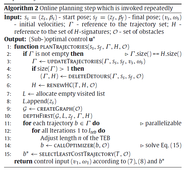
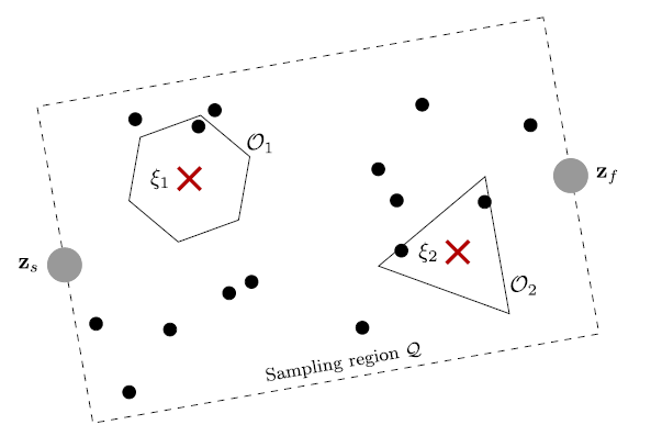
There are different ways to explore acceptable path and calculate the H-signatures. For example using a Voronoi diagram will give a complete exploration graph within al feasible paths. However using a Voronoi diagram is very expensive w.r.t. comuter calculations. Therefore a sample based system is used. This system creates a closed area between the start and end point and uniformly samples waypoints within this area. Waypoints that intersect with any obstacle region are removed and new waypoints are sampled until the set number of waypoints is reached. The placed waypoints are then connected to each other if this connection decreases the Euclidian distance to the goal and a connecting line segment does not intersect an obstacle. The H-signature for each constructed path from the start to the end point is calculated and the different homology classes are determined. The sampling of the waypoints is repeated with each step in order to discover new homology classes that were previously not jet detected. Figure 9 showhs the psudocode of the algorithm used to identify the different homolgy classes. Figure 10 shows an example region with sampled waypoints, where zs is the starting point and zf is the end point.
Part 2: optimizing the path within a homology class
To optimize the path in each homology class the TEB algorithm is used. The TEB algorithm is implemented as an approximate optimizer that uses user defined weights for the cost function. This is done to improve the computational efficiency of the algorithm. Figure 11 shows the implementation of the TEB algorithm in combination with algorithm 1 (line 10).
Clip 2 shows a demo of how the extended TEB algorithm works. The green lines are the optimized paths from each homology class. The path with the green arrows is the globally optimal path that has been found.
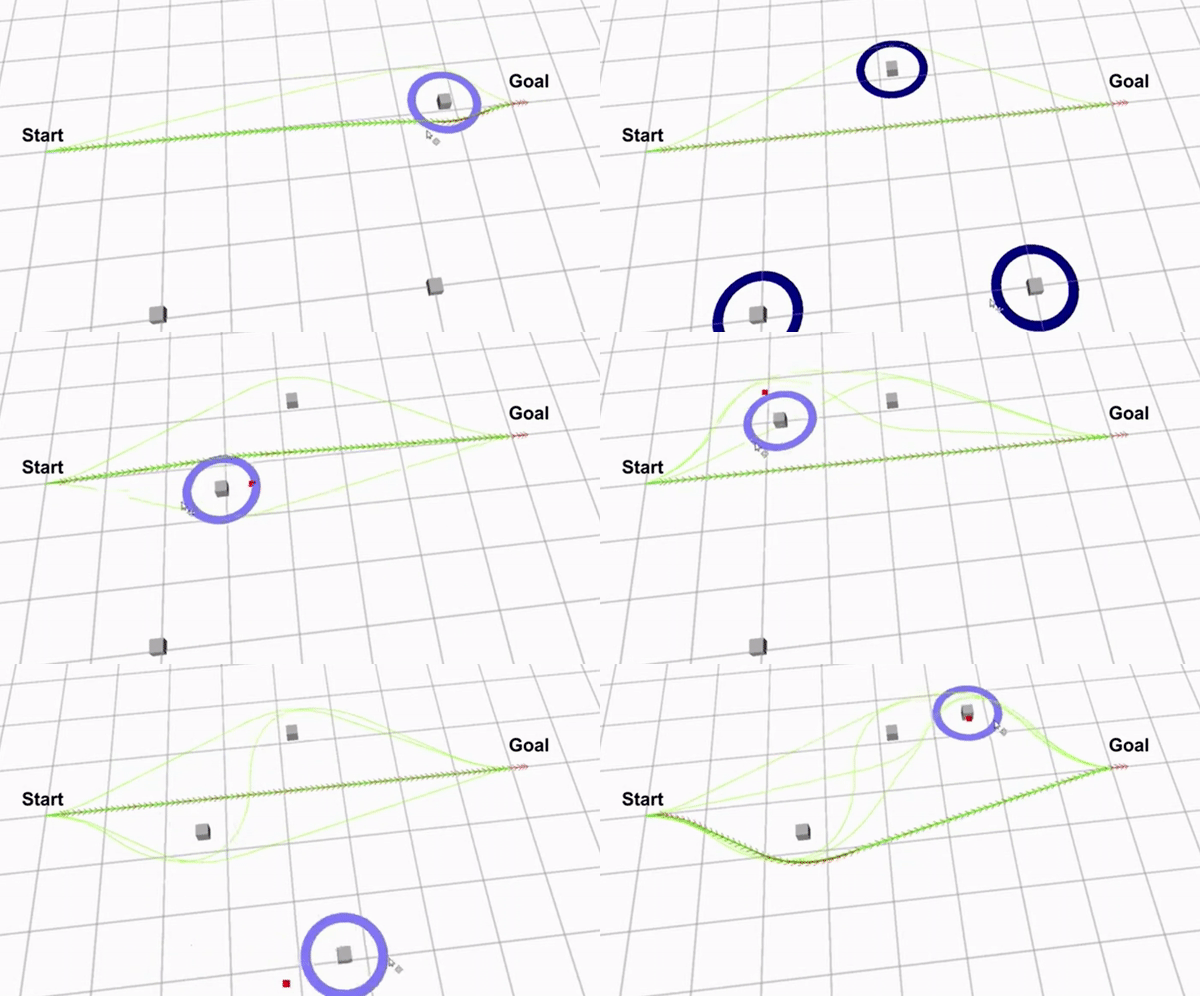
Although the extended TEB algorithm could be used as a global path planning algorithm, this would be a very expensive algorithm in terms of computer calculations. Therefore The extended TEB algorithm is used as a local path planner, to avoid unexpected obstacles. The extended TEB algorithm is a good choice for the hospital challenge since it can handle dynamic obstacles very well. Furthermore the goal of the hospital challenge is to complete the tasks as fast as possible, therefore a path planning algorithm that minimizes time is very useful. The final reason to use the extend TEB algorithm is that it is easy to implement using ROS and the “teb_local_planner” package.
References
[4]= Thrun, S. (2002). Probabilistic robotics. Communications of the ACM, 45(3), 52–57. https://doi.org/10.1145/504729.504754
[5] = http://wiki.ros.org/teb_local_planner
[6] = https://www.sciencedirect.com/science/article/pii/S0921889016300495
[7] = http://wiki.ros.org/amcl
![Figure 9: Dijkstra's algorithm for finding the shortest path [8]](/images/Dijkstragif.gif)
![Figure 10: The A* algorithm for finding the shortest path [9]](/images/Astartgif.gif)
![Figure 7: Representation on how the robot is attracted by the target and repelled by objects [1]](/images/Potential.png)
![Figure 8: Example of a visibility graph [1]](/images/Visibility_graph.png)
![Figure 9: example of a voronoi path planning graph. [2]](/images/Voronoi_diagram.png)