Mobile Robot Control 2021 Group 1: Difference between revisions
TUe\20172912 (talk | contribs) No edit summary |
TUe\20172912 (talk | contribs) No edit summary |
||
| (7 intermediate revisions by the same user not shown) | |||
| Line 136: | Line 136: | ||
[[File:Formula.JPG|300px|Point cloud formula]] | [[File:Formula.JPG|300px|Point cloud formula]] | ||
After computation of the point cloud, the algorithm introduced by Peter et al. (Figure 4) was used to translate this point cloud into a line segmentation. | After the computation of the point cloud, the algorithm introduced by Peter et al. (Figure 4) was used to translate this point cloud into a line segmentation. | ||
<h4>Finding the line segments</h4> | <h4>Finding the line segments</h4> | ||
The world model approach is based on research by Peter et al. (2017) was used. Peter et al. map 2D laser input to line segmentation based on a range of residuals. To use this approach, it was necessary to compute the point cloud from the 1000 laser beams retrieved from the LRF. Computation was done based on the following formula: | The world model approach is based on research by Peter et al. (2017) was used. Peter et al. map 2D laser input to line segmentation based on a range of residuals. To use this approach, it was necessary to compute the point cloud from the 1000 laser beams retrieved from the LRF. Computation was done based on the following formula: | ||
| Line 142: | Line 142: | ||
'''The Kalman Filter''' <br> | '''The Kalman Filter''' <br> | ||
The Kalman filter can be split into 4 parts: initialization, prediction, measurement, and update. As can be seen in the figure. | The Kalman filter can be split into 4 parts: initialization, prediction, measurement, and update. As can be seen in the figure. | ||
[[File:KalmanSchedule.png|800px|center| Figure | [[File:KalmanSchedule.png|800px|center| Figure: Schematic representation of the Kalman filter.]] | ||
'''Initialization''' <br> | '''Initialization''' <br> | ||
In the initialization step, the initial configuration and covariance of PICO are given to the Kalman filter. It is of high importance that the initial configuration and covariance is accurately estimated, since it is the foundation for the following steps. There will be an intial starting area given for the competition. Thus, the LiDAR data will be fitted for this area to find the intial configuration of PICO. <br> | |||
'''Prediction''' <br> | '''Prediction''' <br> | ||
In the prediction step, the data obtained from the previous iteration and the data from the odometry are used to predict the new data. The data is described in terms of a reference frame, which is frame O in the figure below. The data measured with the odometry is the configuration of frame 1 with respect to frame 0. This data can be transformed to the configuration of frame 1 with respect to frame O. <br> | |||
[[File:ReferenceFrame.png|300px|center| Figure: Reference Frame]] | |||
The predicted configuration is obtained by adding up the configuration of the previous iteration and the transformed odometry data. As can be seen in the equations: <br> | |||
[[File:OdomData1.PNG|300px|Odometry data equation 1]]<br> | |||
The predicted covariance is obtained with the previous covariance, the odometry covariance, the configuration change between the two iterations described in the reference frame O. The odometry covariance is retrieved by calculating the covariance of the movement forward, movement side-ways, and the turn. <br> | |||
[[File:OdomData2.PNG|400px|Odometry data equation 1]] <br> | |||
'''Measurement''' <br> | '''Measurement''' <br> | ||
In the measurement step, the data obtained from the LRF sensors are fitted on the map to determine the configuration and standard deviation. This is done by... <br> | |||
'''Update''' <br> | '''Update''' <br> | ||
In the update step, the data of both the predition step and the measurement step are weighted to determine the actual configuration. <br> | |||
<h4>Generating the world model</h4> | <h4>Generating the world model</h4> | ||
<h4>Initializing the static map</h4> | <h4>Initializing the static map</h4> | ||
Latest revision as of 16:47, 26 May 2021
Members
- Véronne Reinders (v.reinders@student.tue.nl) - 1706837
- Danique van Berlo (d.y.b.m.v.berlo@student.tue.nl) - 1242645
- Tim van de Ven (n.c.m.v.d.ven@student.tue.nl) - 0948317
- Daan Roordink (d.roordink@student.tue.nl) - 0863456
- Yu-Hsin Wu (y.h.wu@student.tue.nl) - 1623141
- Mike van Duijnhoven (m.p.j.v.duijnhoven@student.tue.nl) - 1510266
Planning
| Week | Deadlines | Done before weekly meeting 1 | Done before weekly meeting 2 |
|---|---|---|---|
| 1 (19/04-25/04) | |||
| 2 (26/04-02/05) | Read the wiki page carefully | First draft of the design document | |
| 3 (03/05-09/05) | 04/05 - Design Document | Adjust the design document and have all software working | Finalize the design document and first draft of strategy for the escape room |
| 4 (10/05-16/05) | 12/05 - Escape room competition | Finalize the strategy for the escape room | Work on two parts of the hospital strategy:
|
| 5 (17/05-23/05) | Work on parts of the hospital strategy:
|
Work on parts of the hospital strategy:
| |
| 6 (24/05-30/05) | Work on parts of the hospital strategy:
|
Work on parts of the hospital strategy:
| |
| 7 (31/05-06/05) | 02/06 - Presentation | Adjust the strategy for the final competition | Adjust the strategy for the final competition |
| 8 (07/06-13/05) | 09/06 - Final competition | Finalize the strategy for the final competition | Debrief the competition for recommendations for future work |
| 9 (14/06-20/05) | Adjust the wiki page where needed | Finalize the wiki page | |
| 10 (21/06-27/05) | 23/06 - Wiki page |
Design Document
The design document can be found here and contains our interpretation of the requirements, functions, components, specifications and interfaces for both the escape room and hospital challenge.
Escape room competition
Strategy
In the escape room competition, PICO will first simply drive forward until PICO finds a wall. When PICO is at a certain distance from the wall, it will start to turn until the wall is on its right side and parallel to its driving direction. Afterward, PICO will follow the wall and the following corners. This will go on until PICO passes the finish.
Software implementation

state: intialization named "init" PICO will continuously check if it is close to a wall.
- If PICO is close to a wall, the state will change to "followWall".
- Otherwise, PICO will drive forward.
state: follow the wall named "followWall" PICO will update its detected distance from the wall continuously. Meanwhile, updating PICO moves according to its distance from the wall
- If PICO his detected distance from the wall is too far, PICO will rotate towards the wall.
- If PICO his detected disctance from the wall is too close, PICO will rotate from teh wall.
- If PICO encounters a convex corner, the state will change to "driveInto".
- If PICO encounters a concave corner??, the state will change to "turn".
- Otherwise, PICO will drive forward.
state: turning 45 degrees named "turn" The angle with respect to the start of the turn is measured.
- If the angle is smaller than 45 degrees, PICO will rotate.
- Otherwise, the state will change to "followWall"
state: passing the convex corner "driveInto" The x, y distance and angle with respect to the start of the state is measured.
- If the measured total distance w.r.t. to the start of the state is smaller than 0.5m, PICO will drive forward.
- If the measured angle is smaller than 90 degrees, PICO will rotate.
- Otherwise, the state will change to "followWall"
Use cases
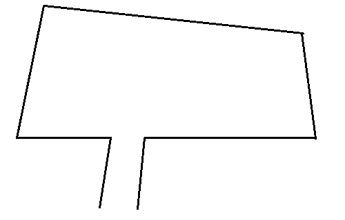
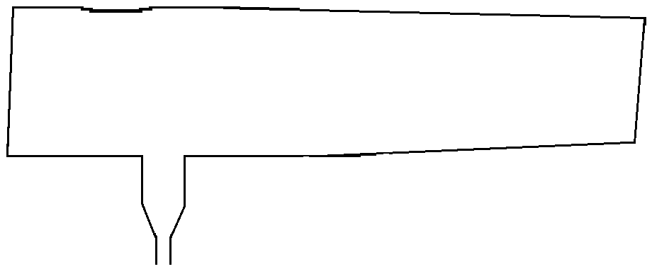
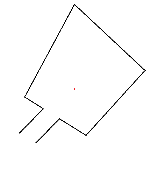
To make sure PICO will perform as expected during the competition, a couple of use cases are made to test its performance. The use cases are several different maps and different configurations within those maps. In these maps the environment specifications, such as crooked corners and walls but also a very small room or very large room, are incorporated as good as possible. The image name, the word thumb then the caption :
-
Figure 2a: Test map 1; where the difficulty is in the crooked walls and corridor.
-
Figure 2b: Test map 2; where the difficulty is in the bump in the wall.
-
Figure 2c: Test map 3; where the difficulty is that PICO drives straight into a corner.
Hospital competition
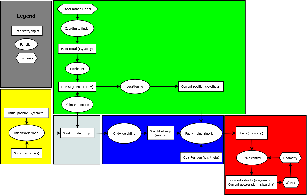
For the Hospital competition, the basic information flow diagram is shown in Figure 3. Starting from the input of the LRF data, the data is transformed using several functions. After obtaining the world model, the starting map can be initialized. Then, path planning can start. In order to do so, a weighted map has to be generated first. Then, by using the current position and goal positions, the (current) optimal path can be generated. This path can then be used by the drive controller to move the robot. By using a 20Hz iteration procedure, the optimal path can be updated according to new findings, such as closed doors or moving objects.
Obtaining the point cloud
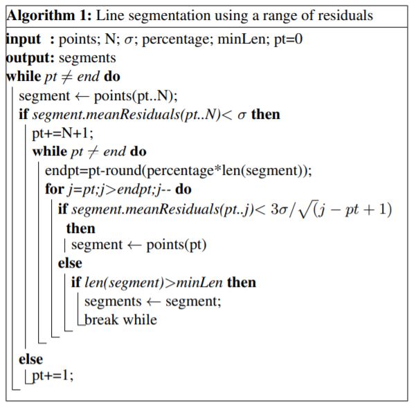
After the computation of the point cloud, the algorithm introduced by Peter et al. (Figure 4) was used to translate this point cloud into a line segmentation.
Finding the line segments
The world model approach is based on research by Peter et al. (2017) was used. Peter et al. map 2D laser input to line segmentation based on a range of residuals. To use this approach, it was necessary to compute the point cloud from the 1000 laser beams retrieved from the LRF. Computation was done based on the following formula:
Finding the current position
The Kalman Filter
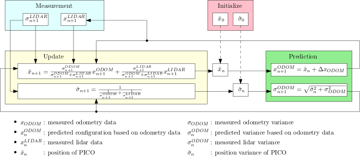
The Kalman filter can be split into 4 parts: initialization, prediction, measurement, and update. As can be seen in the figure.
Initialization
In the initialization step, the initial configuration and covariance of PICO are given to the Kalman filter. It is of high importance that the initial configuration and covariance is accurately estimated, since it is the foundation for the following steps. There will be an intial starting area given for the competition. Thus, the LiDAR data will be fitted for this area to find the intial configuration of PICO.
Prediction
In the prediction step, the data obtained from the previous iteration and the data from the odometry are used to predict the new data. The data is described in terms of a reference frame, which is frame O in the figure below. The data measured with the odometry is the configuration of frame 1 with respect to frame 0. This data can be transformed to the configuration of frame 1 with respect to frame O.
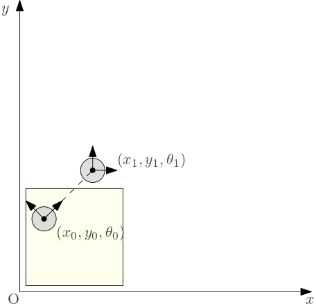
The predicted configuration is obtained by adding up the configuration of the previous iteration and the transformed odometry data. As can be seen in the equations:
The predicted covariance is obtained with the previous covariance, the odometry covariance, the configuration change between the two iterations described in the reference frame O. The odometry covariance is retrieved by calculating the covariance of the movement forward, movement side-ways, and the turn.

Measurement
In the measurement step, the data obtained from the LRF sensors are fitted on the map to determine the configuration and standard deviation. This is done by...
Update
In the update step, the data of both the predition step and the measurement step are weighted to determine the actual configuration.
Generating the world model
Initializing the static map
Formulating the weighted map
In order to formulate the weighted map, a gridmap had to be specified first. This was done by using the provided static map. By finding the given maximum and minimum coordinates, a good estimate of the size of the map can be formulated. Then, a grid based on these coordinates can be given. In example, when the provided JSON static map coordinates are (x,y) = (5,6) meters, and the minumum is (x,y) = (-1,-2) meters. Then the total grid size is (6,8) meters. Then, by dividing this with the wanted grid size (e.g. 0.1 meters), a grid can be obtained. This grid was formulated in a matrix, with size: (xmax-xmin/0.1,ymax-ymin/0.1), given 0.1x0.1 meter grid boxes.
With this grid matrix, weights can be imported and updated using LRF measurement data by using an
Path Planning
We are dealing with a motion planning problem where the goal is to compute a path between the starting point and the goal. We can solve a low-dimensional problem by overlaying a grid on the world model. Within this grid, we can identify which grid points are walls or are within a certain distance from the wall, with a minimum of PICO’s height (given that it has one, because of the holonomic drivetrain, PICO can maneuver sideways). All the other free space can be considered for finding the shortest path with A*. This grid is also known as a weighted map. A* uses a heuristic to guide itself, just like greedy best-first-search. A* examines the path that has the lowest f(n) = g(n) + h(n). Where g(n) is the exact cost (like for the Dijkstra’s algorithm) from starting point to any vertex n. h(n) is the heuristic estimated cost from that vertex n to the goal node. The heuristic can be calculated in different ways: Manhattan distance, diagonal distance, and Euclidean distance. Since PICO is allowed to/can move in every direction we will be using the Euclidean distance to calculate the heuristic for the hospital challenge. The edges of the graph will be the distance between two vertices. Because A* works in such a way that it makes a decision every step of the way, PICO can move forward with these decisions. This helps because closed doors or dynamic objects will be detected and can then be added to the weighted map and we can compute the next shortest path from there.
The drive control
Meeting Notes
26/04/2021
Get requirements from the Wiki and the slides. Components are in the slides as well.
30/04/2021
Include meeting notes on Wiki.
The Wiki will be the final report. So if you update it weekly with the progress and findings it will save us a lot of time in the end.
Final: complete description of the system, role division, etc.
General availability: Tuesday and Thursday
Action Points
- Find a weekly meeting moment - Tuesday 9.00 (tutor meeting from 10.00) & Friday 13.30
- Make a general planning: Danique
- Finish the design document - Everyone - Deadline Monday 22.00
04/05/2021
Action Points
- Finish the design document: Mike, Daan and Tim
- Review the design document and upload it on the wiki before 16.55: Daan
- Individually start on the programming and get familiar with the code before Friday: Everyone
- Select the best working code on Friday and split up the work from there on
07/05/2021
From now on meetings will be with an agenda and in between SSAs will be made. To find the specifics of the meeting read the notes on the drive.
Action Points
- Work on the dumb approach: Mike, Danique, Yu Hsin
- Work on the word model (approach): Daan, Tim, Veronne
- Upload a SSA template: Tim
- Make a git ignore: Daan
11/05/2021
Action Points
- Finish the wall-following approach: Mike, Danique, Yu Hsin
- Look into best approach for localization: Mike, Danique, Yu Hsin
- Work on the word model (approach): Daan, Tim, Veronne
14/05/2021
We did quite well in the escape room competition, by escaping in 44 seconds. However, some implementation of communication from PICO is missing such as SLAM or sound.
Action Points
- Determine a strategy: Tim
- Decide on a pathfinding method: Veronne
- Work on the visualization: Yu Hsin
- Work on extended Kalman filter for localization: Mike and Danique
- PICO detects line the line segments: Mike and Daan
18/05/2021
There are some uncertainties about the doors in the map and if A* can deal with all dynamic objects.
Action Points
- Work on the pathfinding method: Tim and Veronne
- Finish the visualization: Yu Hsin
- Work on the extended Kalman filter: Daan, Mike and Danique
21/05/2021
There are some uncertainties about the doors in the map and if A* can deal with all dynamic objects.
Action Points
- Work on the pathfinding method: Tim and Veronne
- Add obstacles to the visualization: Yu Hsin
- Work on the localization: Daan, Mike and Danique
25/05/2021
There are some uncertainties about the doors in the map and if A* can deal with all dynamic objects.
Action Points
- Work on the pathfinding method: Tim and Veronne
- Look into the path following method: Tim
- Work on the interaction with the cabinets: Yu Hsin
- Work on the Localization: Daan, Mike and Danique
- Make the presentation: Tim and Danique
