Mobile Robot Control 2021 Group 3: Difference between revisions
TUe\s163167 (talk | contribs) |
|||
| (4 intermediate revisions by 3 users not shown) | |||
| Line 100: | Line 100: | ||
<h5>2. Corridor and edge detection</h5> | <h5>2. Corridor and edge detection</h5> | ||
As previously mentioned, in the Escape Room Challenge, one is faced with one room with one corridor. It is therefore key to classify the angles between two line segments as either convex or concave. In case the angle is concave PICO recognizes this as a corner and if it is convex it is classified as an edge. The two points which are the most convex are assumed to be | As previously mentioned, in the Escape Room Challenge, one is faced with one room with one corridor. It is therefore key to classify the angles between two line segments as either convex or concave. In case the angle is concave PICO recognizes this as a corner and if it is convex it is classified as an edge. The two points which are the most convex are assumed to be the edges of the corridor. The target position is placed in the middle of these, i.e. it is assumed to be the entrance of the corridor. Worth noticing is that PICO keeps scanning while driving towards the previously set target, if it finds a more suitable corridor edge the target will be recalculated. | ||
== Results of the Escape Room Challenge == | == Results of the Escape Room Challenge == | ||
| Line 119: | Line 119: | ||
= Hospital Challenge = | = Hospital Challenge = | ||
==Path Planning== | ==Path Planning== | ||
For the robot to reach every cabinet in a specified order it needs to know how to get from one cabinet to the next. Here path planning comes to the rescue. For the path planning different algorithms were investigated. One of the simplest path planning algorithms is Dijkstra's algorithms. This method starts from a initial vertex and calculates for all its surrounding neighbors the costs to get there. Sequentially are for all the neighbors the costs for their neighbors calculated and so on. This process is visualized in '''x''' . A drawback of this method is that a lot of costs are computed which are not needed, which makes the process computationally expensive. An improvement of the Dijkstra algorithm is the A* algorithm. In the A* algorithm a priority is given to nodes which have a lower distance to the goal than others. Both methods are represented in '''x'''. The A* method can become computationally expensive when there are e.g. high dimensions. This problem can be solved by using the rapidly-exploring random threes(RRT) algorithm. RRT randomly creates points and connects those to the nearest available node. Iteratively more nodes and thus more specific paths are generated. However, RRT by itself is most of the time not sufficient and an extra path planning algorithm is needed. Since for the hospital challenge | For the robot to reach every cabinet in a specified order it needs to know how to get from one cabinet to the next. Here path planning comes to the rescue. For the path planning different algorithms were investigated. One of the simplest path planning algorithms is Dijkstra's algorithms. This method starts from a initial vertex and calculates for all its surrounding neighbors the costs to get there. Sequentially are for all the neighbors the costs for their neighbors calculated and so on. This process is visualized in '''x''' . A drawback of this method is that a lot of costs are computed which are not needed, which makes the process computationally expensive. An improvement of the Dijkstra algorithm is the A* algorithm. In the A* algorithm a priority is given to nodes which have a lower distance to the goal than others. Both methods are represented in '''x'''. The A* method can become computationally expensive when there are e.g. high dimensions. This problem can be solved by using the rapidly-exploring random threes(RRT) algorithm. RRT randomly creates points and connects those to the nearest available node. Iteratively more nodes and thus more specific paths are generated. However, RRT by itself is most of the time not sufficient and an extra path planning algorithm is needed. Since for the hospital challenge the path planning should be quick and there is no indication for high dimension, the A* algorithm is used. | ||
<gallery widths=350px heights=300px> | <gallery widths=350px heights=300px> | ||
| Line 129: | Line 129: | ||
The A* algorithm applied will be grid based, meaning the global map will be transferred into a grid. In this grid a path needs to be planned between a starting node and a goal node. The algorithm starts from a starting node. I then computes for each surrounding node the G-cost, which is the distance from the starting node. Also the heuristic(H) cost is calculated, which is the distance to the end node. The total cost can then be simply calculated by adding the G and H cost. The algorithm then goes to the surrounding cell with the lowest total cost and for this node it evaluates all the surrounding nodes in a similar fashion. The node which is visited is then added to the closed list, to ensure the algorithm only visit each node once. All the evaluated surrounding nodes which are not yet visited are added to the open list, so the node with the lowest cost can be found easily if needed. Grid points with obstacles are placed in the closed list, so they will not be evaluated by the algorithm. I there are multiple nodes with the same total cost the one with the lowest H-cost (so closest to the goal) is picked. If there are multiple, one will be randomly picked. When the total costs of the surrounding cells start increasing the path is no longer the cheapest. The list with open nodes will then be scanned for the node with the lowest total cost and from this node the process will start again. In case the robot is enclosed with objects and thus no path can be found, the program will automatically exit the path planning while indicating that no path could be found. The visualization of our implemented A* algorithm can be seen in figure '''x''' | The A* algorithm applied will be grid based, meaning the global map will be transferred into a grid. In this grid a path needs to be planned between a starting node and a goal node. The algorithm starts from a starting node. I then computes for each surrounding node the G-cost, which is the distance from the starting node. Also the heuristic(H) cost is calculated, which is the distance to the end node. The total cost can then be simply calculated by adding the G and H cost. The algorithm then goes to the surrounding cell with the lowest total cost and for this node it evaluates all the surrounding nodes in a similar fashion. The node which is visited is then added to the closed list, to ensure the algorithm only visit each node once. All the evaluated surrounding nodes which are not yet visited are added to the open list, so the node with the lowest cost can be found easily if needed. Grid points with obstacles are placed in the closed list, so they will not be evaluated by the algorithm. I there are multiple nodes with the same total cost the one with the lowest H-cost (so closest to the goal) is picked. If there are multiple, one will be randomly picked. When the total costs of the surrounding cells start increasing the path is no longer the cheapest. The list with open nodes will then be scanned for the node with the lowest total cost and from this node the process will start again. In case the robot is enclosed with objects and thus no path can be found, the program will automatically exit the path planning while indicating that no path could be found. The visualization of our implemented A* algorithm can be seen in figure '''x''' | ||
<gallery widths=350px heights=300px> | |||
File: program.gif |Figure X: A* algorithm | |||
</gallery> | |||
Latest revision as of 12:46, 27 May 2021
Group Members
Students
Tutor
| Jordy Senden |
| j.p.f.senden@tue.nl |
Introduction
Due to COVID-19 the pressure on the hospitals has increased enormously, exposing the ongoing shortage of medical personnel. This reduces the care which can be provided to the ones in need of medical attention. To reduce the workload of the nurses, robotic devices could be implemented to assist in e.g. the retrieval of the patients medicines. During this course PICO's software is developed with this purpose in mind. In the first part the basics of the software are displayed and tested during the escape room challenge. In the second part more detailed software designing is employed for the hospital challenge.
Design Document
To get an overview of the project, a design document was created, which can be found here. In this document, the requirements, the components and specifications, and the functions and interfaces are described. Following this, the content will be used to better understand what will be done in the Escape Room Challenge and the Hospital Challenge.
Escape Room Challenge
Introduction
In this year's version of the course, we are going to use a simulation that reproduces the exact same behavior of the real PICO robot.
The first major milestone of this course is the Escape Room Challenge in which we are faced with the task of driving our robot out of a square room, through a corridor. This environment is said to have walls that are not perfectly straight and corners that are not perfectly perpendicular. This requires a more robust design of our code, such that if, for example, the robot encounters a slightly different corner angle, it would still operate successfully. In order to achieve this goal, we can use the data that is coming from the laser scanner, as well as the data coming from the encoders attached to the wheels of the robot.
We are given two trials to complete the challenge. A trial ends if our robot does at least one of the following actions:
- Bumps into a wall, but a slight touch is allowed if the judges consider it acceptable;
- Has not moved nor done any action for 30 seconds;
- The total time spent in the room exceeds 5 minutes;
The challenge is completed if the robot does not bump into any wall, respects the time limitations, and when the entire rear wheel of the robot has passed the finish line that is placed at least at 3 m into the corridor.
The robot's behavior
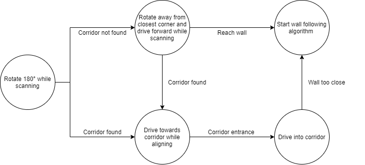
In the figure presented on the right, one can visualize the state machine after which the robot behavior is created for the Escape Room Challenge. PICO starts by scanning its environment while turning a maximum of 180 degrees. Since PICO has a viewing range of 4 rad, corresponding to approximately 230 degrees, turning 180 degrees will result in a visualization of the entire environment. If during this rotation the corridor is detected, the middle of the corridor is set as a target. PICO will start driving toward the target, while continuously scanning and aligning with the middle of the corridor. Therefore, PICO will already be fully aligned with the entrance of the corridor upon arrival and it can simply drive into the corridor. If PICO gets too close to a wall in the corridor it will start following the wall algorithm. The wall algorithm will first align the robot with the closest wall and it will start driving alongside this wall. PICO only turns if it encounters a corner or another corridor. Also, it will continuously correct its position relative to the wall, meaning that if the detected wall is not entirely perpendicular to the robot's front direction, it will adjust its position accordingly. If PICO does not find a corridor during the initial scanning procedure, it will rotate away from the closest corner and start driving forward. While driving PICO keeps scanning and if it detects a corridor it will target the middle of the corridor and follow the same process described above. In the unfortunate case PICO reaches a wall, without detecting a corridor, it will start following the previously described wall algorithm.
Corridor detection
In the escape room challenge, the only goal is to detect a corridor and drive through it. With this in mind, obstacle detection and the orientation are not considered relevant for this specific challenge. The software should be able to:
- Divide the LRF data into data segments.
- Fit lines through the segments.
- Use these lines to compute edges and corners.
- Determine target positions.
Data segmentation
1. Wall Detection
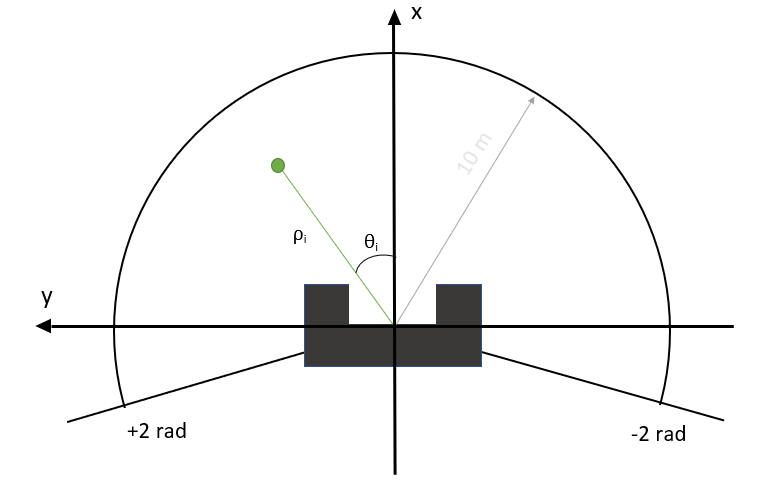
First, distances outside the range of the LRF, corresponding to 0.1 - 10m, are removed. The remaining data point are transformed from polar to cartesian coordinates using:
where ρi is the distance between PICO and an obstacle, θi is the angle of the obstacle with regard to the robot, θmin=-2 radians and is the lowest angle that can be measured, and i is the number of increments (0 to 999) where each increment is of size 4/1000.
The data segmentation is done using the split and merge algorithm. This algorithm can be used to detect line segments, which in this case represent the wall. The first step is data segmentation:
- The indices of the first and last data point resulting from the LRF data are used as i_start and i_end.
- Calculate the perpendicular distance from a line from i_start to i_end using:
- Find the maximum distance calculated in step 2 and its corresponding index.
- If the distance is above a certain threshold: split the line. Now recursively go back to step 2 for both the segments before and after the index corresponding to the maximum distance. Keep repeating this process until all i_start and the used index in step 2 are adjacent.
- If the distance is below a certain threshold: a line is found. Save the current i_start and i_end.
After all the segments are found a line is drawn between the start and the end points of each individual segment. These lines can now be used for the computations of edges and corners.
2. Corridor and edge detection
As previously mentioned, in the Escape Room Challenge, one is faced with one room with one corridor. It is therefore key to classify the angles between two line segments as either convex or concave. In case the angle is concave PICO recognizes this as a corner and if it is convex it is classified as an edge. The two points which are the most convex are assumed to be the edges of the corridor. The target position is placed in the middle of these, i.e. it is assumed to be the entrance of the corridor. Worth noticing is that PICO keeps scanning while driving towards the previously set target, if it finds a more suitable corridor edge the target will be recalculated.
Results of the Escape Room Challenge
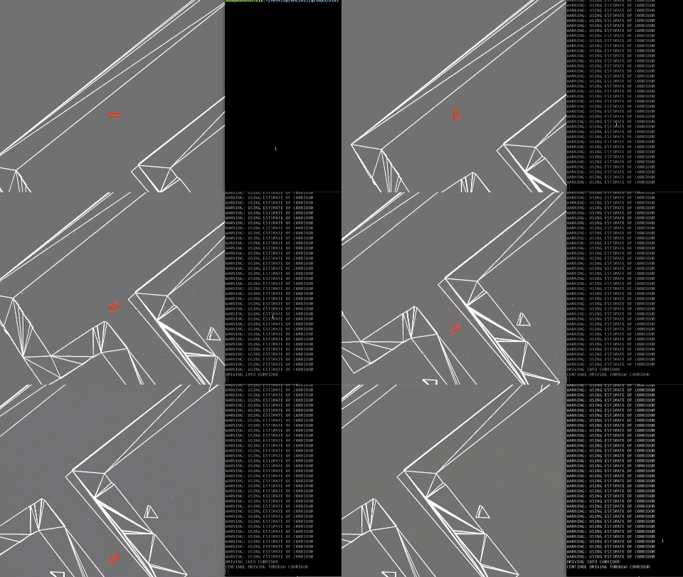
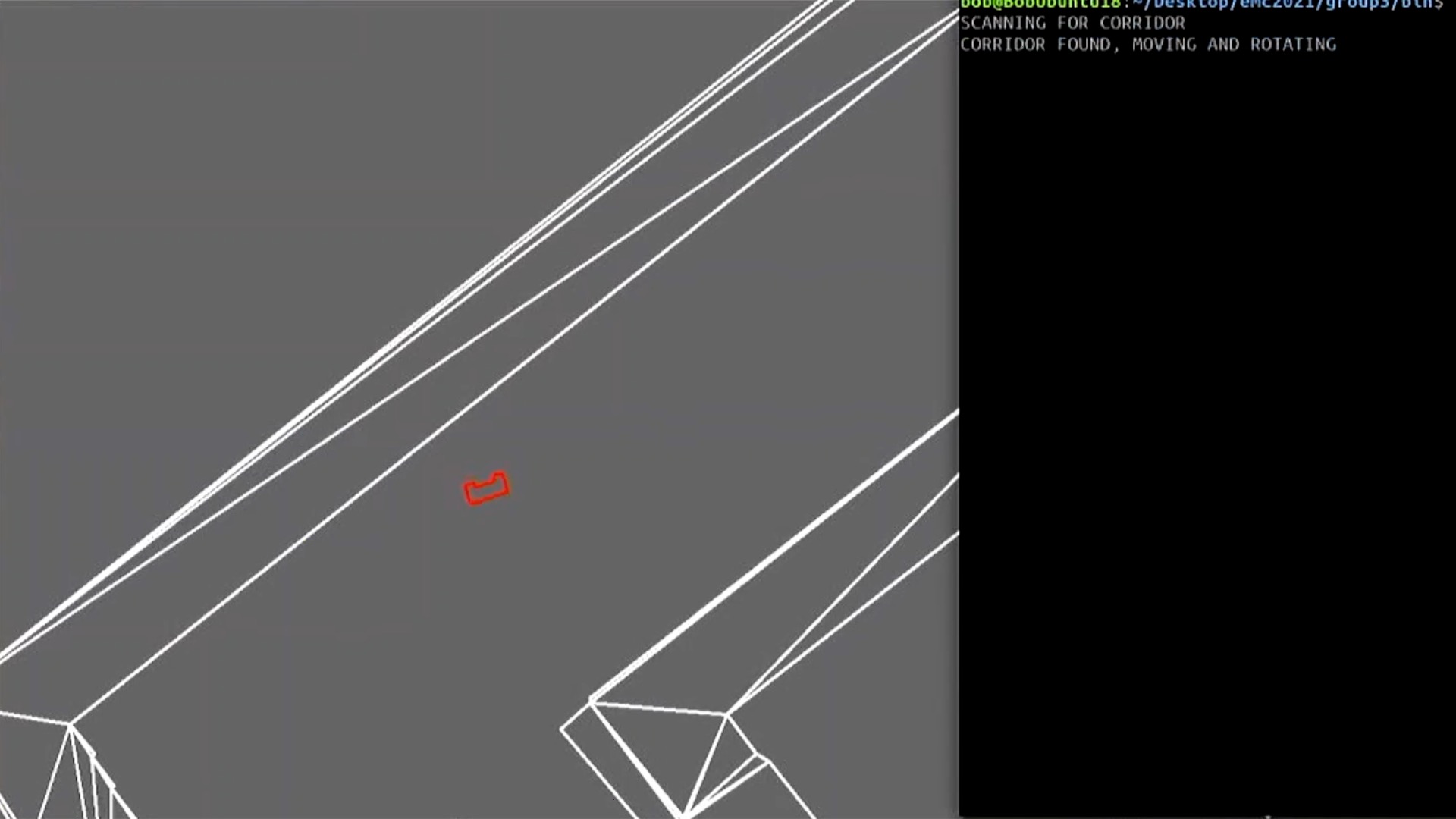
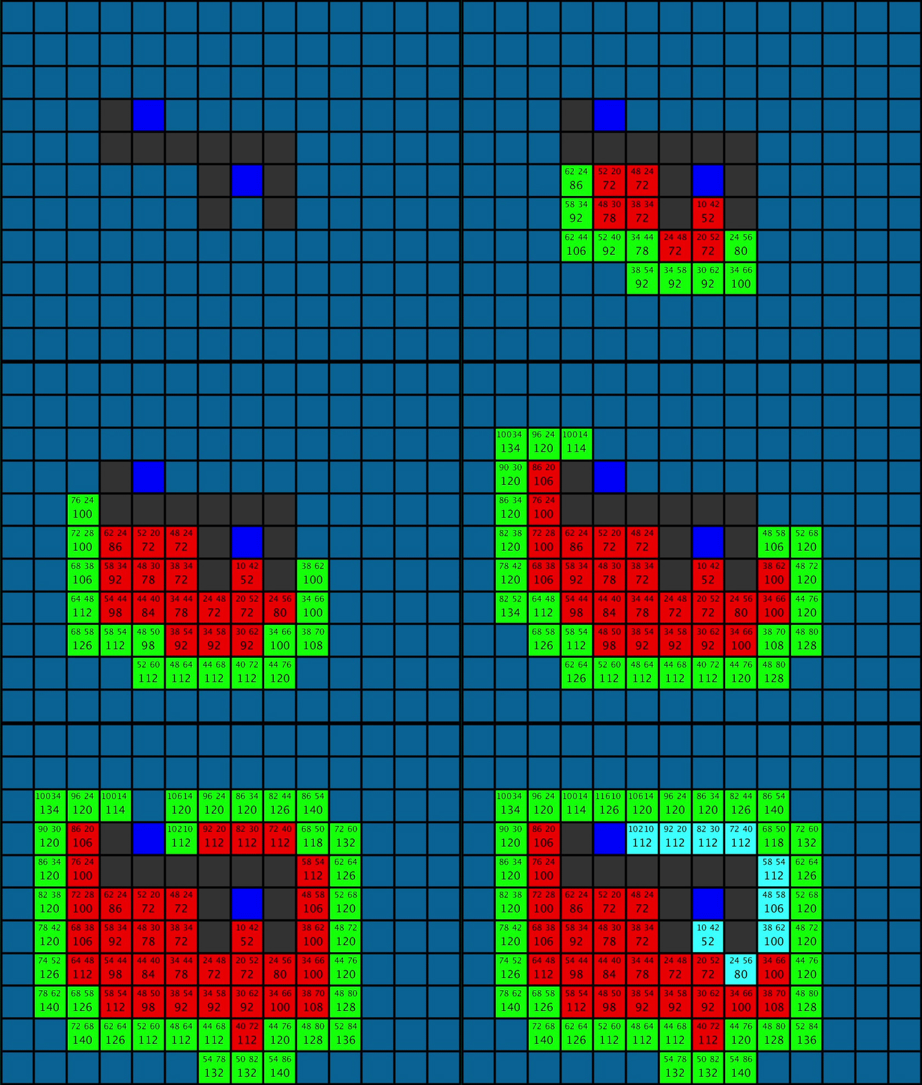
On May 12th 2021, all groups of the course 4SC020 Mobile Robot Control performed their fastest and/or most reliable version of how a PICO robot should exit a room through the only corridor present. Figure 3 shows the execution of the Escape Room Challenge by Group 3. As can be seen, the corridor through which the PICO needs to leave to finish is behind it. At the start, the robot turns counterclockwise to scan for the angles indicating a corridor. However, as can be seen more clearly in Figure 4, the robot thinks it has found a corridor right from the start. Though, this is actually not the case considering the corridor is outside of the LRF's field of view at that point in time. What PICO has found are the angles on the wall to the bottom left of the robot. It drives towards that, but since PICO is programmed to keep on scanning its surroundings, it is able to correct itself when it finds the sharper angles of the actual corridor. Following this, it aligns itself with the entrance of the corridor before driving towards the exit. Considering PICO is able to align itself with the middle of the entrance of the corridor, it can simply drive straight to the corridor. Moreover, because the corridor itself is not particularly narrow, PICO does not have to align itself with one of its walls.
Following the prerequisites, during this execution, PICO did not:
- bump into any walls
- stop moving after the start of the trial
- spend more than 5 minutes inside the room
What's more, Group 3 has completed this challenge in one try in approximately 13 seconds using the Risky Algorithm. With this time, Group 3 is the fastest of all groups and wins the Escape Room Challenge 2021 and has, thereby, successfully completed the first major milestone of the project. While this first algorithm was successful, a more safe algorithm was also provided as a back-up.
-
Figure 3: The execution of the Escape Room Challenge by Group 3.
-
Figure 4: Corridor 'found' at the start.
Hospital Challenge
Path Planning
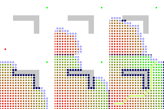
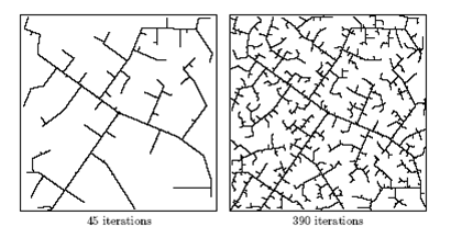
For the robot to reach every cabinet in a specified order it needs to know how to get from one cabinet to the next. Here path planning comes to the rescue. For the path planning different algorithms were investigated. One of the simplest path planning algorithms is Dijkstra's algorithms. This method starts from a initial vertex and calculates for all its surrounding neighbors the costs to get there. Sequentially are for all the neighbors the costs for their neighbors calculated and so on. This process is visualized in x . A drawback of this method is that a lot of costs are computed which are not needed, which makes the process computationally expensive. An improvement of the Dijkstra algorithm is the A* algorithm. In the A* algorithm a priority is given to nodes which have a lower distance to the goal than others. Both methods are represented in x. The A* method can become computationally expensive when there are e.g. high dimensions. This problem can be solved by using the rapidly-exploring random threes(RRT) algorithm. RRT randomly creates points and connects those to the nearest available node. Iteratively more nodes and thus more specific paths are generated. However, RRT by itself is most of the time not sufficient and an extra path planning algorithm is needed. Since for the hospital challenge the path planning should be quick and there is no indication for high dimension, the A* algorithm is used.
-
Figure X: Dijkstra's algorithm
-
Figure X: A* algorithm
-
Figure X:The RRT algorithm
The A* algorithm applied will be grid based, meaning the global map will be transferred into a grid. In this grid a path needs to be planned between a starting node and a goal node. The algorithm starts from a starting node. I then computes for each surrounding node the G-cost, which is the distance from the starting node. Also the heuristic(H) cost is calculated, which is the distance to the end node. The total cost can then be simply calculated by adding the G and H cost. The algorithm then goes to the surrounding cell with the lowest total cost and for this node it evaluates all the surrounding nodes in a similar fashion. The node which is visited is then added to the closed list, to ensure the algorithm only visit each node once. All the evaluated surrounding nodes which are not yet visited are added to the open list, so the node with the lowest cost can be found easily if needed. Grid points with obstacles are placed in the closed list, so they will not be evaluated by the algorithm. I there are multiple nodes with the same total cost the one with the lowest H-cost (so closest to the goal) is picked. If there are multiple, one will be randomly picked. When the total costs of the surrounding cells start increasing the path is no longer the cheapest. The list with open nodes will then be scanned for the node with the lowest total cost and from this node the process will start again. In case the robot is enclosed with objects and thus no path can be found, the program will automatically exit the path planning while indicating that no path could be found. The visualization of our implemented A* algorithm can be seen in figure x
-
Figure X: A* algorithm
Task Division
In order to show on what task each student from the group is, or was, working on, we made this Excel table in which every student entered their participation on a certain task. Please note that this table is often updated.
If there is a need for updating or just visualizing the current state of the table, please access the following link: [Task division.]
Everyone in this group has editing right and everyone else has just viewing right to the excel under the link found above.
