Mobile Robot Control 2020 Group 2: Difference between revisions
| (18 intermediate revisions by 2 users not shown) | |||
| Line 14: | Line 14: | ||
Bjorn Walk - 0964797 | Bjorn Walk - 0964797 | ||
== Introduction == | == Introduction == | ||
| Line 199: | Line 197: | ||
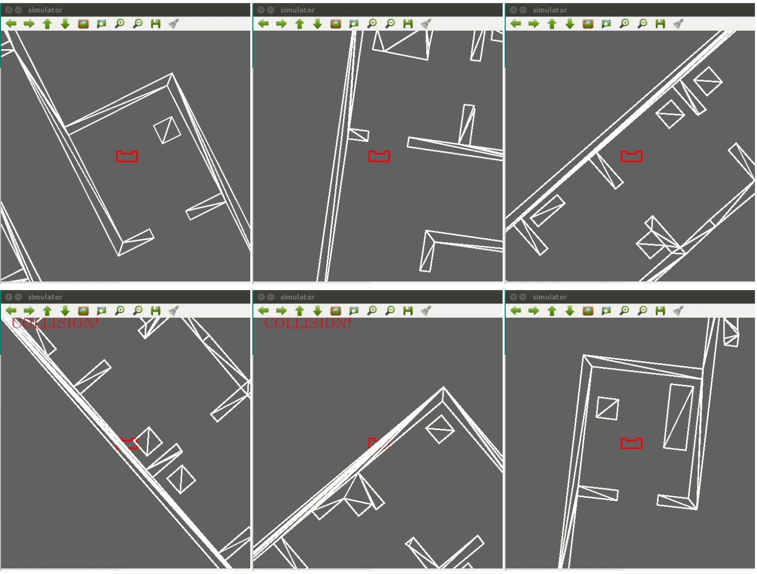
For feature extraction, the choice was made to go for corner extraction. This option was chosen for its simplicity combined with the split and merge function. Since the laser data is already segmented at the very start of the split and merge procedure, the segments the code starts with are separated walls. When the code decides to split up one of these segments once more, this indicates a corner at the location of the split. The locations of these intermediates splits are then stored in an intermediate vector. At the end of the code the actual vectors are created that contain the information about the walls, points and corners. Just before this part of the code, the found points are analyzed. When two points are close together, they are considered to be the same point. This is done to prevent the code form detecting small gaps in the walls or false point detections. When these false points are deleted, the corners are identified and stored in the world model. | For feature extraction, the choice was made to go for corner extraction. This option was chosen for its simplicity combined with the split and merge function. Since the laser data is already segmented at the very start of the split and merge procedure, the segments the code starts with are separated walls. When the code decides to split up one of these segments once more, this indicates a corner at the location of the split. The locations of these intermediates splits are then stored in an intermediate vector. At the end of the code the actual vectors are created that contain the information about the walls, points and corners. Just before this part of the code, the found points are analyzed. When two points are close together, they are considered to be the same point. This is done to prevent the code form detecting small gaps in the walls or false point detections. When these false points are deleted, the corners are identified and stored in the world model. | ||
The first draft of the localization algorithm, corner matching, uses these extracted corners. The corners extracted from the LRF are given to the algorithm in local coordinates, so with respect to the robot. The coordinates of the actual corners of the map are stored before hand in a separate file. These coordinates are defined with respect to the global map frame. These coordinates are first transformed to local coordinates for the robot using the current estimation of the pose. The global coordinates are transformed using a standard transformation matrix. The known corners of the map in local coordinates are now compared to the corner coordinates extracted using the split and merge algorithm. The algorithm finds the known corner that is closest to a found corner. This is done for every found corner. If the distance between the known corner and the found corner is larger than a certain treshold, the match is discarded as the results would be too inaccurate. If the distance is small enough, the match is stored. When only one match is found, the algorithm can not continue as it relies on having at least two comparison points available. With only one corner available, the transformation can not be identified as the single possible solution. When two or more corners are found, lines are drawn between two adjacent corners. The line between the known corners and the found corners are compared to identify the rotation of the robot with respect to the current estimated rotation. This is done for all the lines, and the mean is taken. If one of the found rotations deviates too much from the others, it is discarded since it is likely that it is wrong. When the rotation is found, the coordinates of the found corners are transformed by a purely rotational transformation matrix over this angle. Now the translational difference for each match of found and known corners can be calculated. Again the mean is taken and if a value deviates too much it is discarded. With this translational difference, the total difference between the current estimated pose and the actual pose is identified. Adding the two together gives the actual pose. This method is not very accurate as it assumes perfect data from the LRF, and only adjusts for inaccuracies in the odometry data. What has also been noticed during testing, is that the difference between the corners can be quite large even with only small rotations. This means that quite often a lot of found matches between corners are discarded due to this distance. In essence this means that the localization, although running live at 20Hz, does not actually adjust the current estimation of the pose at this rate. A next step would be to implement the Kalman filter which takes into account uncertainties in the laser data as well as the odometry data. | |||
| Line 246: | Line 244: | ||
=== Detecting closed doors === | === Detecting closed doors === | ||
Current location estimated from localization is used to determine whether PICO is close to an exit. A function near_door(double x, double y) takes estimated location as an input, compares it with location of all doors and returns the number of the nearest door(if in range). | In the Bitmap, nodes surrounding the door are blocked in a pattern that limits the robot to go through a door only in a straight-line path. This means PICO is always facing the door while approaching and passing through it. | ||
Current location estimated from localization is used to determine whether PICO is close to an exit. A function <code>near_door(double x, double y);</code> takes estimated location as an input, compares it with location of all doors and returns the number of the nearest door(if in range). | |||
When a nearest door is detected, robot checks if there is an obstruction closer than 45cm in its front. Only the frontal sector of 10 degrees of the laser data from the laser range finder is considered. In case of an obstruction, a call is made to the function <code>block_door(int door);</code> to block the corresponding door in the Bitmap. | |||
After the modification of Bitmap, path planning recalculates the path, adopting and alternative route to the cabinet. It should be noted that this method makes the door permanently inaccessible. Look at [https://gitlab.tue.nl/MRC2020/group2/-/blob/master/snippets/detection_snippet.cpp Code snippet] for Detection for more details. | |||
=== Nearby Objects === | |||
[[File:object.png|600px|thumb|center|Adaptation by path planning for objects]] | |||
For object detection, PICO actively searches area within a radius of 50cm from its current location. Whenever an object enters within this perimeter, list of all the data points are stored and first transformed to coordinates in robot frame of reference and then to global coordinates. Using the function | For object detection, PICO actively searches area within a radius of 50cm from its current location. Whenever an object enters within this perimeter, list of all the data points are stored and first transformed to coordinates in robot frame of reference and then to global coordinates. Using the function <code>coordinates2nearestindex</code>, these coordinates are converted to find corresponding nodes on the Bitmap. List of these nodes is stored and passed through the <code>block_nodes(int row, int col);</code> function. | ||
This method of object avoidance works in the principle of making nodes permanently inaccessible. Consequently, it is not robust against dynamic objects. Thus, the search radius for object detection is limited to 50cm only. | This method of object avoidance works in the principle of making nodes permanently inaccessible. Consequently, it is not robust against dynamic objects. Thus, the search radius for object detection is limited to 50cm only. | ||
| Line 298: | Line 299: | ||
*Split and Merge: [https://gitlab.tue.nl/MRC2020/group2/snippets/630 Split and Merge] | *Split and Merge: [https://gitlab.tue.nl/MRC2020/group2/snippets/630 Split and Merge] | ||
*Object Detection: [https://gitlab.tue.nl/MRC2020/group2/snippets/ | *Object Detection: [https://gitlab.tue.nl/MRC2020/group2/-/blob/master/snippets/detection_snippet.cpp Object Detection] | ||
*Path planning: [https://gitlab.tue.nl/MRC2020/group2/snippets/633 Path planning] | *Path planning: [https://gitlab.tue.nl/MRC2020/group2/snippets/633 Path planning] | ||
Latest revision as of 13:08, 2 September 2020
Mobile Robot Control 2020 Group 2
Group members
Marzhan Baubekova - 1426311
Spyros Chatzizacharias - 1467751
Arjun Menaria - 1419684
Joey Verdonschot - 0893516
Bjorn Walk - 0964797
Introduction
This is the wiki page of the Group 2 of the Mobile Robot Control course of 2020. The page contains all the information regarding the assignments accomplished within the course including the plan, procedure, algorithms, implementation and results. During the course we have been introduced to a software design and how to apply this in the context of autonomous robots. There are two assignments, which are done and reported here, namely Escape Room challenge and Hospital challenge. Unfortunately, due to the circumstances caused by the Corona virus, we were unable to apply the software on real robot, however, the simulation was adapted by the tutors to the real-life environment as much as possible.
The first task was to develop a design document which is the first step in the software development and requires the understanding of the problem, evaluation of the robot specifications and its environment, and software components. Next, from the document we proceeded to the implementation of the software for the Escape Room Challenge. After successful accomplishment of the first challenge, we moved to the design of the software for the Hospital Challenge. Finally, the results are evaluated and conclusions are drawn.
Design Document
The design document for the escape room challenge can be found here:
File:Mobile Robot Control Design Document Group2.pdf
Escape Room Challenge
The goal of the escape room challenge is to find the exit of a room autonomously and 'escape' the room through the exit corridor without bumping into the walls. In this challenge the robot is placed in a rectangular room, which dimensions as well as the initial position of the robot in the room are not known. In order for the robot to succeed in this challenge, a design document was created first, which includes the requirements & specifications, components, functions and interfaces.
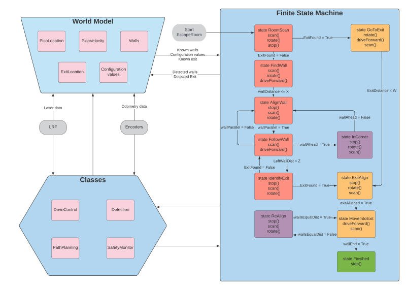
As stated in the design document, the software of the robot is developed based on a finite state machine. The finite state machine will start in a predefined initial state and will go to next states if certain conditions are met. The finite state machine will follow the states until the final state is 'finished'. While going through these states, the robot communicates with the world model. The main functions of the world model are to store important information and to share it between all classes.The information stored in the world model is for example the direction of the exit when identified or the distance to a wall. The other classes determine the actual actions of the robot. The SafetyMonitor will retrieve for example the distance to a wall and determine if the distance is larger than a certain threshold. If the wall is too close, the SafetyMonitor will tell the robot to move away from the wall to get some clearance. The detection class retrieves the laser data and determines the distances to walls or finds the exit. These parameters are then stored in the world model. Drive control determines the movement of the robot. Path planning is not used in the escape room but will be used for the hospital challenge.
At the start of the escape room challenge the robot will start to scan the room. This scan is then analyzed to determine if the exit can be seen. If the exit is detected, the robot will move in the direction of that exit until it gets close to the exit. If the exit can not be seen, the robot will rotate approximately 180 degrees to do a second scan. If the exit is detected now, the robot will move as it would if during the first scan a exit was detected. If in the second scan the exit can still not be identified, the robot will move to the closest wall found in both scans and start to follow this wall using a wall following algorithm.
When the exit is found from one of the initial scans, the robot will rotate to face the correct direction towards the exit. It will then start to move forward towards the exit. When it gets close to a wall the robot assumes it is near the exit and starts the exit alignment procedure. This exit alignment procedure makes sure that the robot will enter the hallway approximately in the middle to stay clear of the walls. When the alignment is done the robot will start the exit entering procedure.
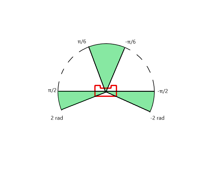
The wall following algorithm makes the robot move in a clockwise direction. When it gets close to a corner it will rotate approximately 90 degrees and use the wall to the left to correct and align to an almost perfect 90 degrees. When it suddenly sees a jump in the distance of the wall to the left, it detects this as the exit. The robot scans a larger part of the wall while driving to identify this gap. This also means that if it is only a small slit in the wall, it will not detect this slit as a exit. When the robot has then moved forward so that it is standing in front of the gap, it will rotate to face the gap. It will then align so that it is standing approximately in the middle of the gap and start the exit entering procedure.
The exit entering procedure makes sure the robot slowly drives forward until it is somewhat into the hallway. While it is doing this, it is scanning for walls to the left and right of the robot to make sure it will not hit any walls. If the robot gets to far out of the middle line of the hallway, it will reposition itself towards the middle. While in the hallway the procedure is quite similar with respect to aligning to the middle line of the hallway. In the hallway the robot will also align to be parallel to the left wall of the hallway. This is done to make sure the robot can not get to close to this wall. Combined with staying in the middle line of the hallway, this ensures that the robot will not hit any of the walls in the hallway.
While in the hallway the robot will also scan ahead slightly to the left and right. This is done to determine when the robot has crossed the finish line. When the robot no longer sees walls in the front left and right direction, it will assume that it has crossed the finish line.
A flow chart of finite state machine is shown below:
In the live Escape Room challenge the robot did not finish. In the first attempt this was due to the fact that the robot started close t0 the wall. This scenario was unfortunately not tested. The robot starts by scanning the room and trying to find the exit. When an exit is found the robot moves towards it. However, the criteria for the robot to determine that it was close to the exit was if a wall is nearby. This criteria works if the robot starts cleared of the walls and can drive straight to the exit. Since the robot started close to a wall in the challenge, it immediately thought it was at the exit and tried to align with the hallway. This obviously did not work since there was no hallway.
The second attempt was a simple wall following algorithm. However, again a specific case was not tested making the robot still not finish the challenge. In this case it was the situation where the exit was very close to a corner. When the robot gets to a corner it is supposed to rotate approximately 90 degrees, and then use the wall to the left to align with the wall. Now that the exit was close to the corner, it could not detect the wall to align with, and the software got stuck in a loop.
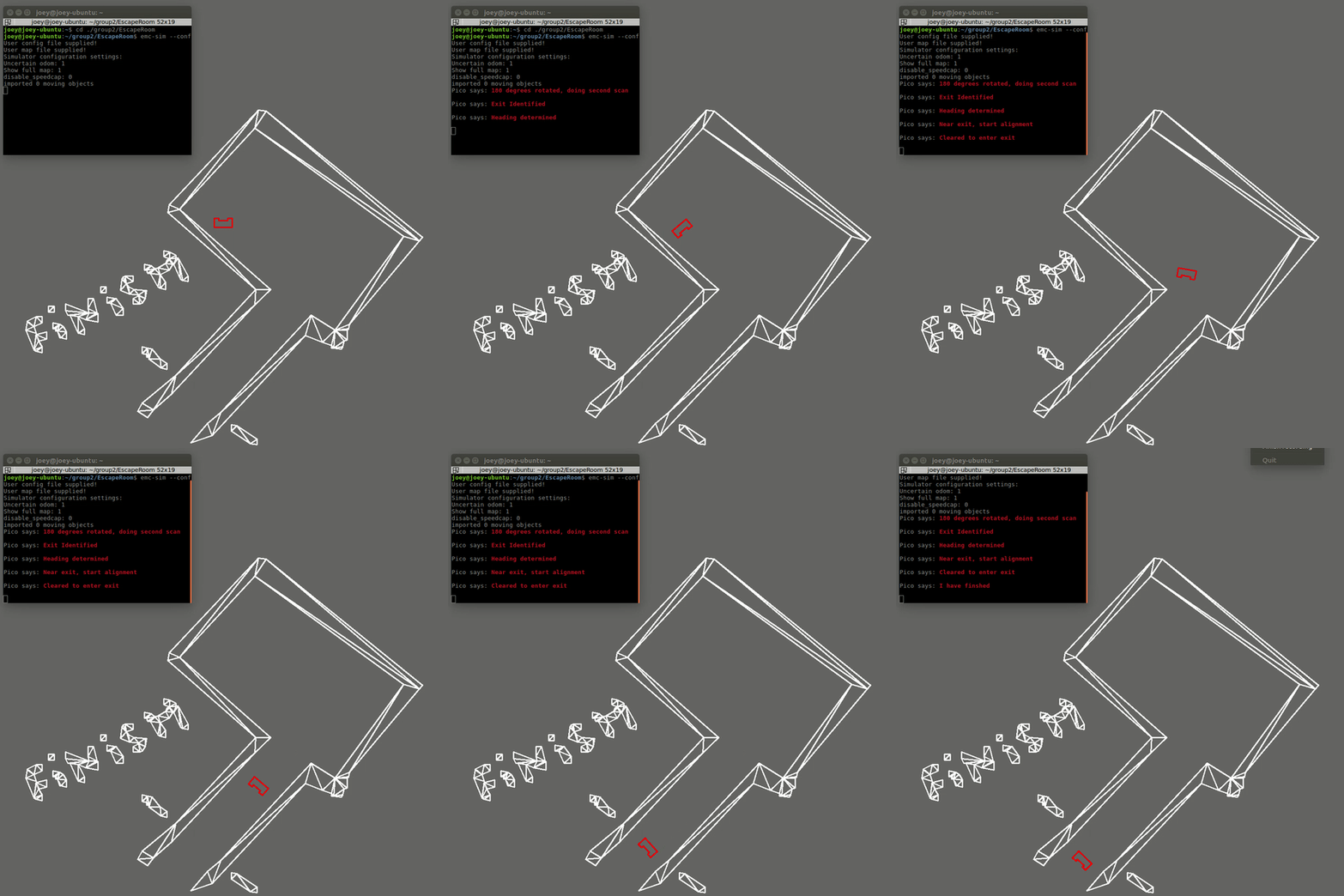
The first code was fixed by changing the criteria for when the robot assumes it is close to the exit. Now the distance to the exit is measured at the 20Hz sampling rate. This distance was already calculated in the original code, however it was not stored and used. Now that it is used, the robot will only start the alignment procedure for the hallway when this distance is below a threshold. The robot will also move away from the wall slightly after the scanning to ensure safety margins. This was already in the code, but was not executed since the robot never started moving but immediately thought it was at the exit. The result is now that the robot escapes the room in 19 seconds and stops right after crossing the finish line and speaks "I have finished". The result is shown below:
Hospital Challenge
Software Architecture Overview
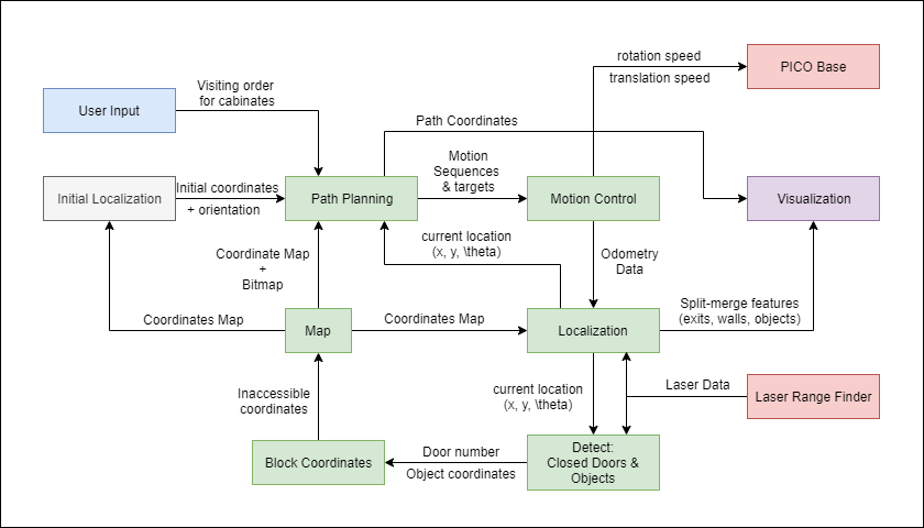
To solve the hospital challenge a schematic overview of the software architecture is created, which can be observed in the figure above. The order of visiting the cabinets, the (bit and coordinate) map and the initial localization provide the necessary input for the path planning to create a path to a cabinet. This component controls the motion control, which controls the PICO robot to get there. Whilst following the path, the real time localization keeps track of the current position and orientation of the PICO robot in the global map. With this data a feedback loop is created to the path planning, to adjust its position or to signal that a cabinet is reached. The location feedback is also used by the detection, which detects objects and closed doors, which then blocks coordinates in the map occupied by these elements, which is used by the path planning and the path is adjusted accordingly. Finally, the path planning and localization are real time visualized to analyze the performance of these algorithms.
Path Planning
The path planning is an essential component in this challenge. This component links the current position and orientation in the global map to the destination: cabinets. On its path, this component has to deal with static and dynamic objects and closed doors.
Algorithm selection
For the selection of the algorithm used for path planning, several algorithms have been considered: A*, Dijkstra, Rapidly-exploring random tree, wall following, wave propagation and Potential field algorithm. Each of these algorithms has its pros and cons, so they have been evaluated at several criteria that were relevant for the hospital challenge. This trade-off is presented in the table below.
The first 2 criteria are closely related. The speed of the algorithm is important, as hardware performance is limited. The ‘speed’ column contains some notes of the method of the algorithm. The compute index quantifies this criteria to compare it, as the speed criteria is relatively important. The compute index is based around A* which is given an index number of 100. The walls and Dijkstra compute indices are an educated guess. The others are based on the amount of nodes used in a study. The others are based on the amount of nodes used in a study. In the robustness criteria the algorithms are evaluated whether or not it can find a path at all. Path smoothness is important, as too many sharp turns can introduce a drifting error in the orientation in case of odometry feedback. It also influences the speed of the PICO robot, as it may need to stop to rotate. The implementation criteria evaluates the convenience of implementation. All team members have experience with some algorithms already, which accelerates implementation and unfamiliar algorithms can introduce implementation challenges due to the novelty factor. The implementation can also be hard, regardless of previous knowledge in case the algorithm needs to account for a large number of situations/cases.
Based on these criteria, the A* algorithm is selected. It is not the fastest, yet relatively fast. Its path is relatively smooth. Experience with this algorithm makes the implementation less complicated
| Algorithm | Compute index | Speed | Robustness | Path smoothness | Implementation | General notes |
|---|---|---|---|---|---|---|
| A* | 100 | +fast, +direct (it does not explore all the space) | +finds descent short path if it exists | -+relatively smooth, depends on grid and allowed movements | + known method | path update when obstacle detected |
| Rapidly-exploring random tree | 100 | -expands in all the space | +finds shortest path if it exists | +relatively smooth | -unknown method | good with dynamic objects |
| Potential field algorithm | 40 | -fails in case of local minimum | +relatively smooth | -unknown method | ||
| Dijkstra | 100 or higher | -slower than A*, -expands in all the space | +finds shortest path if it exists | -+ relatively smooth, depends on grid and allowed movements | + known method | path update when obstacle detected |
| Wall following | 100000 | -slow | - prone to fail in case of blocking objects | -smooth, but discontinuities exist | - difficult with many cases to account for | copy parts from escape room challenge |
| Wave propagation | 100 or higher | expands in all the space | +finds shortest path if it exists | + relatively smooth | +similar to A* | path update when obstacle detected |
Implementation
The A* algorithm is based on an existing algorithm which has been modified. An import factor in the A* algorithm is the heuristic and a well selected heuristic ensures performance and efficiency. The default heuristic in the used algorithm is the Euclidean norm with respect to the destination. With 8 movements possible from each node (diagonal,left,right,front back movement), this is not the fasted, according to a article on heuristics. A diagonal heuristic is more suitable for these allowed movements.
The algorithm uses a binary regular grid map. In parallel a regular coordinate grid map has been developed to represent the global map of the hospital. The initial position and orientation is unknown and follows from the initial localization. It may be that it does start on a node and/or is not aligned with the path that the A* algorithm gives. To account for this the path is ‘extended’ in case it is not within 25 mm radius of a node. As the map has a regular sized grid, it evaluated multiple close nodes , in case it does not start on a node. Then it selects the path of the closest node which gives the shortest path to the destination. In this code snippet this function is given. Subsequently, if needed, extra rotation is applied to align with the path. Additionally, a final orientation is applied in case the orientation of the PICO robot at the end of the path does not match the orientation of cabinet position alignment.
The grid map is illustrated in the figure below. A safety margin from the walls and cabinets of 30cm is applied in the positioning of the nodes. One can observe that there are many nodes, many of which will likely never be used. They are still present to account for any objects that might arise in the hospital challenge and require a detour using these nodes to avoid collision with objects on its path.

User interaction
The user interaction is different than mentioned in the challenge requirements to benefit the user experience. The user is asked for the input with an example and feedback is given. This benefits the user experience. The user interaction interface is illustrated in the figure below.

Motion Control
Main Control
As mentioned in the Path Planning section, path planning inputs a vector into the motion control class which contains the following information:
| Index type | Role | Stored Value |
|---|---|---|
| Even | Nature of motion | 0 for translation and 1 for rotation |
| Odd | Target for the corresponding motion | distance to travel or angle to rotate |
As this information is stored in a paired fashion inside the vector, controller searches for the even indices of the vector to determine the nature of motion and selects the corresponding translation/rotation controllers (driveForward_target and rotate_target). Values stored at the successive odd indices are used as input to the controllers.
Low-level motion control is done via class called DriveControl.cpp. Earlier functions viz. drive_forward and rotate take only speeds as inputs. Also, rotation was only possible in clockwise direction. Thus, these two functions were redesigned to take setpoints (distances and angles) as input.
Drive to Target
driveForward_target takes as input the distance (in meters) that the PICO needs to travel forward according to the path planning algorithm. At first, a fixed speed controller was implemented to move to the given goal. After a bit of research, a proportional speed controller was developed to reduce wheel slip and jerks while switching between motion behaviors (rest, in motion, in rotation). Initially, PICO starts moving its speed increases gradually as it moves away from the target and achieves its maximum speed when it has travelled half of distance to the goal. Afterwards, PICO slows down as it approaches the destination eventually coming to rest. Maximum forward movement speed is saturated to 1.5 m/s.
To keep track of the distance moved from the initial position to the new setpoint, DriveControl class stores the odometry data from the last destination and uses it as the starting position. Odometry data is acquired in real-time which corresponds to current position of PICO (odomUpdate). Using x and y coordinates the two odometry datasets as inputs in the Euclidean formula, relative distance travelled by the robot can be calculated. This distance is then compared against the input distance to define the stopping criteria.
Rotate to Target
Rotate_target takes as input the angle (in radians) that the robot needs to rotate, targetangle, and a Boolean variable, dir, that enables rotations in both, clockwise (0) and anti-clockwise (1) directions. Value for the variable dir is determined using the sign of the targetangle. Like driveForward_target, a proportional angular speed controller is present.
Angular data from odometer is discontinuous at 180° and can exhibit both increasing as well as decreasing behavior while rotating in a certain direction. Hence, it cannot be used to control the amount of rotation directly. To solve is issue, angle from the odometry data at the beginning of the rotational motion is stored in a variable called prev_angle. Current angular information can be obtained using real-time odometry information stored in odomUpdate. Using prev_angle, and odomUpdate.a, a modified variable, angle, is calculated which goes from 0 to n*π and is always increasing in anti-clockwise direction.
Finally, the variable relative_angle evaluates the difference between angle rotated and the targetangle to serve as a stopping criterion.
Localization
For successful navigation it is important that the robot is aware of its current location. In this case two different algorithm are considered for the localization, first of all Corner Matching and secondly the Extended Kalman Filter. It is worth mentioning, that both of the methods address the position tracking problem, therefore the initial position of the robot is required. Thus, before starting localization, the method for initial pose localization needs to be found.
To determine an initial pose, one can use known landmarks. In this case the door of the room where the robot starts is used. The laser data is analyzed to find the door in the same way it is done in the Escape room challenge. When the door is found, the robot will rotate to face the exact middle point of the door. This is also done to be able to determine an angle. When the robot faces the middle point, the sides of the door are found in the laser data. Using the range and the angle for these points, the x-y position can be determined using trigonometry. When the initial position is known, combined with knowing the location of the middle point of the door the robot is facing, the initial angle can be determined completing the initial estimation of the pose. The algorithm is made robust such that it can not falsely identify other objects in the room or small gaps in the walls as the door. The accuracy of the initial pose is dependent on the accuracy of the LRF. However, this initial localization is only used to get a first estimation of the pose, and the actual localization function will use this and correct it based on all the data it retrieves.
Next, the actual localization algorithm requires feature extraction and the most important features in the robot's environment are the straight lines and corners. These features are used to build a local map from laser data. To extract corners the following problem should be solved. It consists of two subproblems, namely segmentation, which deals with the number of lines and correspondence of data points to lines, and corner definition, which answers how to estimate corners from segmented lines.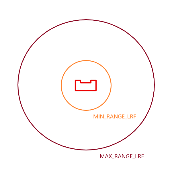
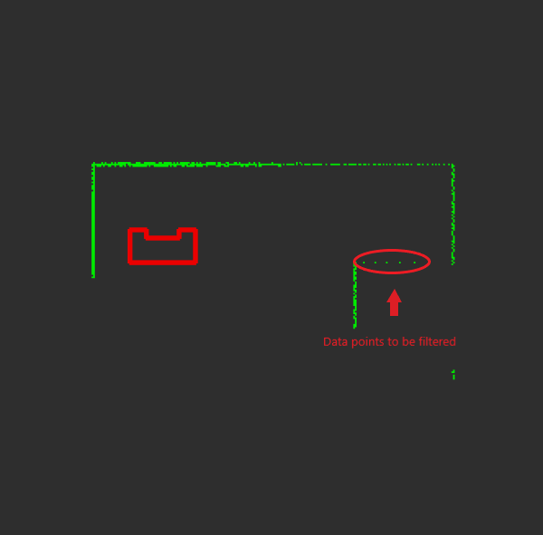
| Split and Merge Algorithm: |
|---|
| Initialize segments set S. |
| 1. Filter LRF outliers by setting thresholds MAX_RANGE_LRF and MIN_RANGE_LRF. |
| 2. Convert LRF data to cartesian coordinates. |
| 3. Calculate the distance between two cartesian points and check if it is within threshold DUMP_DIST. |
| 4. Check for a jump in LRF ranges of the filtered data set and if the jump is bigger than threshold CLUSTER_MARGIN-> make segmentation |
| Split |
| 1. Fit a line to begin and endpoint in current set S. |
| 2. Find the most distant point to the line using heron's formula. |
| 3. If distance > threshold LSE_MARGIN, then split and repeat with left and right point sets. |
| Merge |
| 1. If two consecutive segments are close/collinear enough, obtain the common line and find the most distant point. |
| 2. If distance <= threshold, merge both segments. |
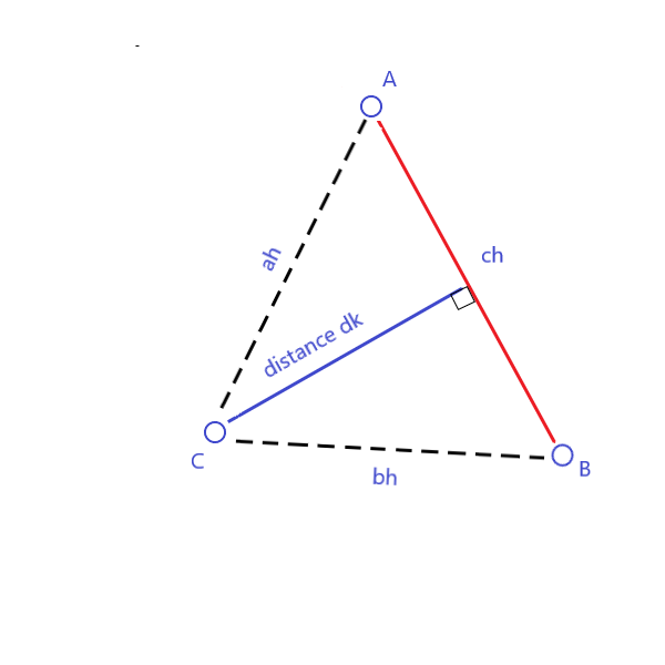

In our case the base b is ch and h is a distance-to-be-found dk. Area A is calculated by Heron's formula since all three distances ah, bh and ch can be found. To calculate area, define first

then

Finally, the distance can be calculated:

For feature extraction, the choice was made to go for corner extraction. This option was chosen for its simplicity combined with the split and merge function. Since the laser data is already segmented at the very start of the split and merge procedure, the segments the code starts with are separated walls. When the code decides to split up one of these segments once more, this indicates a corner at the location of the split. The locations of these intermediates splits are then stored in an intermediate vector. At the end of the code the actual vectors are created that contain the information about the walls, points and corners. Just before this part of the code, the found points are analyzed. When two points are close together, they are considered to be the same point. This is done to prevent the code form detecting small gaps in the walls or false point detections. When these false points are deleted, the corners are identified and stored in the world model.
The first draft of the localization algorithm, corner matching, uses these extracted corners. The corners extracted from the LRF are given to the algorithm in local coordinates, so with respect to the robot. The coordinates of the actual corners of the map are stored before hand in a separate file. These coordinates are defined with respect to the global map frame. These coordinates are first transformed to local coordinates for the robot using the current estimation of the pose. The global coordinates are transformed using a standard transformation matrix. The known corners of the map in local coordinates are now compared to the corner coordinates extracted using the split and merge algorithm. The algorithm finds the known corner that is closest to a found corner. This is done for every found corner. If the distance between the known corner and the found corner is larger than a certain treshold, the match is discarded as the results would be too inaccurate. If the distance is small enough, the match is stored. When only one match is found, the algorithm can not continue as it relies on having at least two comparison points available. With only one corner available, the transformation can not be identified as the single possible solution. When two or more corners are found, lines are drawn between two adjacent corners. The line between the known corners and the found corners are compared to identify the rotation of the robot with respect to the current estimated rotation. This is done for all the lines, and the mean is taken. If one of the found rotations deviates too much from the others, it is discarded since it is likely that it is wrong. When the rotation is found, the coordinates of the found corners are transformed by a purely rotational transformation matrix over this angle. Now the translational difference for each match of found and known corners can be calculated. Again the mean is taken and if a value deviates too much it is discarded. With this translational difference, the total difference between the current estimated pose and the actual pose is identified. Adding the two together gives the actual pose. This method is not very accurate as it assumes perfect data from the LRF, and only adjusts for inaccuracies in the odometry data. What has also been noticed during testing, is that the difference between the corners can be quite large even with only small rotations. This means that quite often a lot of found matches between corners are discarded due to this distance. In essence this means that the localization, although running live at 20Hz, does not actually adjust the current estimation of the pose at this rate. A next step would be to implement the Kalman filter which takes into account uncertainties in the laser data as well as the odometry data.
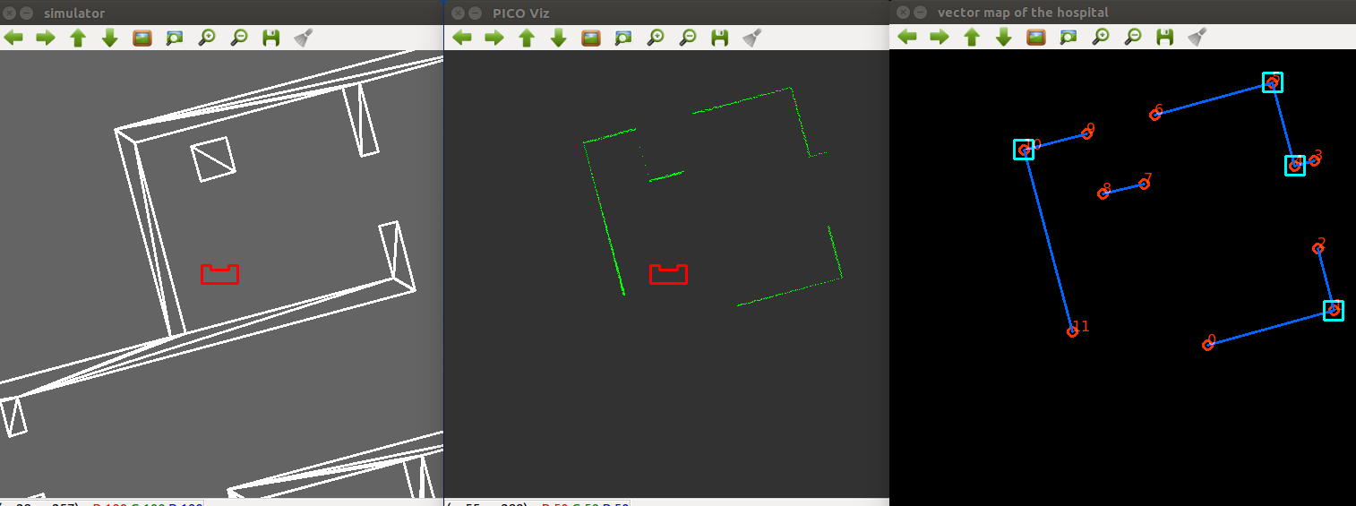
Due to the fact that corner matching localization didn't provide accurate enough position of the robot, a more robust methodology was needed. The alternative choice for localization method was the Extended Kalman Filter (EKF) because its implementation is considered easier than other methods, such as the Particle Filter and its probabilistic approach can lead to more accurate estimation than other methods, such as line segment localization. Unfortunately, due to limited amount of time the implementation of EKF did not provide robust results for localization and therefore it was not implemented in the main code for the hospital challenge. However, the method was applied and tested on a simplified example, where the real position of the robot was estimated during its movement from one known point in the map to another point. The basic steps of the EKF algorithm as implemented for the hospital challenge are described in the following paragraphs. A code sample of the simplified example is attached at the end of this wiki page.
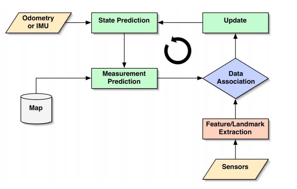
Stage prediction: For the implementation of the EKF a prior knowledge of the initial position of the robot is required (x,y and theta with respect to the global frame of the hospital map). This is provided by the initial localization module, which was described in a second paragraph of this section. The first step of the algorithm (Stage Prediction) takes into account the given initial position of the robot and it calculates a predicted position by adding the odometry data (Odometry) given by the encoders (assuming that the odometry data are accurate, without any errors). The equations for state prediction and state covariance are:
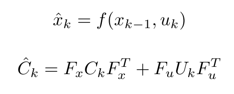
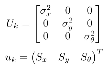
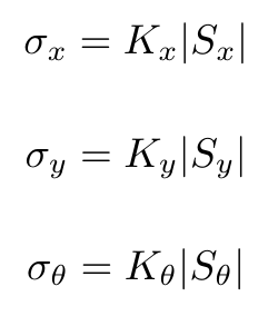
where u_k is the displacement vector and U_k the variance matrix for the inputs, given as follows:
Measurement prediction: At the measurement prediction stage the position of the the known corners with respect to the global map frame (map) are expressed with respect to the predicted position of the robot. This transformation of every known corner (i) of the map is demonstrated as the following function:

Landmark extraction:
At landmark extraction the data from the laser sensors are used in the split and merge algorithm, as described in a previous section, in order to calculate the position of the corners inside the laser range with respect to the robot frame (Cartesian coordinates). The position vector of each observed corner (j) and the observation uncertainty matrix are described as follows:

Data association: At the data association stage the observed corners from the Landmark Extraction stage are matched with the known corners from the map. The difference of the position of observed and known corners with respect to the robot frame are calculated and saved in the innovation vector v_k. For every possible match up, if the difference is smaller than a specified threshold then the observed corner is identified. If the observed corner is not matched up with any of the known corners (i.e. in the case of an unknown static or dynamic object) then the corner is ignored and the algorithm continues with testing the next possible match up. A different approach of this algorithm uses the information of the unmatched corners to identify and locate unknown objects. For the purposes of the hospital challenge this information is ignored, since the object detection is dealt with a different method. The innovation vector and the innovation covariance matrix are described as follows:
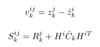
Update: At this stage of the EKF algorithm the position of the robot, the state covariance and the vector with the Kalman gains are updated. The composite innovation Vk, the composite innovation covariance Sk and the composite of the measurement prediction function H are calculated from vk_ij, Sk_ij and Hi respectively. The update equations are:
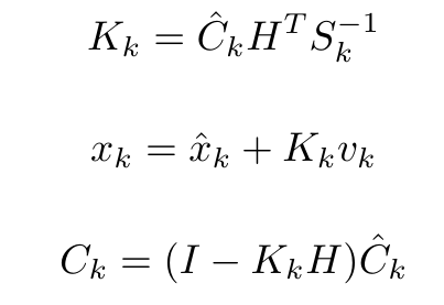
The implementation of the EKF algorithm on a simplified example, where the robot is moving from a known position to another position is attached at the end of the this wiki page.
Detection
Detection class is responsible for identifying closed doors and nearby objects.
Detecting closed doors
In the Bitmap, nodes surrounding the door are blocked in a pattern that limits the robot to go through a door only in a straight-line path. This means PICO is always facing the door while approaching and passing through it.
Current location estimated from localization is used to determine whether PICO is close to an exit. A function near_door(double x, double y); takes estimated location as an input, compares it with location of all doors and returns the number of the nearest door(if in range).
When a nearest door is detected, robot checks if there is an obstruction closer than 45cm in its front. Only the frontal sector of 10 degrees of the laser data from the laser range finder is considered. In case of an obstruction, a call is made to the function block_door(int door); to block the corresponding door in the Bitmap.
After the modification of Bitmap, path planning recalculates the path, adopting and alternative route to the cabinet. It should be noted that this method makes the door permanently inaccessible. Look at Code snippet for Detection for more details.
Nearby Objects
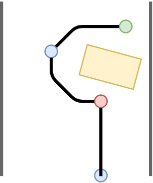
For object detection, PICO actively searches area within a radius of 50cm from its current location. Whenever an object enters within this perimeter, list of all the data points are stored and first transformed to coordinates in robot frame of reference and then to global coordinates. Using the function coordinates2nearestindex, these coordinates are converted to find corresponding nodes on the Bitmap. List of these nodes is stored and passed through the block_nodes(int row, int col); function.
This method of object avoidance works in the principle of making nodes permanently inaccessible. Consequently, it is not robust against dynamic objects. Thus, the search radius for object detection is limited to 50cm only.
Visualization
In order to debug the code in a more efficient way, the map and important functions of the code are visualized with a visualization class using the openCV library. In the beginning of the code a white canvas is created in a separate window where the map will be visualized from the provided JSON file. Then this code is extended to visualize the important functions each time these functions are called, the considered functions in this case are the pathplanning and the line & corner extraction of the robot's laserdata. Furthermore, a second window is created in which the laserdata in front of the cabinet, is visualized, as it should be saved as a different image for each cabinet.
The visualization is made using basic functions of the openCV library such as imshow() and imwrite(). Furthermore, different structures are made for each specific object such as the cabinets, walls, corners, etc, in order to visualize the correct associated data.
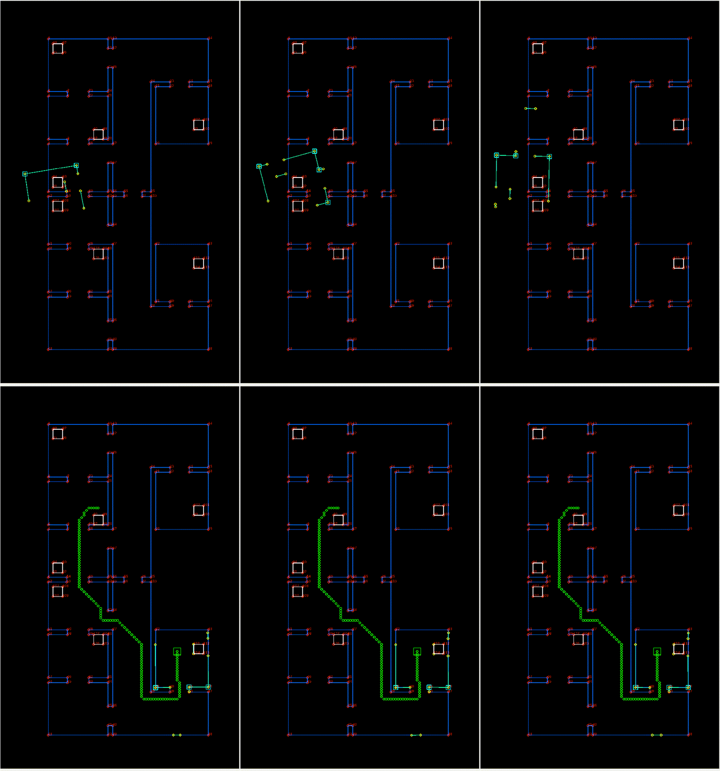
In order to save the laserdata in front of the cabinet, the following visualization function with openCV code is used to store for each cabinet a separate image
 void save_snapshots(int i)
 {
    cv::Mat image_laser;
    cv::flip(imag,image_laser,0);
    std::ostringstream name;
    name<<"cabinet_image"<<i<<".jpg";
    cv::imwrite(name.str(), image_laser);
 }
Results and Discussion
The escape room challenge showed the importance of thorough testing of the code. One small assumption made the code not function properly at the challenge. If the code was properly tested for different scenarios, this could have been prevented. Another point of interest learned from the escape room challenge was that it is important to communicate between the different teams when working on different parts of the code. After completing the separate parts of code, it took a long time to merge the code and fix bugs. This led to the limited amount of testing done. Lastly, when work started on the hospital challenge, the realization came that most of the code for the escape room challenge was not useful for the hospital challenge. When designing a code, it is good to look ahead and think of what would be useful in future endeavors instead of only looking at the current objective.
The motion picture above shows the achieved result with path planning in the published map of the hospital challenge with the correct initial position. The initial position (and orientation) was determined separate of the path planning script with the initial localization as both components work well, albeit independently. The output of the initial localization was copied to the path planning. The path planning in combination with the drive control and map, follows a trajectory with feedback from the odometry data. Ideally if the localization would have worked, the location of PICO would be corrected whilst following the path. Furthermore, the object detection would have updated the map, which path planning would have used to avoid the objects. With more time, these parts could have been merged.
The Split and Merge algorithm works well and is quite robust. It is able to detect walls and corners, which can be used for localization and visualization. It did, however, take a lot of time to get it to work accurately, which left too little time to be able to properly use the extracted data for localization. A first simple form of localization in the form of corner matching was made, but due to a limited amount of time and inexplicable errors with the encoder data, it was not tested enough to give an accurate localization.
Unsolved problems and attempts to solve them
After merging the individual components (localization and path planning) of the hospital challenge, the odometry gave errors. To be more specific, it obtained other variables' and random values. For example, the angle of the odometry has a range of -pi to pi, yet it obtained values like 4.5 which should be impossible. This odometry data is accessed by pointers, so somewhere in the written code a value is written to the odometry data, which should not happen or the odometry code, which is accessed and not written by us, accesses the wrong memory locations. In an attempt to solve this, the component where written in the same style which accesses the odometry data once per rate cycle, to eliminate incorrect writing to this variable. Unfortunately, this did not solve this issue. Besides, the code was also thoroughly checked to see whether some code writes to that pointer’s address, which was not the case. This unresolved issue had two consequences: the hospital challenge was not executed well in case the initial positioning was added to the path planning and a lot of time was spend on it, delaying other parts of the project. In case more time would have been available, the components should have been developed with more intense collaboration, which could have solved this error in the first place. In addition, some difficulties were faced during the implementation of the EKF. The sample code created for the simplified example did not always return a value for the real position of the robot and most of the times was crashing in random places all over the code. After some research the problem was located in some memory errors. Unfortunately, due to limited amount of time this problem was not solved, the EKF implementation did not give robust enough results and thus it was not included in the main code of the hospital challenge.
Code Snippets
- Split and Merge: Split and Merge
- Object Detection: Object Detection
- Path planning: Path planning
- Extended Kalman Filter: Extended Kalman Filter
Logs
| Meeting # | Date and Location | Agenda | Meeting notes |
|---|---|---|---|
| 1 |
Date: 28-04-20 Time: 10:00 Platform: MS Teams |
|
|
| 2 |
Date: 01-05-20 Time: 14:00 Platform: MS Teams |
|
|
| 3 |
Date: 05-05-20 Time: 10:00 Platform: MS Teams |
|
Work division
|
| 4 |
Date: 11-05-20 Time: 11:00 Platform: MS Teams |
|
Work division
|
| 5 |
Date: 18-05-20 Time: 11:00 Platform: MS Teams |
|
Work division
|
| 6 |
Date: 22-05-20 Time: 14:00 Platform: MS Teams |
|
Work division is the same
|
| 7 |
Date: 26-05-20 Time: 11:30 Platform: MS Teams |
|
Work division is the same
|
| 8 | Date: 29-05-20 | miscellaneous | |
| 9 | Date: 01-06-20 | miscellaneous | |
| 10 | Date: 08-06-20 | miscellaneous | |
| 11 | Date: 15-06-20 | miscellaneous | |
| 12 | Date: 19-06-20 | miscellaneous | |
| 13 | Date: 23-06-20 | miscellaneous |