Embedded Motion Control 2019 Group 1: Difference between revisions
| (197 intermediate revisions by 5 users not shown) | |||
| Line 172: | Line 172: | ||
All components communicate with the world model to ensure that they operate using the same perception of surroundings and from the same tasks. This is realized by allowing the components to perform certain tasks based on the state of the world model. For example, if the planner notices that the exit is found in the escape room challenge, the state is changed to ''ExitRoom''. The change of this state causes the controller, monitor and perceptor to only use the functions relevant to leaving the room. In this case, the functions of the controller could be ''MoveToExit'',''MoveToTrajectory'' and ''AvoidStationaryObstacle''. | All components communicate with the world model to ensure that they operate using the same perception of surroundings and from the same tasks. This is realized by allowing the components to perform certain tasks based on the state of the world model. For example, if the planner notices that the exit is found in the escape room challenge, the state is changed to ''ExitRoom''. The change of this state causes the controller, monitor and perceptor to only use the functions relevant to leaving the room. In this case, the functions of the controller could be ''MoveToExit'',''MoveToTrajectory'' and ''AvoidStationaryObstacle''. | ||
The world model thus contains the state on which the components base their events, current location with respect to a certain reference (e.g. the wall besides | The world model thus contains the state on which the components base their events, current location with respect to a certain reference (e.g. the wall besides PICO or the position within a room), landmarks currently visible and past landmarks to determine the trajectory, a desired and actual trajectory and the incoming sensor data. | ||
The planner contains both strategies for the challenges. The strategy to be used in the escaperoom challenge is illustrated below. PICO starts in the ''Orient'' state to immediately find the exit if the exit is in sight, and otherwise a wall to follow. If a wall is found, the monitor indicates this by updating the world model. The planner notices this event and sets the state of the world model to ''FollowWall''. This process continues until the state ''ObjectiveComplete'' is reached. | The planner contains both strategies for the challenges. The strategy to be used in the escaperoom challenge is illustrated below. PICO starts in the ''Orient'' state to immediately find the exit if the exit is in sight, and otherwise a wall to follow. If a wall is found, the monitor indicates this by updating the world model. The planner notices this event and sets the state of the world model to ''FollowWall''. This process continues until the state ''ObjectiveComplete'' is reached. | ||
[[File:StatemachineEscapeRoom_v2.png|center]] | [[File:StatemachineEscapeRoom_v2.png|thumb|center|upright=3|alt=The state machine for the escape room challenge.|The state machine for the escape room challenge.]] | ||
= Software Architecture = | = Software Architecture = | ||
| Line 183: | Line 183: | ||
==Summary== | ==Summary== | ||
A modular software architecture was created in which the event loop always remains the same. A plan is seen as a state machine of controllers, which are in turn state machines. These state machines can be constructed in a user friendly manner, using function pointers to prevent code duplication and to keep a clear overview of the robot's strategy. Monitors can be created in an equally modular way. Additionally, all relevant information passes through a central WorldModel. Monitors and controllers that are not relevant to the current state of the Plan state machine are not executed to spare resources. Adding semantic information such as Corners or | A modular software architecture was created in which the event loop always remains the same. A plan is seen as a state machine of controllers, which are in turn state machines. These state machines can be constructed in a user friendly manner, using function pointers to prevent code duplication and to keep a clear overview of the robot's strategy. Monitors can be created in an equally modular way. Additionally, all relevant information passes through a central WorldModel. Monitors and controllers that are not relevant to the current state of the Plan state machine are not executed to spare resources. Adding semantic information such as Corners or Checkpoints to the WorldModel is easy and scalable. | ||
== User manual == | == User manual == | ||
| Line 190: | Line 190: | ||
===Creating the concept=== | ===Creating the concept=== | ||
# Draw the plan on paper as a state machine. Give all states an ID (int), starting from zero. Give all connections (events) an ID as well, starting from zero. | # Draw the plan on paper as a state machine. Give all states an ID (int), starting from zero. Give all connections (events) an ID as well, starting from zero. | ||
# Every state of the plan corresponds to a controller. Draw each controller on paper as a state machine. Again give an ID (int) to each state. | # Every state of the plan corresponds to a controller. Draw each controller on paper as a state machine. Again give an ID (int) to each state. '''Note that the numbering is shared by all controllers, but that it is separate from the plan.''' For example, the plan can have states with IDs 0, 1, 2. These three controllers could have states with IDs (0, 1, 2, 3), (4, 5), (6, 7, 8). The same numbering rule holds for connections (events). | ||
# Every connection (event) of the plan corresponds to a monitor. Write down in pseudo-code what exactly this monitor needs to see from the WorldModel before it triggers an event. | # Every connection (event) of the plan corresponds to a monitor. Write down in pseudo-code what exactly this monitor needs to see from the WorldModel before it triggers an event. | ||
| Line 201: | Line 201: | ||
# Create the controllers in ''controllers.cpp''. Write a function such as ''ControllerCollection getTestControllers(emc::IO *io, WorldModel *wm)''. Then create the controllers as follows. | # Create the controllers in ''controllers.cpp''. Write a function such as ''ControllerCollection getTestControllers(emc::IO *io, WorldModel *wm)''. Then create the controllers as follows. | ||
## Initialize an ''std::Vector<StateMachine> controllers;''. | ## Initialize an ''std::Vector<StateMachine> controllers;''. | ||
## In | ## In '''the same order''' as the definition of the state IDs, for each controller, create a StateMachine object with its initial state ID, the amount of states and the amount of connections. | ||
## For each state in every controller, create a State object. Pass to the constructor the state ID. In addition, pass the name of a ''void(emc::IO*)'' function that you write in the same source file. This is the body that will be executed in every iteration of the event loop. For example, if the active state is 'driveBackwards', then the function body could be ''io->sendBaseReference(-1*MAX_FORWARD_SPEED,0,0);''. Lastly, pass to the constructor a pointer to an emc::IO object. Add each State object to its corresponding StateMachine object and add each StateMachine object to the vector ''controllers''. | ## For each state in every controller, create a State object. Pass to the constructor the state ID. In addition, pass the name of a ''void(emc::IO*)'' function that you write in the same source file. This is the body that will be executed in every iteration of the event loop. For example, if the active state is 'driveBackwards', then the function body could be ''io->sendBaseReference(-1*MAX_FORWARD_SPEED,0,0);''. Lastly, pass to the constructor a pointer to an emc::IO object. Add each State object to its corresponding StateMachine object and add each StateMachine object to the vector ''controllers''. | ||
## When all StateMachine objects are made, return a ControllerCollection object made from the vector of Statemachine objects, the ID of the initial controller to be active and the pointer to the WorldModel object. | ## When all StateMachine objects are made, return a ControllerCollection object made from the vector of Statemachine objects, the ID of the initial controller to be active and the pointer to the WorldModel object. | ||
| Line 209: | Line 209: | ||
## Return a MonitorCollection of the Monitor objects and the initial active monitor IDs. | ## Return a MonitorCollection of the Monitor objects and the initial active monitor IDs. | ||
## Repeat the above steps for the plan monitors in a separate function. | ## Repeat the above steps for the plan monitors in a separate function. | ||
# Integrate everything in ''main.cpp'' by simply editing the function names to the ones that you just created. The event loop does not have to be edited because of the modular design. | # Integrate everything in ''main.cpp'' by simply editing the function names to the ones that you just created. The event loop does not have to be edited because of the modular design. | ||
==Selling points of the software architecture== | |||
# The modular software structure enables a developer to test and validate software independently. | |||
# A full plan with corresponding state machines can be implemented in the sofware architecture in an intuitive manner. | |||
# Controllers and monitors can be reused indefinitely. | |||
# Only controllers and monitors relevant to the current state are executed to spare resources. | |||
# No grids or potential fields are used for path planning or route execution. | |||
# The software modules only communicate through a world model and not among each other to add context to data. | |||
# Information is interpreted semantically where possible. New information can be interpreted semantically in the world model in a easy and scalable method. | |||
# The architecture outputs a UML diagram of the implemented state machines to check if they are implemented correctly, and to troubleshoot if necessary. | |||
==Technical overview== | |||
The software architecture consists of a WorldModel object, a Perception object, a StateMachine object for the plan, a ControllerCollection object and a MonitorCollection object. Each of these components will be discussed below, starting with the main program. The simplified overview of the software architecture shown on the right is used as aid to describe the components. | |||
[[Image:SoftwareArchitecture.png |thumb|right|300px|Simplified overview of the software architecture]] | |||
#Main program: event loop. The event loop is shown in a [https://gitlab.tue.nl/EMC2019/group1/snippets/143 code snippet] in Gitlab. Everything is clearly separated and there is a clear overview of which class is doing which tasks. The controllers and monitors are loaded from a separate file, that also includes all monitor and controller functions. See the user manual above for more information. | |||
#WorldModel: This component is what brings everything together. The configure() function processes the event queue that was filled by the monitors, and switches active controllers and monitors accordingly. | |||
#Plan (StateMachine with State objects). A StateMachine object, such as the plan, contains several State objects and Connection objects that describe their relations. Each State contains a function pointer which is execution upon calling the executeBody() function. This executeBody() function can be configured to invoke either one of the controllers (which are StateMachine objects), or a function pointer supplied by the user. | |||
#Controllers: as seen in the overview, the controllers are put in a ControllerCollection object, which contains a vector of StateMachine objects and a function compute() to invoke the function body of only the active controllers. | |||
#Monitors: these work similar to the controllers, as can be seen in the overview. The function bodies that are passed to Monitor Objects have to invoke worldModel->addEvent(int event), when a certain condition is met. | |||
#Graph: the functionality of the graph is explained in more detail elsewhere. Simply put, the functions displayed in the overview show how nodes (checkpoints) can be used and where a shortest path can be generated. | |||
#Perception: this object is the only instance which is reading the laser data and odometry information. It includes the localization functionality and updates the position of PICO in the WorldModel. In addition, the OpenCV window is managed in this class. | |||
= The Escape Room Challenge = | = The Escape Room Challenge = | ||
== The simulation == | == The simulation == | ||
* | For the first challenge, we built a wall-follower combined with an exit detector. As can be seen in the simulation gif, PICO follows the wall with lazy control: PICO corrects itself only in the event that it comes too close to a wall. If PICO almost is at a wall, it rotates 90 degrees to the right, and follows the next wall. If it finds an exit, it turns left, and follows the corridor towards the finish line. | ||
[[File:ER_SIM_RESIZE.gif|thumb|center|upright=3|alt=Simulation of escape room challenge.|Simulation of escape room challenge.]] | |||
== Result of the Escape Room challenge == | |||
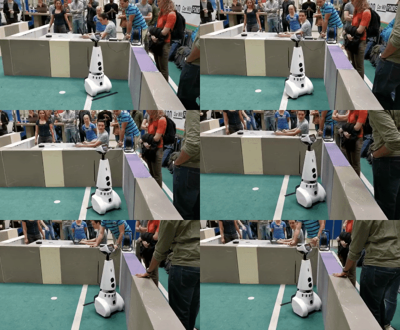
As can be seen in the gif below, during the first attempt PICO drove into the wall immediately. This has to do with the margins we set on PICO to avoid the walls, which were not set around PICO but only in front of it. Therefore, the margin was not large enough, and it drove into a wall. | |||
[[File:Escaperoomgifagain.gif|thumb|center|upright=3|alt=The first try of the escape room challenge.|The first try of the escape room challenge.]] | |||
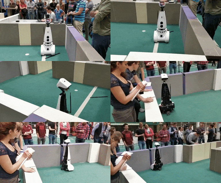
PICO was repositioned, and another try was given. During the second run, PICO drove towards the wall, and turned right when it was 0.3 meters in front of it. It then followed the wall on its left, until it found another wall in front of it. Then it turned right again, to follow the wall on its left. Due to a slight gap in the wall PICO thought it had found the exit, and turned towards it. Since this was not the actual exit, the challenge failed. | |||
[[File:escape_room_real.gif|thumb|center|upright=3|alt=The second try of the escape room challenge.|The second try of the escape room challenge.]] | |||
== Learning points Escape Room challenge== | |||
The outcome of the Escape Room Challenge itself is that the plan was not robust enough. The small gap in the wall made PICO think that the exit was found already, resulting in a collision with a wall and failing the Escape Room Challenge. The overall learning points that can be taken from this are: | |||
* The margins set on PICO should be set a bit larger, since as can be seen in the second .gif above, PICO almost bumped into one of the walls and made the 'referee' shut it down. | |||
* When defining a distance w.r.t. a wall / object, an average of a couple of data points should be taken (so a cone of points) instead of a single datapoint. This to make sure PICO will be able to cope with the real world which is never perfect. | |||
= The Hospital Challenge = | |||
== Strategy == | |||
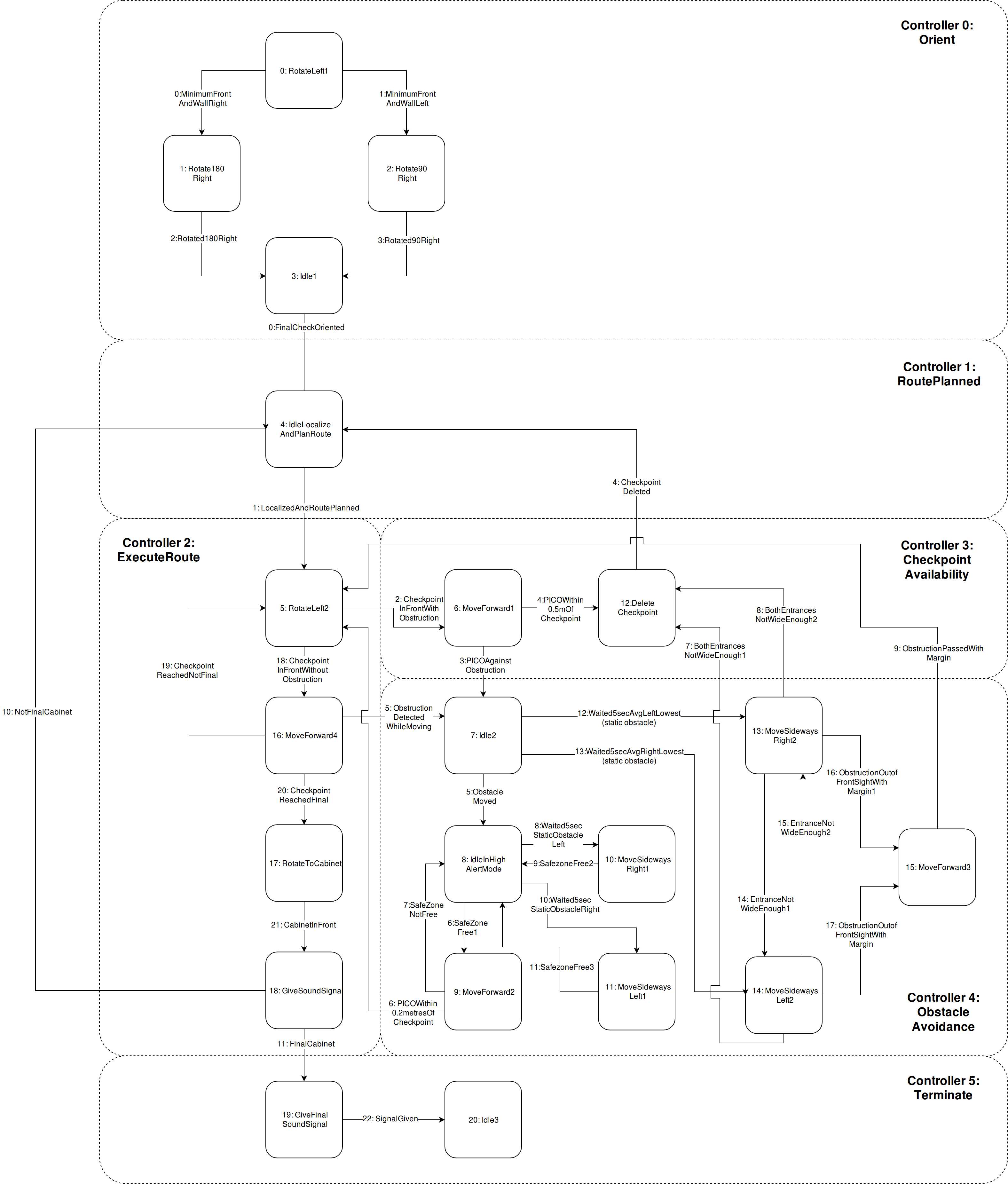
For the hospital challenge, a strategy is established consisting of 6 controllers: Orient, RoutePlanned, ExecuteRoute, CheckpointAvailability, ObstacleAvoidance and Terminate. Combining these controllers enables PICO to autonomously execute a route in which an arbitrary number of cabinets is visited. These controllers also enable PICO to function correctly for the map and its variations due to static and dynamic obstacles, and deviations in the provided map versus the real world. To convey a clear image of the hospital challenge strategy, it is illustrated in the figure at the end of this section. | |||
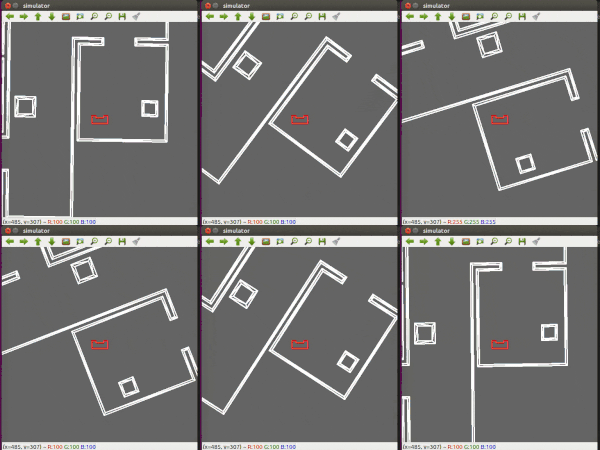
[[File:Orient_group1.gif|frame|right|An illustration of the Orient controller]] | |||
At the start of every attempt of the hospital challenge, PICO starts in the Orient state. This state functions as a calibration for PICO to position itself in the most favorable position for the localization, which is the position in which PICO is looking into the room and not to a wall or a corner. The Orient controller thus heavily depends on the conditions of the starting area of PICO in the hospital challenge. This area is given prior to the challenge and consists of an area of one square meter in which PICO can be placed arbitrarily. For this reason, four possibilities are considered: the square meter lies in the middle of a room (against no wall), against a wall, in a corner (and thus against two walls), or against three walls. In the event that the starting position does not lie against a wall, the Orient controller is redundant and thus eliminated from the strategy. For the simulations, an assumption is made that PICO will start in a corner, so the Orient controller is implemented for this case. This controller is illustrated on the right. Note that PICO starts in the correct orientation to localize in the simulation. This is, however, not a certainty in the actual challenge. For the other two possibilities, only a state machine has been established. Fortunately, the starting area of PICO for the final challenge indeed lay in a corner, meaning that no other Orient controller had to be implemented. | |||
Once PICO is oriented, PICO switches to the Localize controller. The exact algorithm applied by PICO to localize is explained in the section 'Localization'. When PICO has localized itself, it plans a route based on its current position, the position of the cabinet it has to visit next, and all the checkpoints in between. The checkpoints are visualized as the green dots in the [http://cstwiki.wtb.tue.nl/index.php?title=Embedded_Motion_Control_2019_Group_1#Test_map Test Map]. In case multiple routes are possible, e.g. due to the fact that a room has multiple doors through which PICO can enter, PICO picks the route with the least amount of checkpoints. | |||
Once PICO is localized and its route is planned, its state switches to the ExecuteRoute state. In this state, PICO will follow the route it has planned along the cabinets. | |||
The ExecuteRoute controller starts with PICO rotating left, until the checkpoint it needs to visit next is in its front line of sight. Then, if PICO does not see any obstruction in between itself and the next checkpoint, it simply moves towards it. If PICO notices obstruction between itself and the checkpoint, it switches to the ObstacleAvoidance controller. The manner in which PICO avoids static and dynamic obstacles is explained in the section 'Obstacle Avoidance'. For now, assume that PICO is able to move to every checkpoint without any obstacles. | |||
If the checkpoint reached is not the final checkpoint, PICO again starts rotating left, until the checkpoint it needs to visit is in its front line of sight. If the checkpoint reached is the final checkpoint, it has reached a cabinet, and thus has to position itself in the area in front of the cabinet by rotating towards the cabinet. If PICO is correctly positioned in front of the cabinet, it makes a sound signal to indicate that it has reached the cabinet. | |||
If the cabinet reached is not the final cabinet, PICO switches to the Localize controller again, to localize again, and plan its route towards the next cabinet. When PICO has reached the final cabinet, it gives a final sound signal, indicating that it has succesfully carried out its assignment. | |||
[[File:FullPlanHospitalChallenge_v1.png|center|900 px|The full Hospital Challenge strategy]] | |||
== Test map == | |||
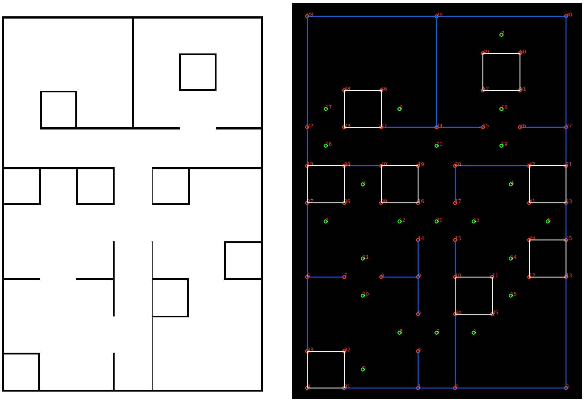
When the escape room challenge had taken place, and the first steps were taken for the hospital challenge, it was decided to make a test map. This way, our efforts could be tested in simulation. This test map had to encorporate a lot of possible scenarios, such as a corridor, multiple doors to one room, multiple cabinets in one room, and varyiong positions of cabinets within the rooms. This test map can be seen below. | |||
[[File:HospitalMap_cropped.png|center|600 px]] | |||
== Path Planning == | |||
Before the actual Path is planned a graph is generated of all possible paths in case there wouldn't be any obstructions (e.g. a closed door). | |||
To create a graph a minimal amount of checkpoints is wisely located on the map, visualized as the green dots in the [http://cstwiki.wtb.tue.nl/index.php?title=Embedded_Motion_Control_2019_Group_1#Test_map Test Map]. | |||
Once the graph is created and PICO has localised itself correctly the actual path planning can start. The graph for the hospital challenge is shown below | |||
[[File:GraphFinal.png|center|300 px]] | |||
For PICO's path planning a Dijkstra Algorithm is used. The algorithm returns the path with the least amount of checkpoints. Another important feature is that the path can be updated in case an obstruction is detected. In that case, PICO will choose a new path based on the least amount of checkpoints. Once PICO knows a certain checkpoint transition is unreachable this knowledge will be used for all future paths. | |||
== Localization == | |||
[[File:AD filter.png|thumb|upright=4|right|450px|Figure 1: Comparison extracting corners with/without AD-filter]] | |||
PICO's localization is built up from two main blocks; the extraction of corners using LRF data and using an unconstrained optimization problem. | |||
Firstly, the corner extraction. Initially for the escape room challenge a very simple local peak finder on the LRF data was used to extract corner points. Based on a local minimum/maximum it was determined whether it was a convex/concave corner. However, after the first challenge this method seemed not that sufficient. This is visualised in the upper part of Figure 1. | |||
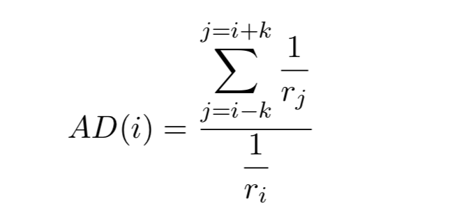
In the literature [https://www.semanticscholar.org/paper/High-Speed-Feature-Extraction-in-Sensor-Coordinates-Alempijevic/bfa559720741370ae3854e4af9363fbe14b2e918] a geometric approach is discussed in order to robustly detect corners (and extendable to features). For convenience the method is referred to as the 'AD-filter'. The AD-filter uses purely the range <math>r_i</math> at every index of the LRF data. The equation for the metric-value AD shows that it evaluates the range of indices left and right of the current index. If index <math>i</math> is located on a straight line without any corners in the vicinity of <math>k</math>-indices then AD(i)<math>\approx</math>0. However, when closing in on a corner at index <math>i</math> then at some point (i-k)< j <(i + k), and the trend of the range of the indices is not continuous. Therefore, AD(i) deviates from zero. If index <math>i</math> is exactly on a corner then the deviation from zero reaches a local minimum/maximum (see Figure 1). Minima smaller than zero represent concave corners, maxima greater than zero represent convex corners. Sequence of values approximately zero represent straight line segments. | |||
[[File:AD eq.png|center|frameless|upright=1]] | |||
In order to determine the minima and maxima of the AD-filtered data a highly modified version of the following peak-finder algorithm is used [https://github.com/claydergc/find-peaks]. It enables to set upper and lower bounds for convex and concave peaks in the AD-filtered data because real-life LRF data is very noisy. For example, the following additional features are built in to increase robustness and enhance selection of actual corners. A feature to detect corners at the end of line-segments. Another feature that clusters a set of corners to a single corner in the event of multiple corners within a certain Euclidean range (currently set to 0.1 [m]). As well as a feature that ignores corners that are placed at the end of the LRF array. | |||
The benefit of the proposed method for extracting corners ended up being very robust and very fast. The only downside is that in order to get it working properly quite a few parameters (five) have to be tuned in order to get a desirable result. Finally, the parameters have been tuned such that only corners with a high confidence rate are extracted. Because, extracting corners that in the real-world aren't actual corners will result in issues for the localization algorithm explained hereafter. | |||
[[File:PicovisualGroup1.gif|thumb|upright=8|right|Figure 2: PICO's visualization during execution]] | |||
A simulation of the Hospital map with PICO's visualization on shows how PICO navigates through the hospital and plotting the convex and concave corners that are detected. This is visualized in Figure 2. The code used for the corner detection can be reviewed in this [https://gitlab.tue.nl/EMC2019/group1/snippets/158 code snippet]. | |||
As mentioned before, for the localization of PICO an uncontrained optimization problem is solved. This is done with a L-BFGS algorithm, the optimization toolbox dlib [http://dlib.net/] is used to minimize an objective function. The localization problem is a combination of odometry data, previous localized position and worldmodel perception (the extracted corners defined earlier). | |||
First, at the starting pose of PICO a global origin is placed. As soon as PICO starts to drive in any direction the odometry data is used to estimate a new position. PICO's perception of the environment changes, the percepted corners are plotted on a global scale using the algorithms initial value. The initial value for the algorithm is a combination of the last-known location and the odometry data. The problem is solved for a vector x = [dx dy d<math>\theta</math>]' which corresponds to the required x,y,<math>\theta</math> in order to get from the global origin to PICO's location. | |||
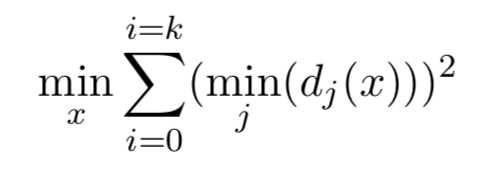
For an m-amount of percepted corners the distance to an n-amount of total corners on the 'known' map are calculated. Resulting in an mxn-matrix, taking the minimum value of every row gives the distance between a percepted corner and it's closed pairing corner on the real map. Summing the quadratic minimum distance of all percepted corners results in the objective function ([https://gitlab.tue.nl/EMC2019/group1/snippets/156 code snippet]). By using the L-BFGS the quadratic minimum distance of all percepted corners are minimised such that a local minima is reached ([https://gitlab.tue.nl/EMC2019/group1/snippets/157 code snippet]). By reaching a minima a solution is found for <math>x</math>. However, the objective function is not convex, therefore there are multiple local minima that can be acquired. | |||
[[File:cost function.png|center|frameless|upright=1]] | |||
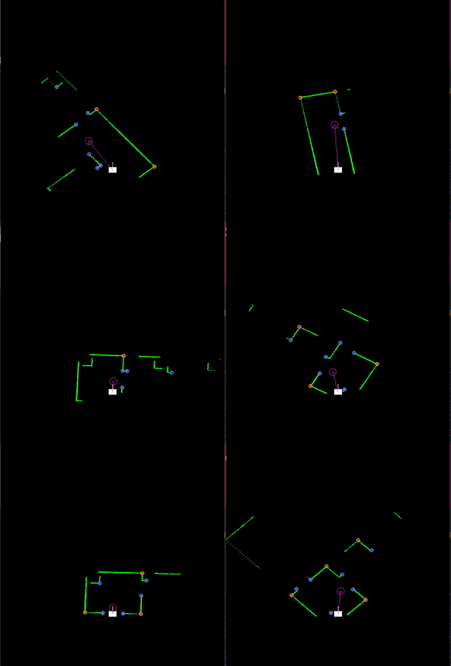
In order to deal with multiple local minima the localization is to be executed every timestep (algorithm is solved in approx. 3 ms) such that based on the amount of percepted corners a maximum threshold is set that throws away a solution if the objective function value is above the threshold. In Figure 3 is shown with multiple coordinate systems how the algorithm works. | |||
[[File:Localization matlab.png|thumb|upright=4|center|800px|Figure 3: Visualization of localization procedure]] | |||
== Obstacle Avoidance == | |||
Because the hospital map contains both static and dynamic obstacles, an obstacle avoidance controller is designed. This controller prevents PICO from bumping into the obstacles by performing different tasksets depending on the nature of the obstacle. The controller is initialized when PICO detects an obstacle when it is rotated to or driving towards the next checkpoint of its trajectory. In the event that PICO detects an obstacle when rotated towards its checkpoint, monitor 2 causes PICO to switch to state 6, which lets PICO drive up against the obstacle. Then, it goes in idle mode for 5 seconds to determine whether the obstacle is of static or dynamic nature. | |||
[[File:StaticObstacleAvoidance_group1.gif|frame|right|Static obstacle avoidance]] | |||
If the obstacle has not moved after 5 seconds, the average of the data front left of PICO is compared to the average of the data front right of PICO. Afterwards, PICO moves to the side of which the average is the highest, indicating the most space as the sensor can see the furthest and thus the highest chance of avoiding the obstacle. PICO then keeps driving sideways until it has passed the obstacle with a margin, or drives the opposite way in the event that PICO cannot pass the obstacle on the side with the highest average. If the latter occurs, PICO tries to pass the obstacle on the other side plus margin. If it still cannot pass the obstacle then, monitor 8 enables PICO to delete the checkpoint and a new route is planned. If PICO is able to drive sideways until the obstacle is out of its front sight and the extra margin is driven to ensure that PICO can pass the obstacle safely, it moves forward and checks the data on its left and right side to determine when it has passed the obstacle plus margin. This is monitored by monitor 9, which enables PICO to orient towards the checkpoint once more in the hope that the path towards the checkpoint is now clear. A visualization of the static obstacle avoidance is given on the right. | |||
If the obstacle moves within the 5 seconds in which PICO is idle, high alert mode is enabled. This mode causes PICO to define a safe zone of half a circle with a radius of 40 cm around itself. PICO then remains idle for another five seconds to check whether this obstacle is actually dynamic or that it is caused by sensor noise. If the safe zone became free within the five seconds that PICO was idle, it can be concluded that the obstacle was dynamic as PICO was not moving, so the obstacle was. It then drives forward at a low speed while closely monitoring its safe zone until it encounters another obstacle or is 0.2 metres within the next checkpoint. It is also possible that PICO encounters a static obstacle when in high alert mode. For this reason, a failsafe is implemented by monitors 8 and 10 which enable PICO to switch to a state that makes PICO move in the opposite direction of the obstacle in the event that the obstacle has remain static for 5 seconds. | |||
== UML generation == | |||
For the UML generation additional software is required, java, Graphviz and plantuml.exe. After installing these programs a text file has to be created with PlantUML commands, like this example called | |||
''testUML.txt'': | |||
@startuml | |||
title Message/Job Queue + Workers State Chart | |||
state "Idle Queue" as Idle <br> | |||
[*] -> Idle<br> | |||
Idle -> Queue : Task Arrives<br> | |||
Queue : Task placed in queue.<br> | |||
Queue -> Worker : Worker collects Task<br> | |||
Worker -> ProcessingTask | |||
state ProcessingTask { <br> | |||
[*] --> long1 <br> | |||
long1 --> ProcessData : Enough Data <br> | |||
} | |||
ProcessingTask -> [*] | |||
@enduml | |||
The creation of the text file is automated by a function in the code. After running the code created text file appears in the bin folder. | |||
Then, run PlantUML, using "testUML.txt" as input. The output is an image which is written to an image file on disk. For example: | |||
java -jar plantuml.jar "testUML.txt" | |||
If you type this in your command window while being in the folder where both the text file as the plantuml executable are located this results in a file called testUML.png and is shown below. | |||
[[File:Test.png|thumb|upright=4|center|600px|Example stateflow created with plantuml]] | |||
== Simulation Hospital challenge == | |||
A simulation of the hospital challenge at double speed is shown below. PICO needs to visit cabinets 3, 2 and 0. It looks at its Graph to plan a route through checkpoints to the first cabinet. Everything works just fine for the first cabinet. This is done for the second cabinet as well, but upon arriving at a closed door, it stops. PICO recognizes that it cannot continue with its plan, and plans another route through the corridor by deleting a connection of the Graph and again calculating the shortest path. Furthermore, to know where PICO is, it constantly looks at all the corners it percepts with its laser range finder and fits them on its map (see the section Localization). This way, PICO is able to autonomously navigate through the hospital. | |||
[[File:HospitalSimGroup1.gif|frame|center|upright=0.7|Hospital challenge simulation at double speed]] | |||
== Testing prior to the Hospital challenge == | |||
Since the hospital map was known a priori, during the last week of testing on PICO the hospital map was built on the robocup field. During the testing hours, PICO was able to complete a simplified challenge, as there were no obstacles present on its route. The route used can be seen below. | |||
[[File:FinalMap_FinalMap_withFeatures_Crop.png|frame|center|The hospital map with checkpoints.]] | |||
PICO is assigned to visit cabinets 2 and 1. PICO initially orients itself, making sure it knows where it is. PICO now calculates a route towards cabinet 2. If the route is calculated, PICO rotates towards the first checkpoint (15), moves through the door towards checkpoint 16, and turns towards checkpoint 10. | |||
[[File:simplifiedHospital2.gif|frame|center|PICO's simplified hospital challenge]] | |||
PICO drives towards checkpoint 10, and drives through the second door towards checkpoint 8. It corrects itself once it comes too close to the doorpost, and rotates and moves towards checkpoint 3. Checkpoint 3 was introduced to make sure PICO does not drive into cabinet 2 when it comes from checkpoint 8. | |||
PICO rotates towards checkpoint 0, which is the checkpoint at the first cabinet. As can be seen, its margins are a bit off, but when it reaches the cabinet, it plans a new route towards cabinet 1, and once the route is planned, it rotates towards the next checkpoint (3), and drives towards it. | |||
PICO drives through the door, again correcting itself when it comes too close to the doorpost, towards checkpoint 4, 5, 6, and 7 which are all in a straight line, so it does not need to rotate. Then, it rotates towards checkpoint 2, which is the checkpoint at the second cabinet. When PICO reaches the final cabinet, it turns off. | |||
== Results Hospital challenge == | |||
The hospital challenge was the final test for PICO and us to check whether the software could handle the imperfections of the real world. In the simulation, PICO is able to succesfully visit cabinets on the given map in any arbitrary order. It was also able to avoid obstacles and re-plan its route when e.g. a door was closed. | |||
During the first try of the Hospital Challenge PICO oriented itself, planned its route towards the first cabinet and drove towards the door of the first room, into the hallway. | |||
[[File:HospitalChallenge_group10.gif|frame|center|PICO's first try at the hospital challenge]] | |||
PICO did not care about the dynamic obstacle, since it was not in its direct path, and therefore kept going towards its next checkpoint, at the corner of the corridor. | |||
Then, PICO drove past the obstacle with a slightly smaller margin than expected, but still avoiding collision with the obstacle. | |||
As can be seen, PICO then does not turn towards the door when it passes by it. It moves towards the wall, since its localization is not correct and therefore it does not know where it is. When PICO arrives at the wall, it turns 180 degrees and moves backwards towards the corridor, trying to localize again. Unfortunately this is not done correctly, and therefore PICO drives into a wall. | |||
After try 1, at our request, the obstacle was removed from the corridor. This would have made the localization for PICO much more likely to succeed, as it did as such in the simulations. When starting PICO again, we did not hit 'pstart' again. This resulted in the odometry data not being reset, and therefore resulting in the orient controller not working correctly. As can be seen below, PICO did not localize correctly, and drove towards the 1st cabinet instead of its route towards cabinet 0. | |||
[[File:HospitalChallenge2-gif.gif|frame|center|PICO's second try at the hospital challenge]] | |||
== | = Learning points = | ||
The following points have been valuable lessons in this project:. | |||
#Although the software architecture is very intuitive to use and of a modular nature, it is quite prone to user errors. As every event and state requires an ID, this becomes cumbersome as the complexity of the plan increases. In the future, it is much wiser to let the software number the components in the order that they are entered. To connect states together, unique strings could be used. | |||
#The plan state machine has grown to be rather complex. Although this does not introduce any complexity in the code, because of the modular design of the software architecture, it is hard to keep an overview even in the conceptual schematic. Instead of introducing a new state for every piece of functionality, one can use a few if statements in function bodies of states. This has to be done with care, as having simple function bodies is one of the key selling points of this software architecture, but keeping the number of states low is advantageous. | |||
#It might have been worth it to use a slightly more complex method to move from checkpoint to checkpoint. Merely checking whether the checkpoint is within a certain distance can lead PICO to miss checkpoints from time to time, requiring it to rotate all the way back and drive towards the checkpoint again. Essentially, we loved simple solutions for most problems but in this case we could have been more careful not to oversimplify it. | |||
#As the software architecture is an important part of the project, it is recommended in the future to have multiple people involved in its design. This makes it easier to implement structural improvements. | |||
= Code snippets = | |||
[https://gitlab.tue.nl/EMC2019/group1/snippets/143 Main event loop] | |||
[https://gitlab.tue.nl/EMC2019/group1/snippets/158 Corner Detection] | |||
[https://gitlab.tue.nl/EMC2019/group1/snippets/157 Localization] | |||
[https://gitlab.tue.nl/EMC2019/group1/snippets/156 Objective function] | |||
Latest revision as of 23:28, 21 June 2019
Group members
1. Toos van Gool - 0885992
2. Paul Janssen - 1273507
3. Jochem Manders - 0858988
4. Max van Meer - 0951669
5. Raoul Surie - 0810262
Design Document
An initial design report was created to assist in the design of the software, which can be found here: Initial Design Report Group 1. The parts from the report can also be found here on this wiki.
Introduction
The information structure proposed in this document is used to design the software of an autonomous robot, named PICO. PICO has to complete an escape room challenge and a hospital room challenge. To ensure good performance in these challenges, the requirements and specifications are defined initially. Afterwards, the hardware and software components are identified and the functions of the software components are defined. Finally, the interfaces between the components and functions are explained.
Requirements
| Requirements | Specifications |
|---|---|
| PICO should execute all tasks autonomously. | Once PICO is started, no interaction is allowed. |
| PICO should perform all tasks without bumping into a wall. | The forward distance of PICO with respect to an object should always be at least 15 cm, sideways contact is not allowed. |
| Minimize oscilation of PICO to ensure correct sensor data. | PICO’s acceleration profile should be smooth. |
| PICO cannot exceed speed limitations. | PICO’s maximum translational velocity is 0.5 m/s. |
| PICO’s maximum rotational velocity is 1.2 rad/s. | |
| PICO should be aware of its surroundings. | PICO should create and update a (local) map of its surroundings. |
| PICO should minimize its stationary time. | PICO should not stand still for longer than 30 seconds. |
| PICO should terminate when the objective is reached. | ERC: PICO should stop when its rear wheels have crossed the finish line. |
| PICO should fulfill its objective as fast as possible. | ERC: PICO should exit the room within 5 minutes. |
Components
Hardware
The hardware of PICO consists of the following components:
- Sensors: Laser Range Finder (LRF), and wheel encoders (odometry)
- Actuators: Holonomic base (omni-wheels)
- Computer: Intel i7 running Ubuntu 16.04
Information
The information architecture of PICO consists of the following components
- World model
- Perceptor
- Planner
- Controller
- Monitor
The world model contains the state of all activities on which the other components base their actions. The perceptor functions as a data processor that creates a perception of the world around PICO by interpreting the sensor data. The planner contains a state machine in which the strategy of a process is implemented and plans actions based on this state machine. The controller ensures that PICO executes tasks in a correct manner and the monitor ensures that problematic situations, such as encountering static or dynamic obstacles, are resolved. The manner in which these components communicate among each other is described in the Section on Interfaces.
Functions
| Function | Description |
|---|---|
| Controller | |
| OrientInRoom | Determines whether towards move to an exit or a wall. |
| DriveToWall | Drives PICO towards a predefined wall. |
| DriveAlongWall | Drives PICO within a certain distance along a wall. |
| MoveToExit | Drives to a point allocated in front of an exit. |
| MoveThroughCorridor | Manoeuvers PICO through the middle of a corridor. |
| AvoidStationaryObstacle | Adjusts trajectory to avoid stationary obstacle. |
| AvoidDynamicObstacle | Adjusts trajectory to avoid dynamic obstacle. |
| TerminateActivity | Shuts down PICO when objective is reached. |
| MoveToTrajectory | Determines a feedforward trajectory to end up at desired trajectory. |
| Monitor | |
| FindProximityToWall | Updates world model state to avoid objects. |
| FindConcaveCorner | Adds new concave corner to the world model. |
| FindConvexCorner | Adds new convex corner to the world model. |
| TrackTrajectory | Updates world model that actual trajectory deviates too much from desired trajectory. |
| FindStationaryObstacle | Updates world model with new stationary obstacle. |
| FindMovingObstacle | Updates world model with new dynamic obstacle. |
| FindExit | Updates world model state when two concave corners are found in close proximity. |
| FindCorridor | Upadtes world model state when an exit with extending walls is found in close proximity. |
| FindCabinet | Updates world model if cabinet is found. |
| LostExit | Updates world model state if an exit is lost when moving towards one. |
| LostWall | Updates world model state if a wall is lost when tracking one. |
Specifications
A couple of important specifications of PICO are:
- The maximum speed of the robot is limited to ±0.5 m/s translationwise and ±1.2 rad/s rotationwise.
- PICO is 41 cm wide and 35 cm deep.
- The LaserRangeFinder has a maximum measurable distance of 10 m and a scope of ±2 rad, which is divided into 1000 equal parts.
Interfaces
The interfaces between the different components is illustrated below.
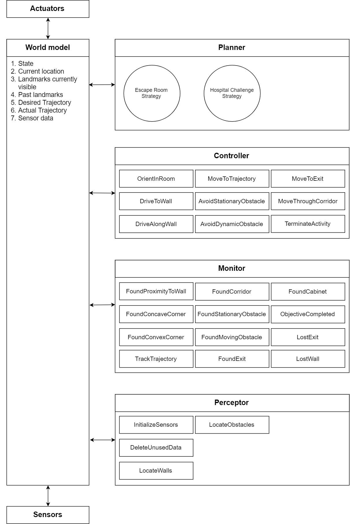
All components communicate with the world model to ensure that they operate using the same perception of surroundings and from the same tasks. This is realized by allowing the components to perform certain tasks based on the state of the world model. For example, if the planner notices that the exit is found in the escape room challenge, the state is changed to ExitRoom. The change of this state causes the controller, monitor and perceptor to only use the functions relevant to leaving the room. In this case, the functions of the controller could be MoveToExit,MoveToTrajectory and AvoidStationaryObstacle.
The world model thus contains the state on which the components base their events, current location with respect to a certain reference (e.g. the wall besides PICO or the position within a room), landmarks currently visible and past landmarks to determine the trajectory, a desired and actual trajectory and the incoming sensor data.
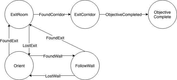
The planner contains both strategies for the challenges. The strategy to be used in the escaperoom challenge is illustrated below. PICO starts in the Orient state to immediately find the exit if the exit is in sight, and otherwise a wall to follow. If a wall is found, the monitor indicates this by updating the world model. The planner notices this event and sets the state of the world model to FollowWall. This process continues until the state ObjectiveComplete is reached.
Software Architecture
The information architecture shown in the Initial Design Document is made to a modular software architecture, which can be used for both the Escape Room Challenge and the Hospital Challenge. In this section, this software architecture will be elaborated.
Summary
A modular software architecture was created in which the event loop always remains the same. A plan is seen as a state machine of controllers, which are in turn state machines. These state machines can be constructed in a user friendly manner, using function pointers to prevent code duplication and to keep a clear overview of the robot's strategy. Monitors can be created in an equally modular way. Additionally, all relevant information passes through a central WorldModel. Monitors and controllers that are not relevant to the current state of the Plan state machine are not executed to spare resources. Adding semantic information such as Corners or Checkpoints to the WorldModel is easy and scalable.
User manual
To let the robot do anything, whether it is escaping a room or navigating through a hospital, the following steps should be taken.
Creating the concept
- Draw the plan on paper as a state machine. Give all states an ID (int), starting from zero. Give all connections (events) an ID as well, starting from zero.
- Every state of the plan corresponds to a controller. Draw each controller on paper as a state machine. Again give an ID (int) to each state. Note that the numbering is shared by all controllers, but that it is separate from the plan. For example, the plan can have states with IDs 0, 1, 2. These three controllers could have states with IDs (0, 1, 2, 3), (4, 5), (6, 7, 8). The same numbering rule holds for connections (events).
- Every connection (event) of the plan corresponds to a monitor. Write down in pseudo-code what exactly this monitor needs to see from the WorldModel before it triggers an event.
Programming the plan, controllers and monitors
- Label all the state IDs and connection IDs as macros (all caps) in config.h.
- Create the plan in plan.cpp. To do this, create a function such as StateMachine getEscapeRoomPlan() that is called by main.cpp. The plan is created as follows.
- Initialize a StateMachine object plan with the initial state ID, the amount of states and the amount of connections.
- For every state, create a State object with its state ID. Add this State object to the StateMachine object.
- For every connection, create a Connection objects with its connection ID, the state ID from which this arrow points, and the state ID to which this arrow points. Add these Connection objects to the StateMachine object.
- Create the controllers in controllers.cpp. Write a function such as ControllerCollection getTestControllers(emc::IO *io, WorldModel *wm). Then create the controllers as follows.
- Initialize an std::Vector<StateMachine> controllers;.
- In the same order as the definition of the state IDs, for each controller, create a StateMachine object with its initial state ID, the amount of states and the amount of connections.
- For each state in every controller, create a State object. Pass to the constructor the state ID. In addition, pass the name of a void(emc::IO*) function that you write in the same source file. This is the body that will be executed in every iteration of the event loop. For example, if the active state is 'driveBackwards', then the function body could be io->sendBaseReference(-1*MAX_FORWARD_SPEED,0,0);. Lastly, pass to the constructor a pointer to an emc::IO object. Add each State object to its corresponding StateMachine object and add each StateMachine object to the vector controllers.
- When all StateMachine objects are made, return a ControllerCollection object made from the vector of Statemachine objects, the ID of the initial controller to be active and the pointer to the WorldModel object.
- Create the monitors in monitors.cpp. Write a function MonitorCollection getEscapeRoomControllerMonitors(WorldModel *worldModel). Then fill it in as follows. Note that the monitors for the plan are created in a separate (but similar) function as the monitors for the controllers.
- Initialize an std::vector<Monitor> monitors; and an std::vector<int> activeIds;. These will contain the monitors for the controllers and the IDs of all active controller monitors.
- Create each monitor by passing to the constructor of the Monitor class a pointer to the WorldModel, the ID of the monitor and the name of the monitor function. The monitor function is defined in the same source file and is of the form void mymonitor(WorldModel *wm). This function should look at the WorldModel and execute wm->addControllerEvent(monitorID) (or addPlanEvent for plan monitors). Then add the Monitor object to the vector of monitors and fill the vector of initial active monitor IDs.
- Return a MonitorCollection of the Monitor objects and the initial active monitor IDs.
- Repeat the above steps for the plan monitors in a separate function.
- Integrate everything in main.cpp by simply editing the function names to the ones that you just created. The event loop does not have to be edited because of the modular design.
Selling points of the software architecture
- The modular software structure enables a developer to test and validate software independently.
- A full plan with corresponding state machines can be implemented in the sofware architecture in an intuitive manner.
- Controllers and monitors can be reused indefinitely.
- Only controllers and monitors relevant to the current state are executed to spare resources.
- No grids or potential fields are used for path planning or route execution.
- The software modules only communicate through a world model and not among each other to add context to data.
- Information is interpreted semantically where possible. New information can be interpreted semantically in the world model in a easy and scalable method.
- The architecture outputs a UML diagram of the implemented state machines to check if they are implemented correctly, and to troubleshoot if necessary.
Technical overview
The software architecture consists of a WorldModel object, a Perception object, a StateMachine object for the plan, a ControllerCollection object and a MonitorCollection object. Each of these components will be discussed below, starting with the main program. The simplified overview of the software architecture shown on the right is used as aid to describe the components.
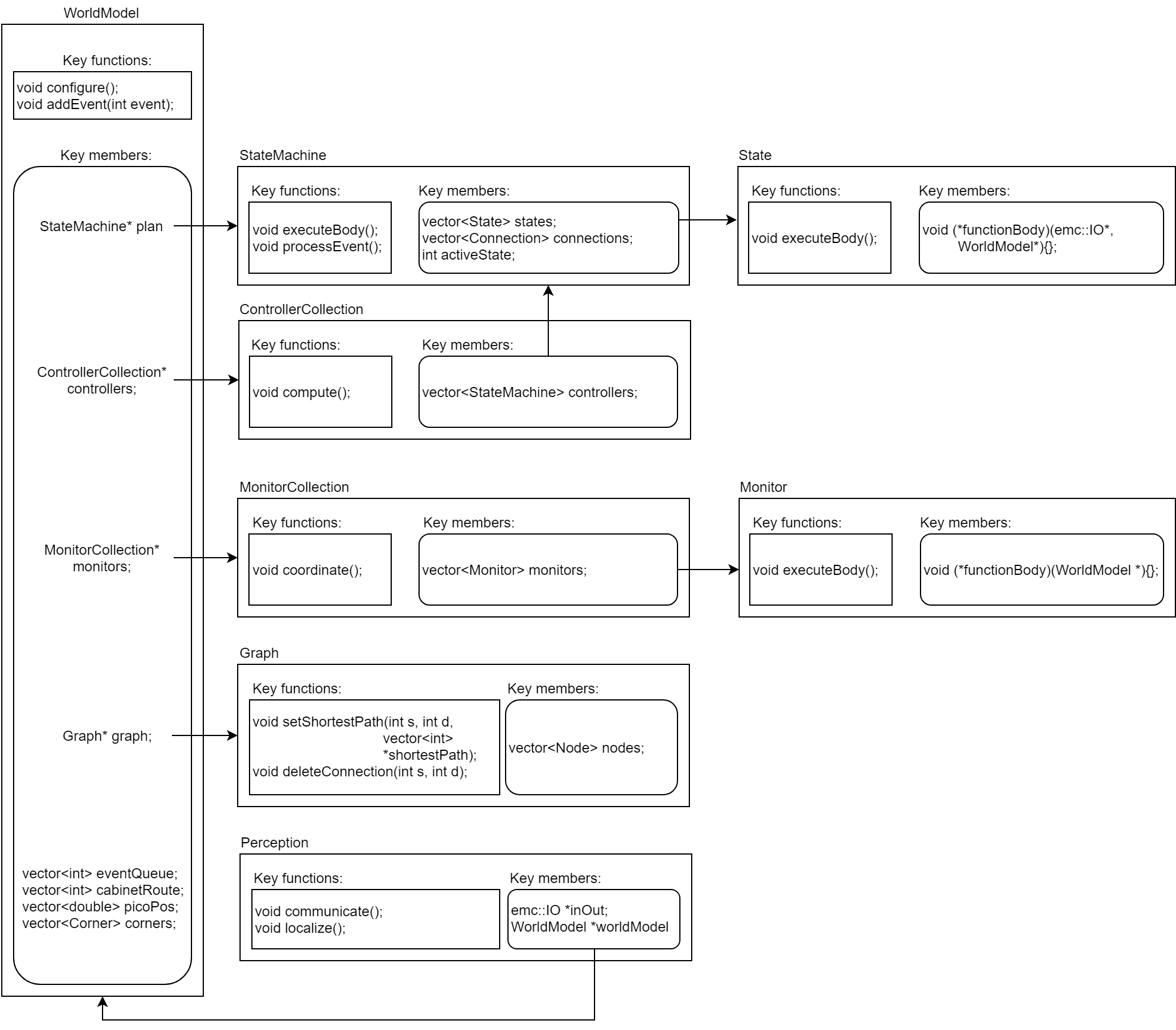
- Main program: event loop. The event loop is shown in a code snippet in Gitlab. Everything is clearly separated and there is a clear overview of which class is doing which tasks. The controllers and monitors are loaded from a separate file, that also includes all monitor and controller functions. See the user manual above for more information.
- WorldModel: This component is what brings everything together. The configure() function processes the event queue that was filled by the monitors, and switches active controllers and monitors accordingly.
- Plan (StateMachine with State objects). A StateMachine object, such as the plan, contains several State objects and Connection objects that describe their relations. Each State contains a function pointer which is execution upon calling the executeBody() function. This executeBody() function can be configured to invoke either one of the controllers (which are StateMachine objects), or a function pointer supplied by the user.
- Controllers: as seen in the overview, the controllers are put in a ControllerCollection object, which contains a vector of StateMachine objects and a function compute() to invoke the function body of only the active controllers.
- Monitors: these work similar to the controllers, as can be seen in the overview. The function bodies that are passed to Monitor Objects have to invoke worldModel->addEvent(int event), when a certain condition is met.
- Graph: the functionality of the graph is explained in more detail elsewhere. Simply put, the functions displayed in the overview show how nodes (checkpoints) can be used and where a shortest path can be generated.
- Perception: this object is the only instance which is reading the laser data and odometry information. It includes the localization functionality and updates the position of PICO in the WorldModel. In addition, the OpenCV window is managed in this class.
The Escape Room Challenge
The simulation
For the first challenge, we built a wall-follower combined with an exit detector. As can be seen in the simulation gif, PICO follows the wall with lazy control: PICO corrects itself only in the event that it comes too close to a wall. If PICO almost is at a wall, it rotates 90 degrees to the right, and follows the next wall. If it finds an exit, it turns left, and follows the corridor towards the finish line.
Result of the Escape Room challenge
As can be seen in the gif below, during the first attempt PICO drove into the wall immediately. This has to do with the margins we set on PICO to avoid the walls, which were not set around PICO but only in front of it. Therefore, the margin was not large enough, and it drove into a wall.
PICO was repositioned, and another try was given. During the second run, PICO drove towards the wall, and turned right when it was 0.3 meters in front of it. It then followed the wall on its left, until it found another wall in front of it. Then it turned right again, to follow the wall on its left. Due to a slight gap in the wall PICO thought it had found the exit, and turned towards it. Since this was not the actual exit, the challenge failed.
Learning points Escape Room challenge
The outcome of the Escape Room Challenge itself is that the plan was not robust enough. The small gap in the wall made PICO think that the exit was found already, resulting in a collision with a wall and failing the Escape Room Challenge. The overall learning points that can be taken from this are:
- The margins set on PICO should be set a bit larger, since as can be seen in the second .gif above, PICO almost bumped into one of the walls and made the 'referee' shut it down.
- When defining a distance w.r.t. a wall / object, an average of a couple of data points should be taken (so a cone of points) instead of a single datapoint. This to make sure PICO will be able to cope with the real world which is never perfect.
The Hospital Challenge
Strategy
For the hospital challenge, a strategy is established consisting of 6 controllers: Orient, RoutePlanned, ExecuteRoute, CheckpointAvailability, ObstacleAvoidance and Terminate. Combining these controllers enables PICO to autonomously execute a route in which an arbitrary number of cabinets is visited. These controllers also enable PICO to function correctly for the map and its variations due to static and dynamic obstacles, and deviations in the provided map versus the real world. To convey a clear image of the hospital challenge strategy, it is illustrated in the figure at the end of this section.
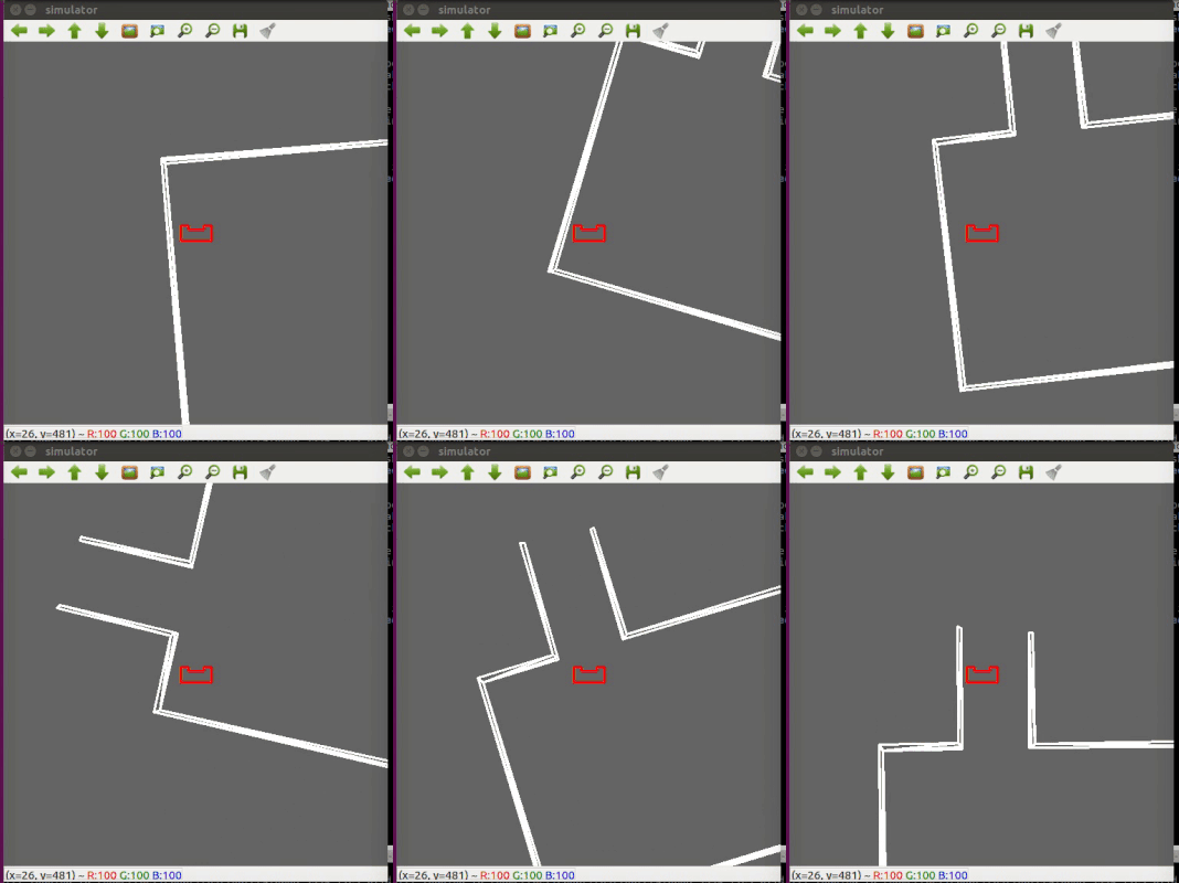
At the start of every attempt of the hospital challenge, PICO starts in the Orient state. This state functions as a calibration for PICO to position itself in the most favorable position for the localization, which is the position in which PICO is looking into the room and not to a wall or a corner. The Orient controller thus heavily depends on the conditions of the starting area of PICO in the hospital challenge. This area is given prior to the challenge and consists of an area of one square meter in which PICO can be placed arbitrarily. For this reason, four possibilities are considered: the square meter lies in the middle of a room (against no wall), against a wall, in a corner (and thus against two walls), or against three walls. In the event that the starting position does not lie against a wall, the Orient controller is redundant and thus eliminated from the strategy. For the simulations, an assumption is made that PICO will start in a corner, so the Orient controller is implemented for this case. This controller is illustrated on the right. Note that PICO starts in the correct orientation to localize in the simulation. This is, however, not a certainty in the actual challenge. For the other two possibilities, only a state machine has been established. Fortunately, the starting area of PICO for the final challenge indeed lay in a corner, meaning that no other Orient controller had to be implemented.
Once PICO is oriented, PICO switches to the Localize controller. The exact algorithm applied by PICO to localize is explained in the section 'Localization'. When PICO has localized itself, it plans a route based on its current position, the position of the cabinet it has to visit next, and all the checkpoints in between. The checkpoints are visualized as the green dots in the Test Map. In case multiple routes are possible, e.g. due to the fact that a room has multiple doors through which PICO can enter, PICO picks the route with the least amount of checkpoints.
Once PICO is localized and its route is planned, its state switches to the ExecuteRoute state. In this state, PICO will follow the route it has planned along the cabinets.
The ExecuteRoute controller starts with PICO rotating left, until the checkpoint it needs to visit next is in its front line of sight. Then, if PICO does not see any obstruction in between itself and the next checkpoint, it simply moves towards it. If PICO notices obstruction between itself and the checkpoint, it switches to the ObstacleAvoidance controller. The manner in which PICO avoids static and dynamic obstacles is explained in the section 'Obstacle Avoidance'. For now, assume that PICO is able to move to every checkpoint without any obstacles.
If the checkpoint reached is not the final checkpoint, PICO again starts rotating left, until the checkpoint it needs to visit is in its front line of sight. If the checkpoint reached is the final checkpoint, it has reached a cabinet, and thus has to position itself in the area in front of the cabinet by rotating towards the cabinet. If PICO is correctly positioned in front of the cabinet, it makes a sound signal to indicate that it has reached the cabinet.
If the cabinet reached is not the final cabinet, PICO switches to the Localize controller again, to localize again, and plan its route towards the next cabinet. When PICO has reached the final cabinet, it gives a final sound signal, indicating that it has succesfully carried out its assignment.
Test map
When the escape room challenge had taken place, and the first steps were taken for the hospital challenge, it was decided to make a test map. This way, our efforts could be tested in simulation. This test map had to encorporate a lot of possible scenarios, such as a corridor, multiple doors to one room, multiple cabinets in one room, and varyiong positions of cabinets within the rooms. This test map can be seen below.
Path Planning
Before the actual Path is planned a graph is generated of all possible paths in case there wouldn't be any obstructions (e.g. a closed door). To create a graph a minimal amount of checkpoints is wisely located on the map, visualized as the green dots in the Test Map. Once the graph is created and PICO has localised itself correctly the actual path planning can start. The graph for the hospital challenge is shown below

For PICO's path planning a Dijkstra Algorithm is used. The algorithm returns the path with the least amount of checkpoints. Another important feature is that the path can be updated in case an obstruction is detected. In that case, PICO will choose a new path based on the least amount of checkpoints. Once PICO knows a certain checkpoint transition is unreachable this knowledge will be used for all future paths.
Localization

PICO's localization is built up from two main blocks; the extraction of corners using LRF data and using an unconstrained optimization problem.
Firstly, the corner extraction. Initially for the escape room challenge a very simple local peak finder on the LRF data was used to extract corner points. Based on a local minimum/maximum it was determined whether it was a convex/concave corner. However, after the first challenge this method seemed not that sufficient. This is visualised in the upper part of Figure 1.
In the literature [1] a geometric approach is discussed in order to robustly detect corners (and extendable to features). For convenience the method is referred to as the 'AD-filter'. The AD-filter uses purely the range [math]\displaystyle{ r_i }[/math] at every index of the LRF data. The equation for the metric-value AD shows that it evaluates the range of indices left and right of the current index. If index [math]\displaystyle{ i }[/math] is located on a straight line without any corners in the vicinity of [math]\displaystyle{ k }[/math]-indices then AD(i)[math]\displaystyle{ \approx }[/math]0. However, when closing in on a corner at index [math]\displaystyle{ i }[/math] then at some point (i-k)< j <(i + k), and the trend of the range of the indices is not continuous. Therefore, AD(i) deviates from zero. If index [math]\displaystyle{ i }[/math] is exactly on a corner then the deviation from zero reaches a local minimum/maximum (see Figure 1). Minima smaller than zero represent concave corners, maxima greater than zero represent convex corners. Sequence of values approximately zero represent straight line segments.
In order to determine the minima and maxima of the AD-filtered data a highly modified version of the following peak-finder algorithm is used [2]. It enables to set upper and lower bounds for convex and concave peaks in the AD-filtered data because real-life LRF data is very noisy. For example, the following additional features are built in to increase robustness and enhance selection of actual corners. A feature to detect corners at the end of line-segments. Another feature that clusters a set of corners to a single corner in the event of multiple corners within a certain Euclidean range (currently set to 0.1 [m]). As well as a feature that ignores corners that are placed at the end of the LRF array.
The benefit of the proposed method for extracting corners ended up being very robust and very fast. The only downside is that in order to get it working properly quite a few parameters (five) have to be tuned in order to get a desirable result. Finally, the parameters have been tuned such that only corners with a high confidence rate are extracted. Because, extracting corners that in the real-world aren't actual corners will result in issues for the localization algorithm explained hereafter.
A simulation of the Hospital map with PICO's visualization on shows how PICO navigates through the hospital and plotting the convex and concave corners that are detected. This is visualized in Figure 2. The code used for the corner detection can be reviewed in this code snippet.
As mentioned before, for the localization of PICO an uncontrained optimization problem is solved. This is done with a L-BFGS algorithm, the optimization toolbox dlib [3] is used to minimize an objective function. The localization problem is a combination of odometry data, previous localized position and worldmodel perception (the extracted corners defined earlier).
First, at the starting pose of PICO a global origin is placed. As soon as PICO starts to drive in any direction the odometry data is used to estimate a new position. PICO's perception of the environment changes, the percepted corners are plotted on a global scale using the algorithms initial value. The initial value for the algorithm is a combination of the last-known location and the odometry data. The problem is solved for a vector x = [dx dy d[math]\displaystyle{ \theta }[/math]]' which corresponds to the required x,y,[math]\displaystyle{ \theta }[/math] in order to get from the global origin to PICO's location.
For an m-amount of percepted corners the distance to an n-amount of total corners on the 'known' map are calculated. Resulting in an mxn-matrix, taking the minimum value of every row gives the distance between a percepted corner and it's closed pairing corner on the real map. Summing the quadratic minimum distance of all percepted corners results in the objective function (code snippet). By using the L-BFGS the quadratic minimum distance of all percepted corners are minimised such that a local minima is reached (code snippet). By reaching a minima a solution is found for [math]\displaystyle{ x }[/math]. However, the objective function is not convex, therefore there are multiple local minima that can be acquired.
In order to deal with multiple local minima the localization is to be executed every timestep (algorithm is solved in approx. 3 ms) such that based on the amount of percepted corners a maximum threshold is set that throws away a solution if the objective function value is above the threshold. In Figure 3 is shown with multiple coordinate systems how the algorithm works.

Obstacle Avoidance
Because the hospital map contains both static and dynamic obstacles, an obstacle avoidance controller is designed. This controller prevents PICO from bumping into the obstacles by performing different tasksets depending on the nature of the obstacle. The controller is initialized when PICO detects an obstacle when it is rotated to or driving towards the next checkpoint of its trajectory. In the event that PICO detects an obstacle when rotated towards its checkpoint, monitor 2 causes PICO to switch to state 6, which lets PICO drive up against the obstacle. Then, it goes in idle mode for 5 seconds to determine whether the obstacle is of static or dynamic nature.
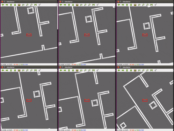
If the obstacle has not moved after 5 seconds, the average of the data front left of PICO is compared to the average of the data front right of PICO. Afterwards, PICO moves to the side of which the average is the highest, indicating the most space as the sensor can see the furthest and thus the highest chance of avoiding the obstacle. PICO then keeps driving sideways until it has passed the obstacle with a margin, or drives the opposite way in the event that PICO cannot pass the obstacle on the side with the highest average. If the latter occurs, PICO tries to pass the obstacle on the other side plus margin. If it still cannot pass the obstacle then, monitor 8 enables PICO to delete the checkpoint and a new route is planned. If PICO is able to drive sideways until the obstacle is out of its front sight and the extra margin is driven to ensure that PICO can pass the obstacle safely, it moves forward and checks the data on its left and right side to determine when it has passed the obstacle plus margin. This is monitored by monitor 9, which enables PICO to orient towards the checkpoint once more in the hope that the path towards the checkpoint is now clear. A visualization of the static obstacle avoidance is given on the right.
If the obstacle moves within the 5 seconds in which PICO is idle, high alert mode is enabled. This mode causes PICO to define a safe zone of half a circle with a radius of 40 cm around itself. PICO then remains idle for another five seconds to check whether this obstacle is actually dynamic or that it is caused by sensor noise. If the safe zone became free within the five seconds that PICO was idle, it can be concluded that the obstacle was dynamic as PICO was not moving, so the obstacle was. It then drives forward at a low speed while closely monitoring its safe zone until it encounters another obstacle or is 0.2 metres within the next checkpoint. It is also possible that PICO encounters a static obstacle when in high alert mode. For this reason, a failsafe is implemented by monitors 8 and 10 which enable PICO to switch to a state that makes PICO move in the opposite direction of the obstacle in the event that the obstacle has remain static for 5 seconds.
UML generation
For the UML generation additional software is required, java, Graphviz and plantuml.exe. After installing these programs a text file has to be created with PlantUML commands, like this example called
testUML.txt:
@startuml
title Message/Job Queue + Workers State Chart
state "Idle Queue" as Idle
[*] -> Idle
Idle -> Queue : Task Arrives
Queue : Task placed in queue.
Queue -> Worker : Worker collects Task
Worker -> ProcessingTask
state ProcessingTask {
[*] --> long1
long1 --> ProcessData : Enough Data
}
ProcessingTask -> [*]
@enduml
The creation of the text file is automated by a function in the code. After running the code created text file appears in the bin folder.
Then, run PlantUML, using "testUML.txt" as input. The output is an image which is written to an image file on disk. For example:
java -jar plantuml.jar "testUML.txt"
If you type this in your command window while being in the folder where both the text file as the plantuml executable are located this results in a file called testUML.png and is shown below.
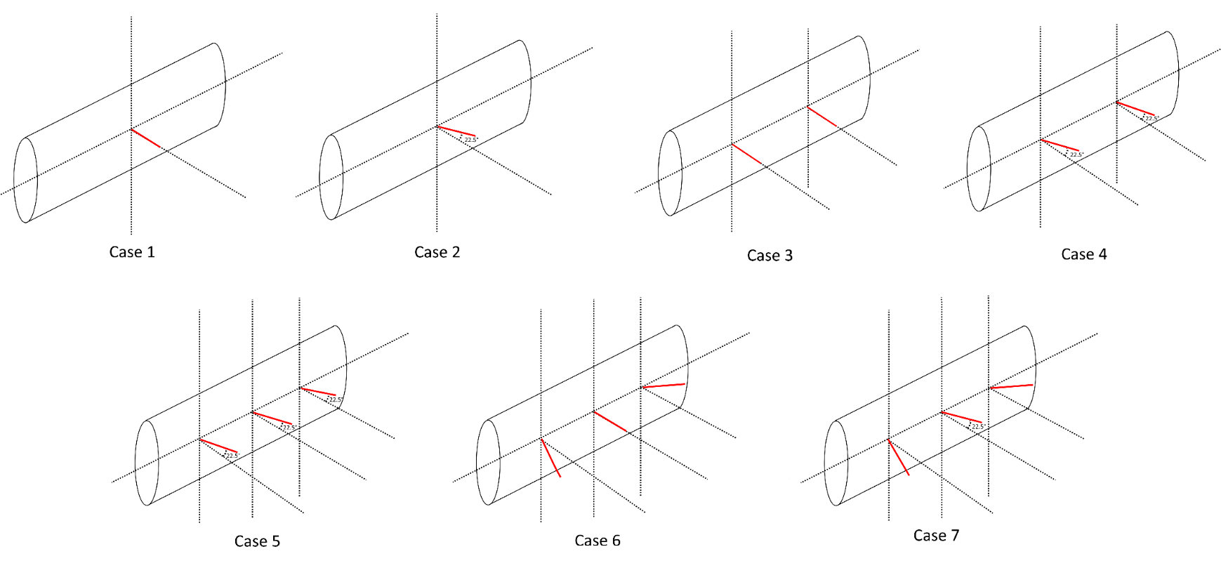
Simulation Hospital challenge
A simulation of the hospital challenge at double speed is shown below. PICO needs to visit cabinets 3, 2 and 0. It looks at its Graph to plan a route through checkpoints to the first cabinet. Everything works just fine for the first cabinet. This is done for the second cabinet as well, but upon arriving at a closed door, it stops. PICO recognizes that it cannot continue with its plan, and plans another route through the corridor by deleting a connection of the Graph and again calculating the shortest path. Furthermore, to know where PICO is, it constantly looks at all the corners it percepts with its laser range finder and fits them on its map (see the section Localization). This way, PICO is able to autonomously navigate through the hospital.

Testing prior to the Hospital challenge
Since the hospital map was known a priori, during the last week of testing on PICO the hospital map was built on the robocup field. During the testing hours, PICO was able to complete a simplified challenge, as there were no obstacles present on its route. The route used can be seen below.
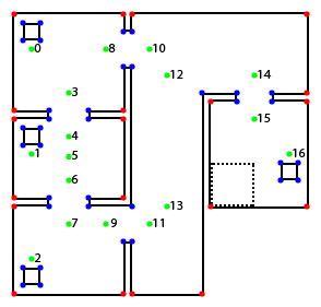
PICO is assigned to visit cabinets 2 and 1. PICO initially orients itself, making sure it knows where it is. PICO now calculates a route towards cabinet 2. If the route is calculated, PICO rotates towards the first checkpoint (15), moves through the door towards checkpoint 16, and turns towards checkpoint 10.
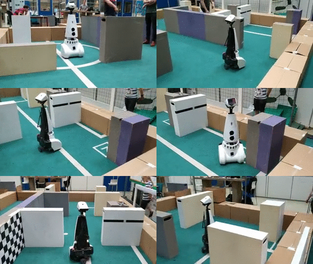
PICO drives towards checkpoint 10, and drives through the second door towards checkpoint 8. It corrects itself once it comes too close to the doorpost, and rotates and moves towards checkpoint 3. Checkpoint 3 was introduced to make sure PICO does not drive into cabinet 2 when it comes from checkpoint 8.
PICO rotates towards checkpoint 0, which is the checkpoint at the first cabinet. As can be seen, its margins are a bit off, but when it reaches the cabinet, it plans a new route towards cabinet 1, and once the route is planned, it rotates towards the next checkpoint (3), and drives towards it.
PICO drives through the door, again correcting itself when it comes too close to the doorpost, towards checkpoint 4, 5, 6, and 7 which are all in a straight line, so it does not need to rotate. Then, it rotates towards checkpoint 2, which is the checkpoint at the second cabinet. When PICO reaches the final cabinet, it turns off.
Results Hospital challenge
The hospital challenge was the final test for PICO and us to check whether the software could handle the imperfections of the real world. In the simulation, PICO is able to succesfully visit cabinets on the given map in any arbitrary order. It was also able to avoid obstacles and re-plan its route when e.g. a door was closed.
During the first try of the Hospital Challenge PICO oriented itself, planned its route towards the first cabinet and drove towards the door of the first room, into the hallway.
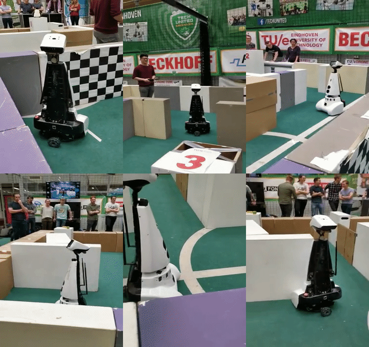
PICO did not care about the dynamic obstacle, since it was not in its direct path, and therefore kept going towards its next checkpoint, at the corner of the corridor. Then, PICO drove past the obstacle with a slightly smaller margin than expected, but still avoiding collision with the obstacle. As can be seen, PICO then does not turn towards the door when it passes by it. It moves towards the wall, since its localization is not correct and therefore it does not know where it is. When PICO arrives at the wall, it turns 180 degrees and moves backwards towards the corridor, trying to localize again. Unfortunately this is not done correctly, and therefore PICO drives into a wall.
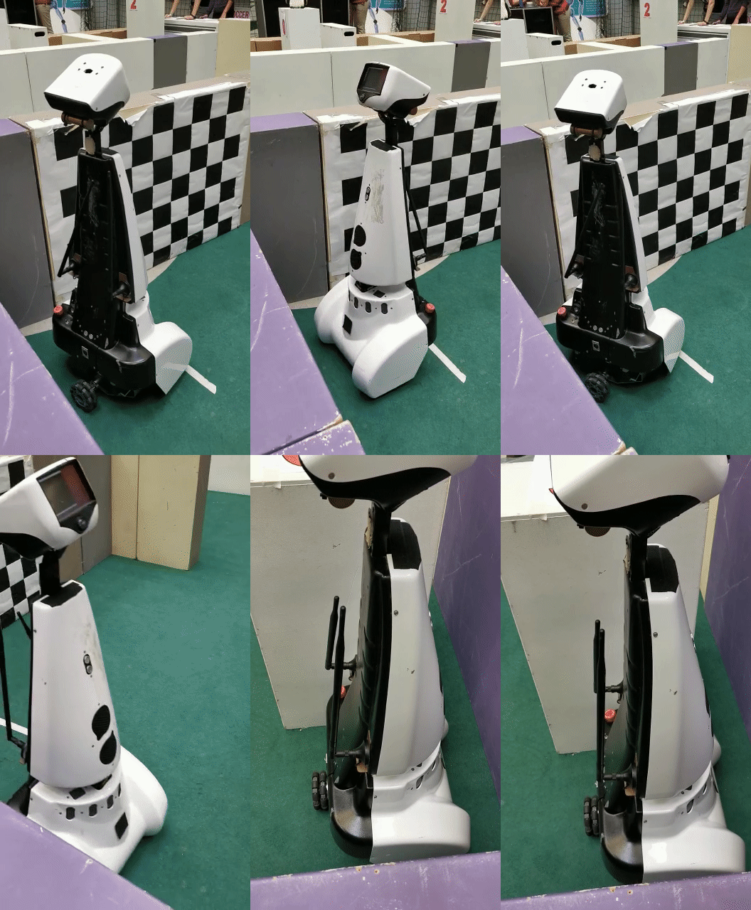
After try 1, at our request, the obstacle was removed from the corridor. This would have made the localization for PICO much more likely to succeed, as it did as such in the simulations. When starting PICO again, we did not hit 'pstart' again. This resulted in the odometry data not being reset, and therefore resulting in the orient controller not working correctly. As can be seen below, PICO did not localize correctly, and drove towards the 1st cabinet instead of its route towards cabinet 0.
Learning points
The following points have been valuable lessons in this project:.
- Although the software architecture is very intuitive to use and of a modular nature, it is quite prone to user errors. As every event and state requires an ID, this becomes cumbersome as the complexity of the plan increases. In the future, it is much wiser to let the software number the components in the order that they are entered. To connect states together, unique strings could be used.
- The plan state machine has grown to be rather complex. Although this does not introduce any complexity in the code, because of the modular design of the software architecture, it is hard to keep an overview even in the conceptual schematic. Instead of introducing a new state for every piece of functionality, one can use a few if statements in function bodies of states. This has to be done with care, as having simple function bodies is one of the key selling points of this software architecture, but keeping the number of states low is advantageous.
- It might have been worth it to use a slightly more complex method to move from checkpoint to checkpoint. Merely checking whether the checkpoint is within a certain distance can lead PICO to miss checkpoints from time to time, requiring it to rotate all the way back and drive towards the checkpoint again. Essentially, we loved simple solutions for most problems but in this case we could have been more careful not to oversimplify it.
- As the software architecture is an important part of the project, it is recommended in the future to have multiple people involved in its design. This makes it easier to implement structural improvements.