Embedded Motion Control 2019 Group 5: Difference between revisions
| Line 205: | Line 205: | ||
== Challenge Strategy == | == Challenge Strategy == | ||
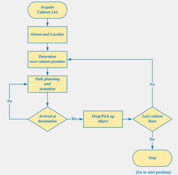
[[File:team5_2019_escape_room_state_diagram.jpg | right | thumb | 500 px | Figure 11: Escape Room State Diagram]] | |||
Two strategies were experimented with to complete this challenge: following the walls till and exit is located, and searching for the exit and driving towards it. While the former sounded easier to implement at the initial stages of discussion (as seen in our Initial Design Document), it was clear that the latter was the faster strategy of the two. In the end a combination of the two strategies was implemented to serve as a fail safe mechanism in case Pico was not able to find an exit within a fixed number of attempts. This section describes the implementation of these two strategies in the Planning Module, while all other modules remain the same. | Two strategies were experimented with to complete this challenge: following the walls till and exit is located, and searching for the exit and driving towards it. While the former sounded easier to implement at the initial stages of discussion (as seen in our Initial Design Document), it was clear that the latter was the faster strategy of the two. In the end a combination of the two strategies was implemented to serve as a fail safe mechanism in case Pico was not able to find an exit within a fixed number of attempts. This section describes the implementation of these two strategies in the Planning Module, while all other modules remain the same. | ||
Revision as of 21:56, 21 June 2019
Welcome to the Wiki Page for Group 5 in the Embedded Motion Control Course (4SC020) 2019!
Group Members
| Name | TU/e Number |
|---|---|
| Winston Mendonca | 1369237 |
| Muliang Du | 1279874 |
| Yi Qin | 1328441 |
| Shubham Ghatge | 1316982 |
| Robert Rompelberg | 0905720 |
| Mayukh Samanta | 1327720 |
Introduction
The world around us is changing rapidly. New technological possibilities trigger new ways of life and innovations like self driving cars, medical robots, are prime examples of how technology can not only make life easier but also safer. In this course we look at the development embedded software of autonomous robots, with a focus on semantically modelling real world perception into the robot's functionality to make it robust to environmental variations that are common in real world applications.
In this year's edition of the Embedded Motion Control course, we are required to use Pico, a mobile telepresence robot with a fixed range of sensors and actuators, to complete two challenges: the Escape Room Challenge and the Hospital Challenge. Our aim was to develop a software structure that gives Pico basic functionality in a manner that could be easily adapted to both these challenges. The following sections in this page detail out the structure and ideas we used in the development of Pico's software, the strategies designed to tackle the given tasks, and our results from both challenges.
Pico
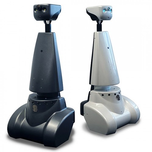
To aptly mirror the structure and operation of a robot deployed in a real-life environment this course uses the Pico robot, a telepresence robot from Aldebaran Robotics. With a fixed hardware platform to work on, all focus can be turned to the software development for the robot. Pico has the following hardware components:
- Sensors/Inputs:
- Proximity measurement with Laser Range Finder (LRF)
- Motion measurement with Wheel encoders (Odometer)
- Control Effort Sensor
- 170-degree wide-angle camera (not used in this course)
- Actuators/Outputs:
- Holonomic Base - Omni wheels that facilitate 2D translation and rotation
- 5" LCD SCreen
- Audio Speaker
- Computer:
- Intel i7 Processor
- OS: Ubuntu 16.04
Functional Requirements for Pico
A description of the expected functionality of robot is the first step to defining its implementation in software in a structured manner. With the given hardware on Pico we were able to define the following functionality for Pico to be able to sufficiently operate in any environment it is placed in:
Generic Requirements
- Pico should be capable of Interpreting (giving real-world meaning) to raw data acquired from its sensors.
- Pico should be capable of Mapping its environment and Localising itself within the mapped environment.
- Pico should be capable of Planning motion trajectories around its environment.
- Pico must adhere to performance and environmental Constraints, such as maximum velocities, maximum idle time while operating, restricted regions, avoiding obstacles, etc.
- Pico should be capable of Providing Information about its operating state and internal process whenever required through the available interfaces.
In addition to these, the following task-specific requirements were defined for Pico (descriptions of the challenges can be found in later sections):
Escape Room Challenge Requirements
- Pico should be capable of identifying an exit and leaving the room from any initial position.
- Pico should use the quickest strategy to exit the room.
- Pico must drive all the way through the exit corridor till the end (past the finish line) to complete the challenge.
Hospital Challenge Requirements
- Pico must be able to accept a dynamic set of objectives (cabinets to visit).
- When Pico visits a cabinet, it should give a clear sound of which cabinet it is visiting (i.e.,“I have visited the cabinet zero”).
- PICO has to make a snapshot of the map once a cabinet is reached.
- PICO should be capable of identifying and working around obstacles and closed doorways while planning its trajectory.
Software Architecture
With the knowledge of the available hardware and the operational requirements for the given tasks, software development can take a well structured and modular developmental approach, thus making it feasible to alter designs and add new functionality at later stages of development. Our software architecture can be split into two parts: the World Model which represents the information system of the robot and the Software Functions which covers all the block that use data from the World Model to give Pico its functionality. While in theory it is encouraged to have a definition of the Information Architecture of system before heading into the Functional Architecture, our software started with the development of a primitive World Model which was later expanded alongside the development of the Software Functions.
World Model
The World Model represents all the data captured and processed by Pico during its operation, and is designed to serve as Pico's real-world semantic "understanding" of its environment. It is created such that software modules only have access to the data required by their respective functions. The data in the World Model can be classified into two sections:
- Environmental Data
- Raw LRF Data
- Interpreted Basic Measurement Information (eg: center, left, right distances; closest and farthest points)
- Detected corner points
- Detected exits
- Processed LRF data in the form of an integer gridmap
- Global Map in the form of an integer gridmap
- Cabinet Locations
- Robot Data
- Operating state
- Localised position
- Desired trajectory
- Odometer readings and offset data
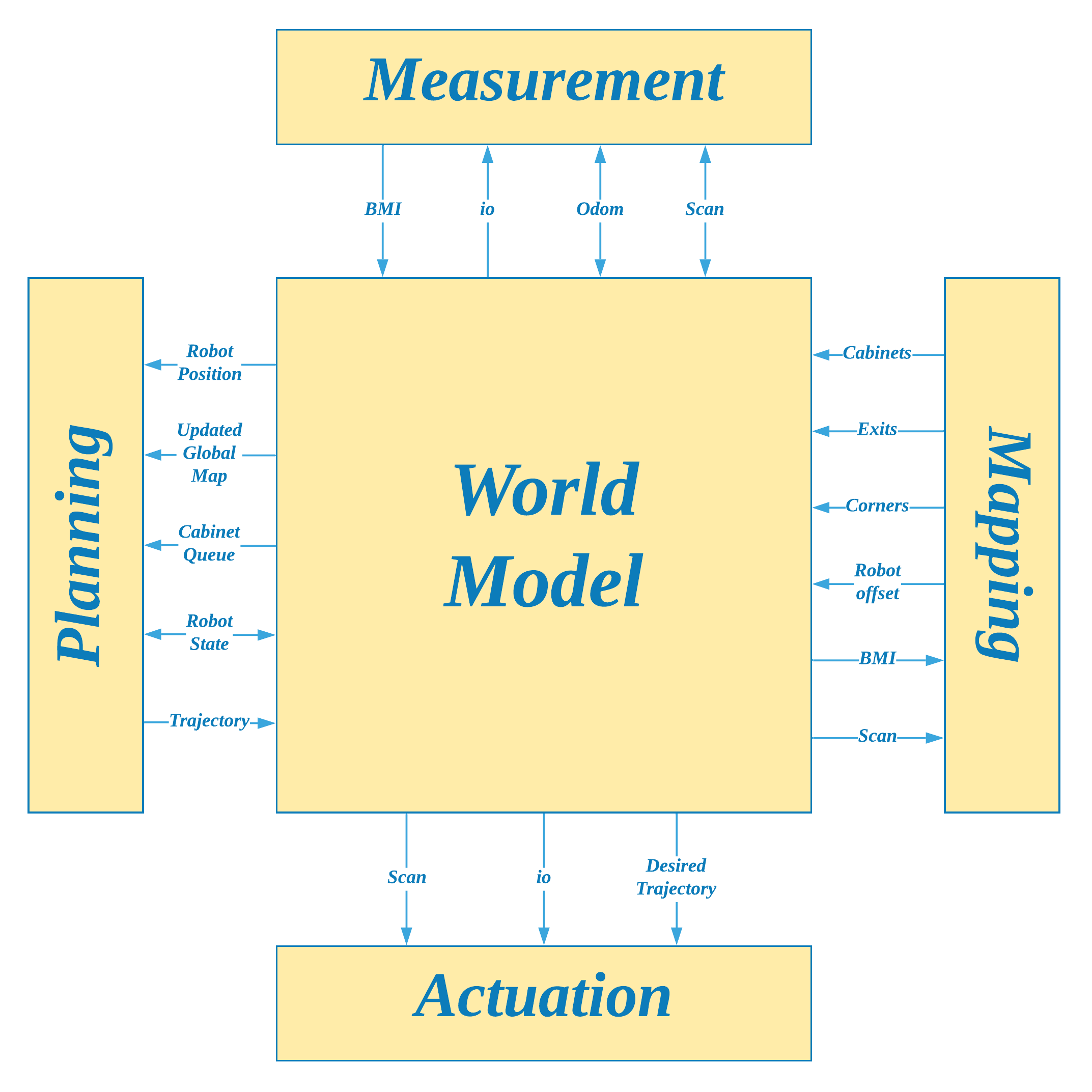
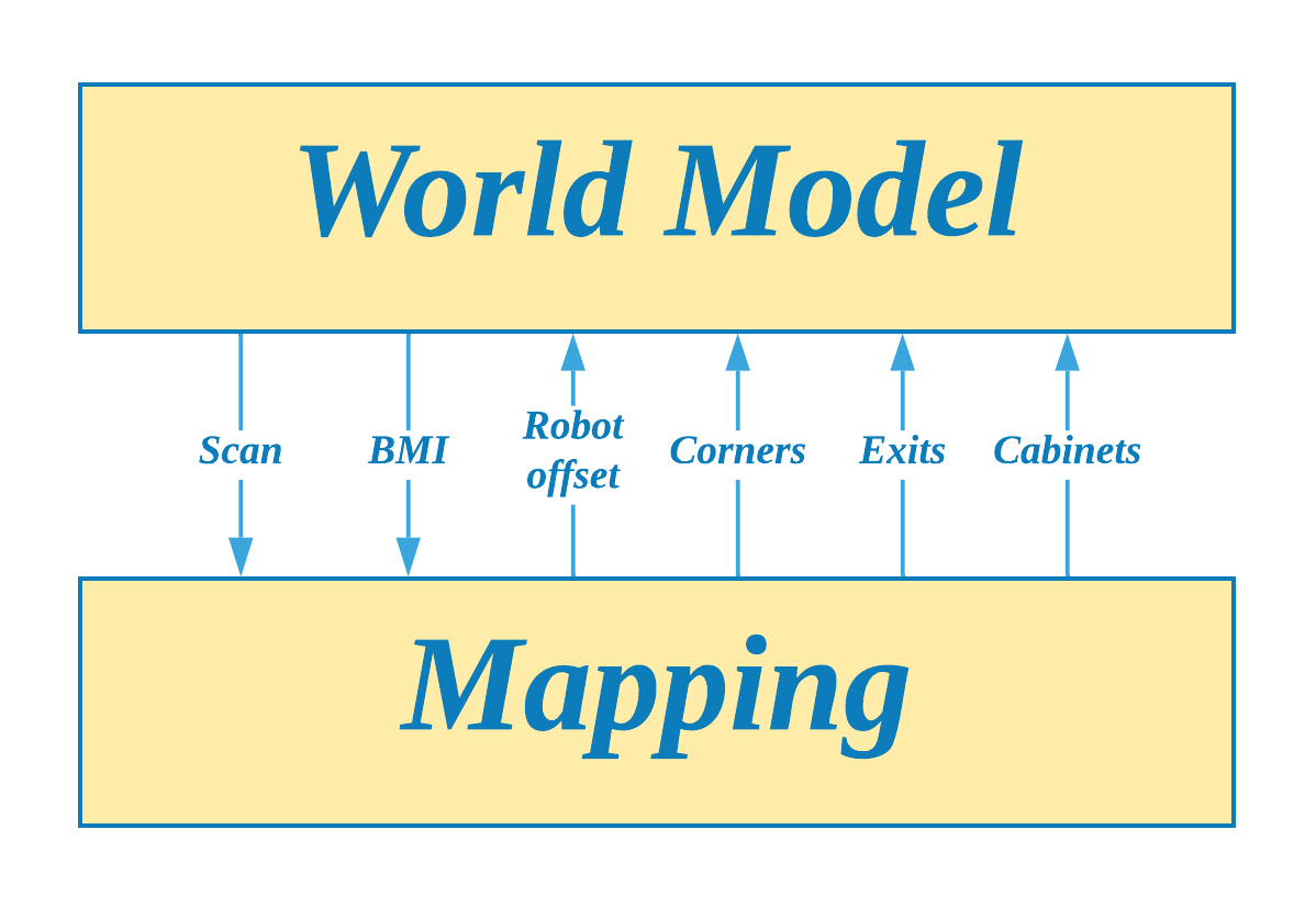
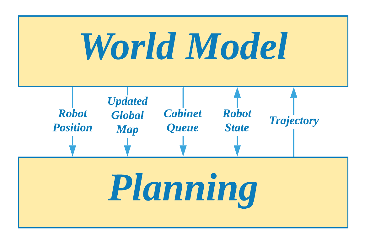
As seen in Figure 1 (click on image to zoom), all parts of Pico's software functions (explained in the next section) interact with the World Model to access data that is specific to their respective operations. To avoid creating multiple copies of the same values and thus optimize on memory usage, each software module accesses its data using references to the World Model, thus asserting one common data location for the entire system.
Functions
This section describes the part of the software architecture that "gives life" to Pico and enables it to perform tasks according to the set requirements. Our software is modularised into four main sections: Measurement, Mapping, Planning and Actuation. As seen from their titles, each section is meant to cover a specific set of robot functions, similar to the organs in a living organism, which when put together with the World Model provide for a completely functional robot. In comparison with the paradigms stated in the course, this structure can be seen as a slightly modified version of the Perception, Monitoring, Planning and Control activities; the functions of Perception are covered by the Measurement and Mapping modules, and Monitoring and Control is covered within the Actuation module. Regardless of these differences, both structure provide the same end result in terms of robot functionality and in terms of being sufficiently modularised. The following sections describes each one of these sections and their corresponding functions, along with a list of some common shared functions at the end.
Measurement
The Measurement module is Pico's "sense organs" division. Here, Pico can read raw data from its available sensors and process some basic information from the acquired data. Figure 2 shows the information interface between the World Model and the Measurement model. The following functions constitute the Measurement Module:
measure()
Reads and processes sensors data into basic measured information
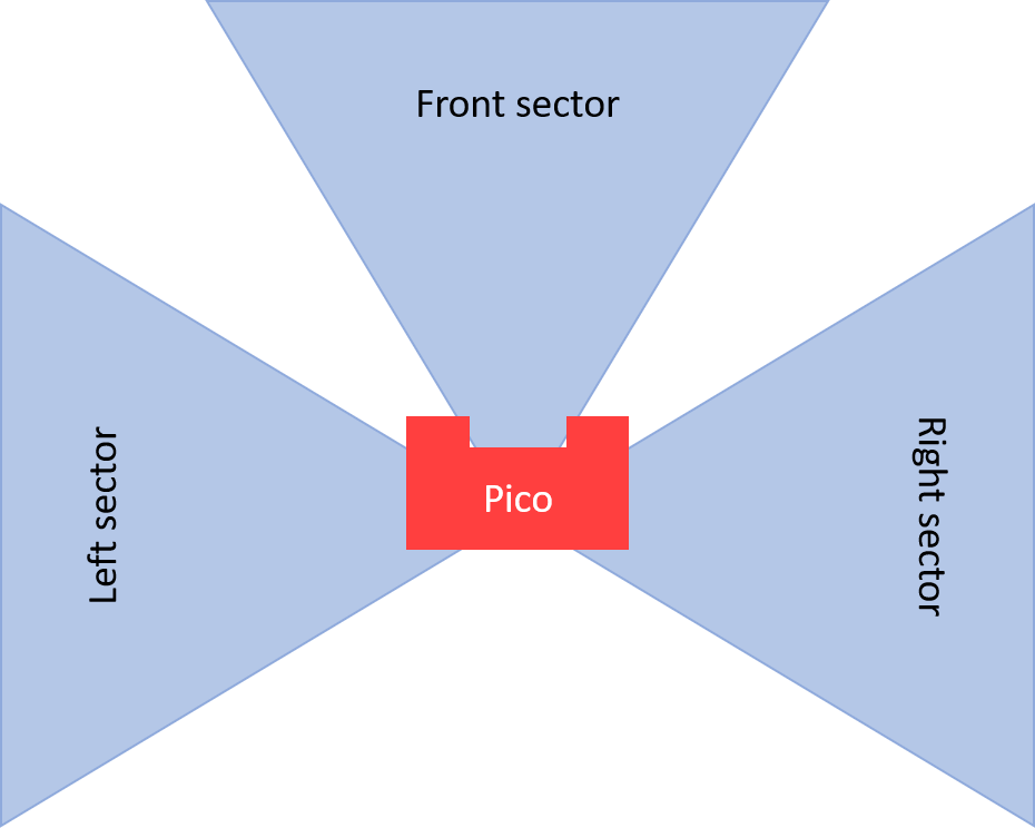
Apart from the standard library functions to read raw data from Pico's LRF and Odometry sensors, the measure() function also interprets and records some primitive information from the obtained LRF data such as the farthest and nearest distances in Pico's current range, the distances at the right, center and left points of the robot, boolean flags indicating whether the right, center or left sectors (sectors are determined by a fixed angular deviation from a given mid point) of Pico's visible range are clear of any obstacles/walls (Figure 3). All these are stored in the World Model to be processed by any other functions that may need this data. Additionally, the measure() function also returns a status check to its parent function, which would indicate whether it was able to successfully acquire data from all sensors, or if not, which sensors failed to deliver any measurements. This would signal Pico to act accordingly in the event of consistent unavailability of data from its sensors. The measure function is the first function to be called in Pico's execution loop.
sectorClear()
Indicates the presence of obstacles/walls in the vicinity of a given heading angle
This function is used to check whether there are any obstacles in a given direction of the robot. While Pico's path planning module is responsible for determining a path devoid of any obstacles, it cannot be guaranteed that Pico would respond exactly according to the planned path or that obstacles around it would stay static while it navigates around them. In this case the sectorClear() function can be fed with Pico's heading angle and thus be used to determine whether the coast is clear of if Pico needs to operate with caution on the current planned trajectory.
alignedToWall()
Determines the deviation of Pico's current heading with respect to a straight wall on the right, left or front of Pico
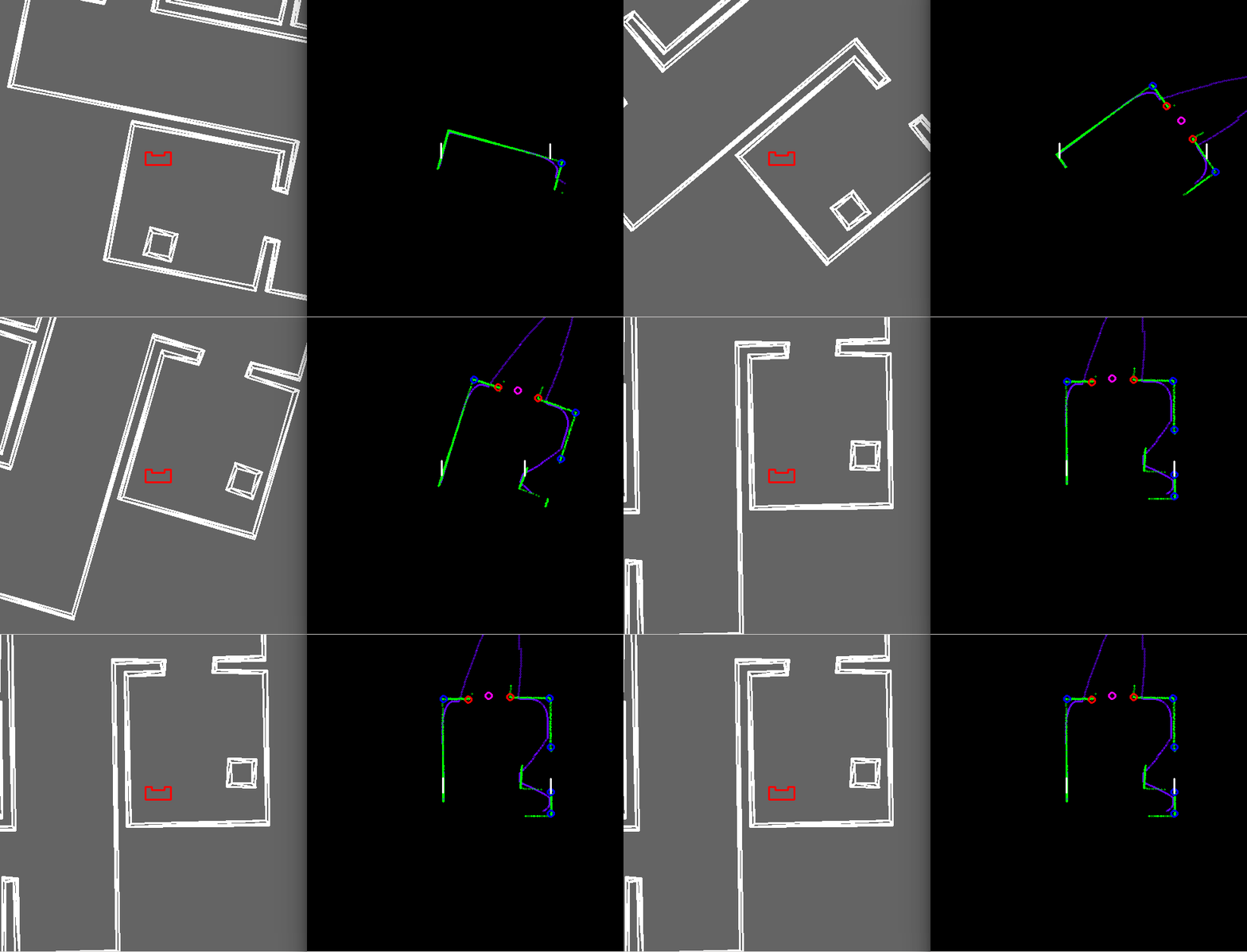
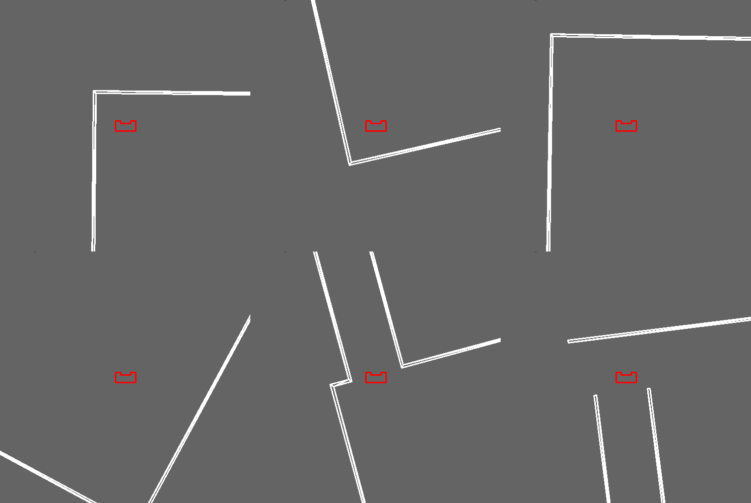
The alignedToWall() function measures the deviation of Pico's right, left or center LRF values from an expected parallel wall. This function is mainly used while localising Pico, to ensure Pico is oriented in a specific pre-determined orientation to obtain its position with respect to a given map. The animation in Figure 4 shows how this is used to rotate Pico till it is aligned to wall on its left; the white vertical lines on the right and left of Pico are used as a reference to compute the alignment difference.
Mapping
Mapping of Pico's environment can be handled in two mutually exclusive scenarios: one where no global map is provided and Pico thus needs to understand its surroundings all by itself, and one where Pico has a global map and can compare its sensed data with the information provided on the map. The Mapping module therefore has two primary functions named identify() and localise() which are responsible for giving Pico a clear understanding of its environment and thus help it determine its actions based on this understanding. The Mapping module also includes several other functions that allow Pico to read and interpret provided maps, generate mapped grid spaces out of the provided map and its sensor data to be used by localise() and other path planning functions, and create visualizations on its screen of processed sensor data. As was with the Measurement module, the Mapping module also interacts with the World Model as its data bank as shown in Figure 5.
identify()
Identifies significant points such as corners and exits in Pico's vicinity
This function uses the acquired LRF data and processes it to identify significant features such as corners, and exits. While this operation is mainly used in situations where Pico does not have access to a global map, this function is also utilised to identify Pico's environment at the start of its run time in order to perform an initial "offset localisation" (explained in the Hospital Challenge section) before it can continue localising with the localise() function. The identify function uses a modified averaging comparison technique to smoothen the obtained noisy LRF data and subsequently compare the averaged data with the original LRF sequence to identify corners. This method also helps it distinguish between convex (red circle) and concave corners (blue circle) as seen in the animation in Figure 4. As several adjacent LRF points would satisfy the condition for identifying corners, all identified corner points are then clustered into single corner points by means of comparing their positions within the LRF sequence. Furthermore, by comparing the distance between two convex corners and the LRF values of distances between those two corners, this method can also identify an exit/entry point (magenta circle) within a room.
localise()
Identifies Pico's current location within a given global map
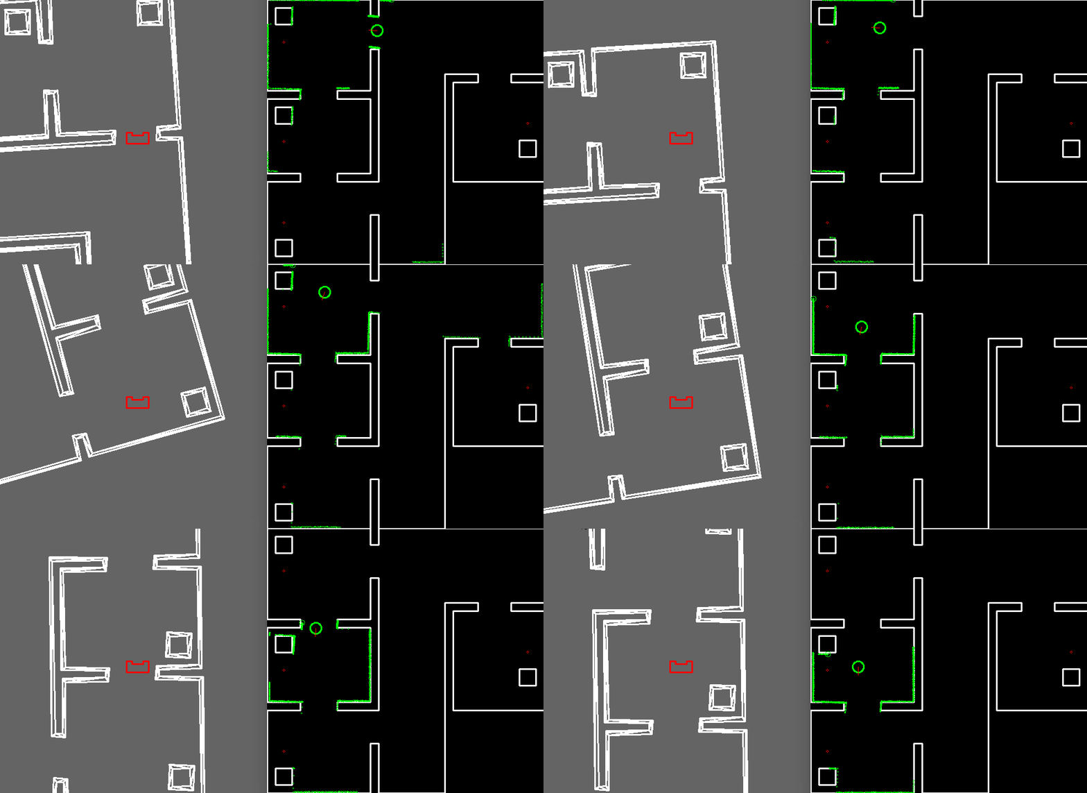
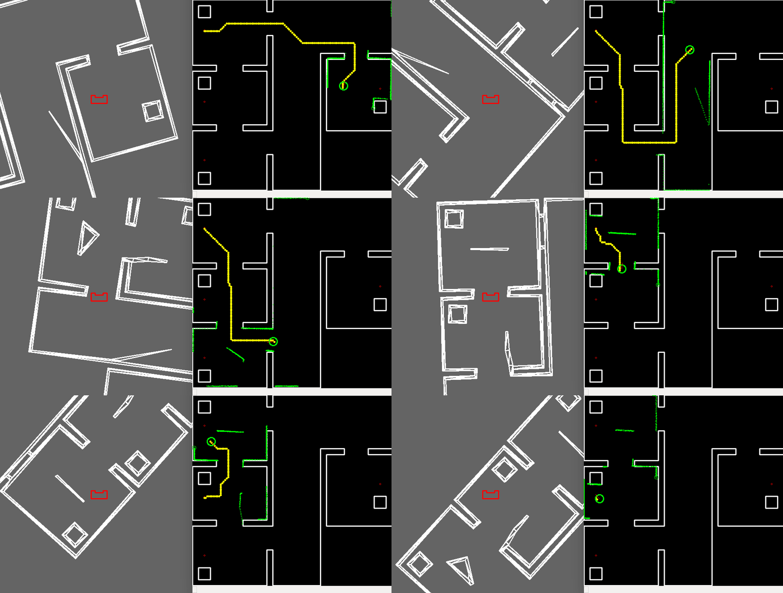
The localise() function uses a minimum difference based cost comparison technique to compare Pico's local map with the global map and thus obtain its position on the global map. This method however relies on an approximate knowledge of Pico's whereabouts on its global map, around which it performs its cost comparison. This approximate position is typically obtained after processing information from the identify() function at Pico's startup or from a combination of Pico's previously localised position, its odometry readings and any error offsets at any stage in execution after the startup. This reliance helps avoid requiring to compare Pico's local map with all possible positions on the global map, thus allowing for a local optimization of possible positions which saves on computation time.
The cost function is computed by assuming the robot to be at a given position on the global map, projecting the LRF points with respect to this position onto the global map and calculating the summation of distances of all LRF points from the closest corresponding point on the global map. The identify() function computes the cost function of several deviations with respect to the approximate location of the robot and thus obtains the position with the least cost as the actual position of the robot on the global map. To further optimize on computation time, the function can also be tuned to project intervals of LRF points onto the global map instead of all available points thus reducing the total number of distance comparisons to be made. A sample of Pico moving around and localising itself is shown in Figure 7.
This method also works in the presence of real-world objects that are not found on the global map, as such points corresponding to obstacles would result in a uniform increase in cost function across all considered position deviations in the optimization process. Additionally, the identify() function evaluates the persistence of these obstacles, and subsequently adds any persistent differences between the local and global map onto the global map which helps in planning paths around closed doors (Figure 8) and also improves the localisation performance as Pico moves through its environment. More results of localisation can be seen in the animations provided in the Hospital Challenge section.
genWeightedMap()
Converts the standard binary global grid map into a weighted integer grid map
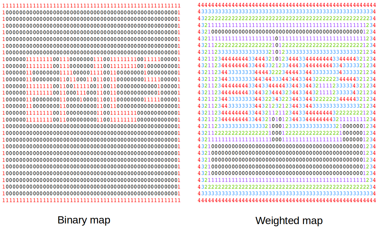
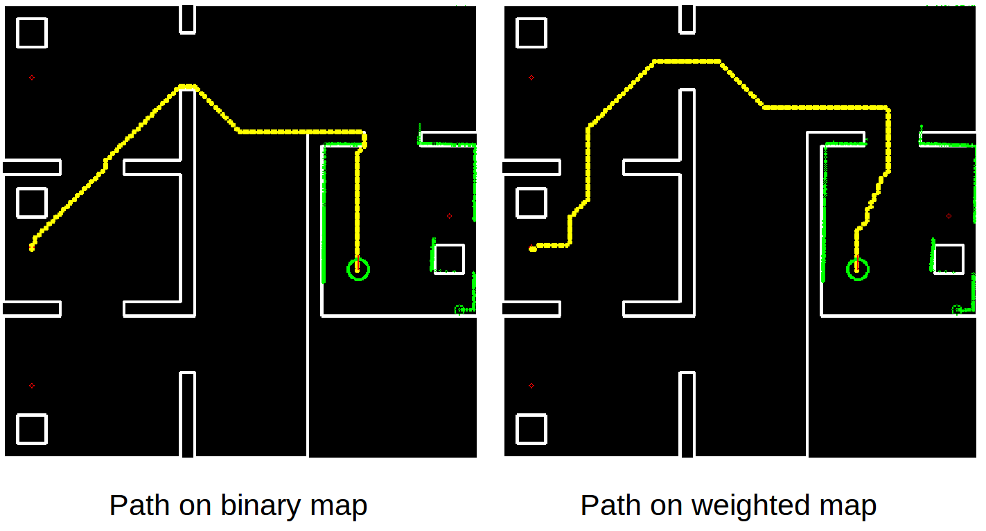
Our solution to navigate around a pre-mapped environment is implemented through the A* Path Planning algorithm which uses a grid map to plan a trajectory between two points on the given grid. With a given global map that has all significant points and walls defined, generating a binary gridmap is a straightforward process. However, the A* algorithm, which tends to select the quickest path available, would generate path that would tend to stick quite close to the walls. Considering that the cell size of the grid map is far smaller compared to Pico's physical dimensions, this would lead to several clashes between any obstacle avoiding functions and the provided path from the path planner. To avoid this, the global grid map is converted from its binary form into a weighted integer form, where the cells with walls and other objects take the highest weights and cells surrounding these have linearly decreasing weights as you go further away from the objects. This additionally allows the path planner to generate paths that drive Pico away from such objects, even if it starts close to them. Figure 8 shows an example of such a conversion, and Figure 9 shows the difference in paths generated with and without the weighted grid map.
Planning
Planning forms the core of Pico's decision making abilities. This module is the main control center of all of Pico's activities, and it governs the way all other modules operate. It comprises one primary function named plan() that essentially operates in the form of a finite state machine. Based on the given task, several operating states are defined, and Pico is made to track its current operations through a state variable. The plan() function uses the information processed by the Measurement and Mapping modules and any previous pieces of information to determine Pico's actions based on the operating state, and delivers this data into the World Model. The most typical actions generated by the plan() function are desired velocity profiles which can be used by the actuation module in the next stage of the operating loop. Figure 9 shows the interaction between the Planning module and the World Model.
Since Pico's operations are dependent on the task it has to perform, Planning is the only module that needs to change to accommodate the differences in functionality requirements between the Escape Room Challenge and the Hospital Challenge. Thus, the states and functions within each state of the planning block are described in the sections specific to each challenge.
Actuation
The final module of the software architecture is the Actuation Module. This module is concerned with the physical control and monitoring of Pico based on instructions received from the previous modules through the World Model as shown in Figure 10.
Actuation::actuate()
Governs the actuation of Pico's Holonomic Base using desired velocity profiles and sensing data
This function takes in inputs in the form of desired translational and rotational velocity profiles, and simply actuates Pico's motors based on these values. To allow for smooth motion profiles, the actuate() function also tracks Pico's current velocity and incrementally adjusts it match the desired velocity from the world model. Additionally, the actuate function also employs obstacle avoidance by computing Pico's heading based on the desired velocity vectors and adjusts its actual velocity to either move away or to move slowly if it finds an obstacle in the vicinity of its heading.
Additional Functions and Software Features
The above modules cover the main functionality of Pico to complete the task at hand. These modules are further supplemented by some additional common resources and software features that either aid in the operation of the primary functions or are useful for debugging of the software.
- Json to Binary map: This function generates a binary map grid map from the provided global map in JSON format, with room and cabinet walls represented by a 1 and empty spaces represented by 0s.
- Performance Variables: As stated in the requirements, Pico must adhere certain performance constraints. These are listed out in the form of Performance structure that contains information such the maximum and minimum permissible velocities, minimum permissible distance, minimum measurable distance, etc.
- Data Logging: Through this logging feature, Pico is able to log all important processed information based on its operating state into files that can be analysed for performance later. Each module manages its own separate log, and log messages can also be displayed on a console in real-time while Pico operates.
- Module Enable Flags: An additional testing and debugging feature is a set of enable flags that allow the user to temporarily switch off one of the modules. This, for example, is useful in instances where the user may want to manually control Pico for testing purposes while it continues to measure and map its environment.
Escape Room Challenge
The first competition in this course was the Hospital Challenge. The main objective of this challenge is for Pico to be able to locate the exit of a room whose dimensions are not known before hand (no map provided) from any starting position within the room and subsequently exit the room as quickly as possible. A detailed description of this challenge can be found here.
Challenge Strategy
Two strategies were experimented with to complete this challenge: following the walls till and exit is located, and searching for the exit and driving towards it. While the former sounded easier to implement at the initial stages of discussion (as seen in our Initial Design Document), it was clear that the latter was the faster strategy of the two. In the end a combination of the two strategies was implemented to serve as a fail safe mechanism in case Pico was not able to find an exit within a fixed number of attempts. This section describes the implementation of these two strategies in the Planning Module, while all other modules remain the same.
Primary Strategy: Scan For Exit
In this strategy, Pico makes use of the corner and exit detection features in it Mapping Module to be able to determine whether or not it sees an exit in its current field of view. If an exit is currently not visible, Pico starts to rotate through a fixed angle, while still looking for an exit. If at the end of this rotation maneuver Pico is still unable to find the exit, it is probably in a corner of the room where a clear view of the exit is obscured from its sensing range. In this case, Pico translates forward for a fixed length and continues to look for an exit during this motion too. At the end of this motion if an exit is still not found, Pico repeats the rotate and translate for a maximum of four tries, after which it indicates that it is unable to find the exit through this strategy and subsequently switches to the Wall Following strategy. In tests with different exit positions and robot initial positions, it was found that Pico never needed to switch to the Wall Following startegy and was always able to find the exit within three iterations of rotating and translating. On encountering an exit during any of these previously mentioned operations, Pico switches its operational state to face and drive towards the exit. Upon reaching the exit, Pico then orients itself to be parallel to the exit corridor and goes on to perform a corridor/wall follow maneuver till it has left the corridor. All these operations are described in the state diagram shown in Figure 11.
Secondary Strategy: Wall Following
In this backup strategy, Pico uses the walls of the room as a guide to eventually reach the exit. Pico would begin by locating the nearest wall to itself, driving towards it and aligning itself to be parallel to the wall. After this it runs in a continuous loop of driving parallel to the wall until it detects that it is at a corner (wall ahead of it) or till it detects the exit (large change in distance measured) on the side that it was following the wall. In the event of detecting a corner, it would perform a 90 degree turn in the direction of the corner, align itself to the wall and continue following it as before. If it detects an exit it would instead turn towards the exit and carry out a corridor/wall follow maneuver till it has left the corridor.
End Result and Future Improvements
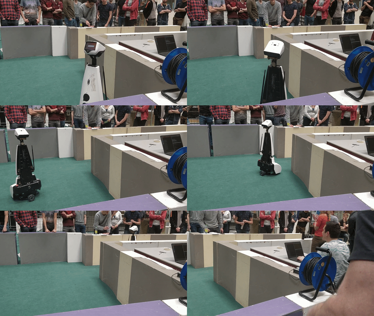
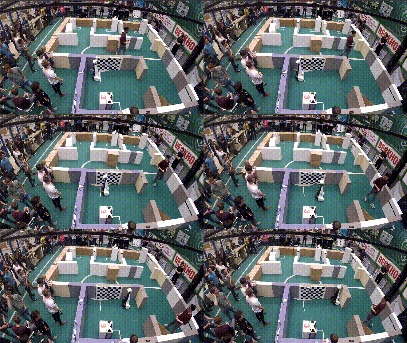
In the first attempt at the Escape Room Competition (Figure 12), Pico performed as expected by looking around for the exit, driving forward on not seeing it initially, eventually detecting the exit and heading towards it. However it seemed to drift sideways while arriving at and while subsequently entering the exit corridor. This caused it to slightly bump into the exit wall at the start of the exit, but it eventually corrected itself and crossed the exit corridor. To temporarily avoid this bumping its maximum translational velocity was lowered for the second attempt, wherein it exhibited the same sideways drifting behaviour, but was able to stop short of bumping into the wall. With this we were able to complete the challenge in the quickest time of about 40 seconds and thus rank first in this competition!
On inspecting the code later, a logical bug in the actuation module was found to be responsible for the sideways drift. This was fixed to achieve an output as seen in the simulation in Figure 13.
Another small aspect that could have further lowered the time Pico took to complete the challenge was the pauses between each operational state. In order to observe Pico's actions and comprehend them while they were taking place, a one second delay was added to Pico's operation every time it switched form one state to another. Eliminating this delay could have lowered the overall operational time by 6 seconds.
Hospital Challenge
The Hospital Competition is the second part of this course. In this competition, Pico must navigate around a fixed hospital environment with help from a provided global map, with the aim of visiting specific sites (cabinets) while avoiding any static or dynamic obstacles and closed doors. A detailed description of the Hospital Challenge can be found here.
Challenge Strategy
Our solution to the Hospital Challenge used a relatively smaller strategy as compared to the Escape Room Challenge. Pico begins operation by accepting a list of cabinet numbers that it should visit. Before it can attempt to move anywhere, it must first localise itself within the provided global map. To do this, Pico makes use of the known features of the room such as the exit and the room corners detected by the identify() function of the Mapping Module. It starts by aligning itself parallel to the left wall of the room and then comparing the position of the detected exit with their corresponding positions on the global map to obtain its starting position. From here on, Pico gets the first/next cabinet in the previously acquired list of cabinets, plans a trajectory from its current position till the cabinet using the A* Path Planning algorithm and goes on to follow this trajectory, while updating the global map with any differences from its sensed local map. On reaching a cabinet, Pico performs a fixed routine of orienting itself to face the cabinet, taking a snapshot of its current LRF data and finally announcing its arrival at that cabinet via its speaker. It then proceeds to get the next available cabinet on the list in the same manner as above and continues this process till all the cabinets in its list have been visited. Figure 13 shows the state diagram of the Planning module to carry out the above series of operations.
End Results and Future Improvements
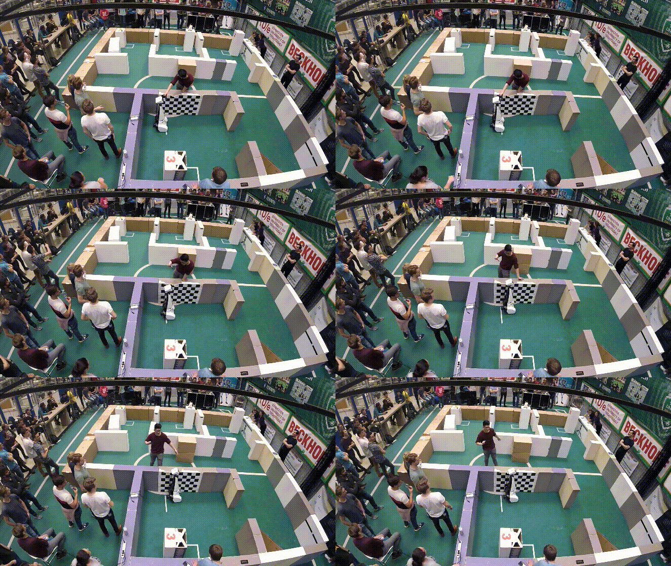
Unfortunately, the Hospital Challenge competition did not go as expected (Figures 14 and 15). In the first attempt, Pico drove towards the exit of the room, but deviated from its path midway and collided with the left wall of the room. In the second attempt, Pico had a similar result wherein it immediately drove towards the left wall. On examining the log files from both runs and attempting to run Pico again once the competition was over, we were able to find that an error in the localisation made Pico believe that it was instead facing the right side of the room consequently leading it to believe that the entire map was rotated by 90 degrees in the counterclockwise direction, thus resulting in the drive towards the left wall. This was later fixed and the results of the same are shown in the simulations in Figures 14 and 15.
