Football Table Simulation Visualization Tool: Difference between revisions
| (15 intermediate revisions by one other user not shown) | |||
| Line 5: | Line 5: | ||
drawing for more complex geometry. A previous attempt was created using [http://www.openrobots.org/wiki/morse MORSE], however this was aborted because the poor tune-ability of the physics and limited options for communication.</p> | drawing for more complex geometry. A previous attempt was created using [http://www.openrobots.org/wiki/morse MORSE], however this was aborted because the poor tune-ability of the physics and limited options for communication.</p> | ||
<p>A guide on how to build gazebo can be found [http://gazebosim.org/wiki/1.6/install#Compiling_From_Source here], the latest version that has been tested is 1.8.3 and can be found on the svn. Make sure to source the <code>setup.sh</code> located on the svn, instead of the one that comes with gazebo. </p> | |||
[[File:Gazebo.png|thumb|center|upright=4.0|The gazebo simulator for the semi-automated soccertable.]] | [[File:Gazebo.png|thumb|center|upright=4.0|The gazebo simulator for the semi-automated soccertable.]] | ||
==Synchronized Inter-process Communication== | ==Synchronized Inter-process Communication== | ||
<p> | <p> | ||
To date, Gazebo is mostly used in combination with [http://wiki.ros.org/ ROS. However using ROS plugins yields a lot of overhead, moreover the timers and communication provided there or not accurate enough to ensure an accurate casual link. Therefore a plug-in was created enabling fast light-weight inter-process communication, allowing to run simulation to be ran up to 20 times faster than real-time without loss of causality. | To date, Gazebo is mostly used in combination with [http://wiki.ros.org/ ROS]. However using ROS plugins yields a lot of overhead, moreover the timers and communication provided there or not accurate enough to ensure an accurate casual link. Therefore a plug-in was created enabling fast light-weight inter-process communication, allowing to run simulation to be ran up to 20 times faster than real-time without loss of causality. | ||
</p> | </p> | ||
| Line 16: | Line 18: | ||
</p> | </p> | ||
<references /> | <references /> | ||
==Building the libraries/plugins== | |||
<p>After building gazebo and its requirements, you can build all libraries used for RL/IPC. These can be build by running the <code>src/shm_ipc/install.sh</code> and <code>/src/rl/install.sh</code>.</p> | |||
==Matlab Simulink== | ==Matlab Simulink== | ||
<p>The Simulink side of things can be found in <code>MOTION_test.mdl</code>, this is ''not'' an external, but is ran in simulink itself in the regular way. The main window is shown below, the simulator part is the the gazebo sub-system. The motion-generation contains the reinforcement learning, attractor dynamics and constraints for the actions.</p> | <p>The Simulink side of things can be found in <code>MOTION_test.mdl</code>, this is ''not'' an external, but is ran in simulink itself in the regular way. The main window is shown below, the simulator part is the the gazebo sub-system. The motion-generation contains the reinforcement learning, attractor dynamics and constraints for the actions. To start the simulation just press simulation->start. If you want to view what is going on, open a terminal and type <code>gzclient</code> to start the gazebo GUI.</p> | ||
[[File:MOTION_test.png|thumb|center|upright=1.5| Main window of <code>MOTION_test.mdl</code>]] | [[File:MOTION_test.png|thumb|center|upright=1.5| Main window of <code>MOTION_test.mdl</code>]] | ||
<p>In the motion generation sub-system the ETA (estimated time of arrival) is indicated (how long the simulation will take in minutes). Also the current episode number is displayed.</p> | |||
[[File:MOTION_test_RL.png|thumb|center|upright=1.5| Motion generation window <code>MOTION_test.mdl</code>]] | [[File:MOTION_test_RL.png|thumb|center|upright=1.5| Motion generation window <code>MOTION_test.mdl</code>]] | ||
===Reinforcement learning settings=== | |||
====General==== | |||
<p> | <p> | ||
Most relevant settings regarding the actions and the reinforcement learning are set in their respective masks. In the mask of <code>primitives_select.cpp</code> you can set all the parameters described in [http://cstwiki.wtb.tue.nl/index.php?title=Football_Table_RL#Library_functions this RL section]. | Most relevant settings regarding the actions and the reinforcement learning are set in their respective masks. In the mask of <code>primitives_select.cpp</code> you can set all the parameters described in [http://cstwiki.wtb.tue.nl/index.php?title=Football_Table_RL#Library_functions this RL section].<br/> | ||
In the tab named ''general'' the following settings are available: | |||
[[File:RL_tab1.png|thumb|center|upright=1.0| General settings ]] | |||
;Store Data | |||
:Checkbox to enable the storage of data, this will store the buffers and the performance of the simulation you run. | |||
;Store Policy | |||
:Checkbox to enable storage of the policy. This will store the learned weight vectors <math>\theta,~w</math>, but also other settings such as the node positions (centers), number of states and actions etc. | |||
;Data Path | |||
:Path to the folder in which all data will be stored. A new folder with a timestamped name will be created, also the name of the folder indicates what RL algorithm was used. | |||
;Number of states | |||
:Number of states used as input to the learning agent | |||
;Available states | |||
:Vector with indices of the states, the allow quick changes you can select a couple of seperate states from the input of the simulink block. I.e. we only want the lateral position and speed of the ball. We can then say: Number of states = 2, available states [1 3] indicating index 1 and 3 in the learning state. Make sure to adjust the function approximation accordingly. | |||
;Number of actions | |||
:number of actions available to the learning agent | |||
;Available actions | |||
:Similar to available states, vector with indexes of the actions you want available (0-5). | |||
;Number of samples | |||
:Total of episodes that are done in this simulation until it is stopped. (Make sure the simulation runs long enough in order to finish all of them). | |||
;Number of greedy samples | |||
:Number of episodes in which fully greedy behavior is performed (<math>\epsilon=0</math>). If this is the same as the number of samples, then only greedy behavior will be performed. | |||
</p> | </p> | ||
====Learning parameters==== | |||
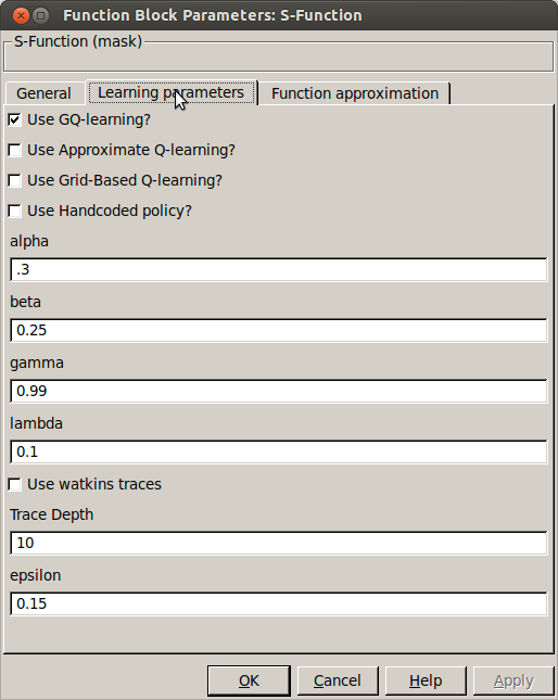
[[File:RL_tab2.png|thumb|center|upright=1.0| RL settings ]] | |||
;Use GQ-learning | |||
:Use greedy-GQ for updating the value function approximation | |||
;Use approximate-Qlearning | |||
:Use approximate-Qlearning for updating the value function approximation | |||
;Use grid-based Q-learning | |||
:Use grid based function approximation. This is no longer available in the latest version, you can still find in <code>primives_select_old.cpp</code>. | |||
;Use hand-coded policy | |||
:Use a user defined policy, this code is too be defined in primives_select.cpp. An actual handcoded policy can be found in <code>primives_select_old.cpp</code>. | |||
;Alpha | |||
:The learning rate <math>\alpha</math> | |||
;Beta | |||
:The secondary parameter for greedy-GQ <math>\beta</math> | |||
;Gamma | |||
:The discount factor <math>\gamma</math> | |||
;Lambda | |||
:Eligibility trace parameter <math>\lambda</math> | |||
;Use watkins traces | |||
:Use Watkins style traces: cut-off a trace once an non-optimal(/exploratory) action is performed | |||
;Trace depth | |||
:Maximum amount of steps back the trace is updated | |||
;Epsilon | |||
:Exploration rate, the higher it is the more ''random'' actions are performed (not based on value). | |||
====Value function approximation ==== | |||
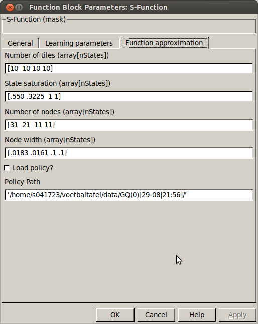
[[File:RL_tab3.png|thumb|center|upright=1.0| RL settings ]] | |||
<p>These settings are parallel to what is explained [http://cstwiki.wtb.tue.nl/index.php?title=Football_Table_RL#Library_functions here]. Make sure the size of these arrays matches the number of states defined in the ''general'' tab. The settings that are not explained [http://cstwiki.wtb.tue.nl/index.php?title=Football_Table_RL#Library_functions here] are:</p> | |||
;Load policy? | |||
:Checkbox indicating whether or not to load an old policy | |||
;Policy Path | |||
:Absolute path pointing to the folder in which the policy files can be found. | |||
Latest revision as of 16:39, 16 May 2019
Author: Erik Stoltenborg
Gazebo
A simulator is developed to easily test new algorithms without depending on the actual robot. In has been developed using gazebo (w/o the use of ROS), a so-called physics abstraction layer, which employs ODE combined with OGRE for rendering. Gazebo has been very well maintained since 2012, since it became the official simulator for the DARPA Robotics Challenge. The environment/robots are described in the SDF format, which is very simular to *.xml. It can be easily combined with CAD-files, in this case is combined with a Collada [1] drawing for more complex geometry. A previous attempt was created using MORSE, however this was aborted because the poor tune-ability of the physics and limited options for communication.
A guide on how to build gazebo can be found here, the latest version that has been tested is 1.8.3 and can be found on the svn. Make sure to source the setup.sh located on the svn, instead of the one that comes with gazebo.
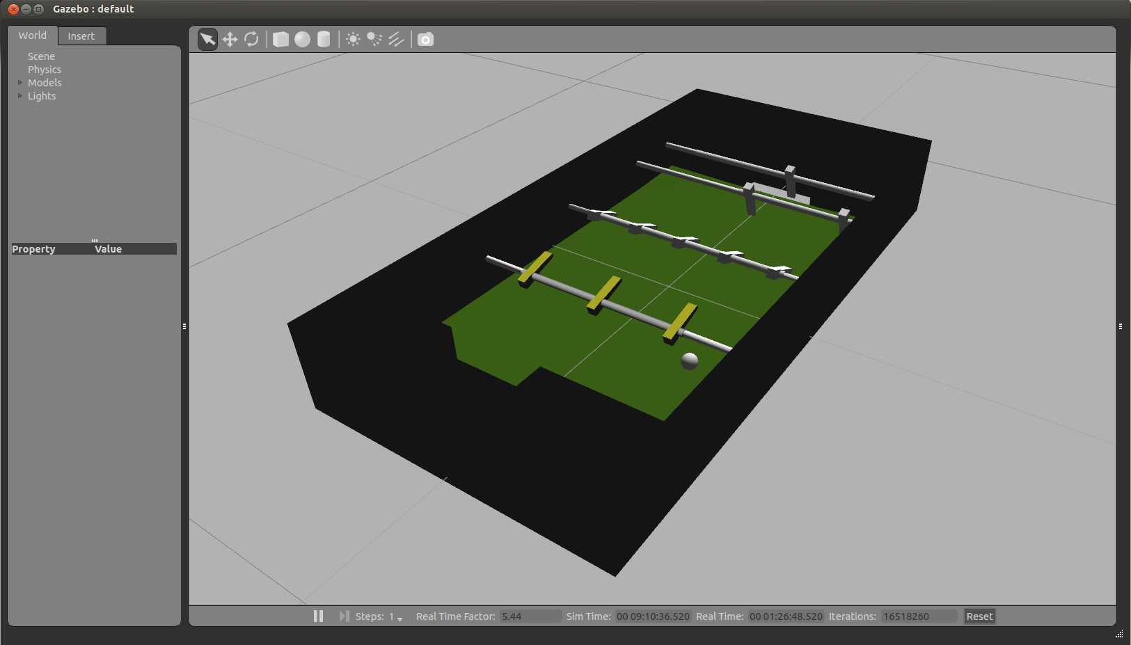
Synchronized Inter-process Communication
To date, Gazebo is mostly used in combination with ROS. However using ROS plugins yields a lot of overhead, moreover the timers and communication provided there or not accurate enough to ensure an accurate casual link. Therefore a plug-in was created enabling fast light-weight inter-process communication, allowing to run simulation to be ran up to 20 times faster than real-time without loss of causality.
This simulation communicates with Matlab Simulink using Interprocess Communication (IPC) wrapper library for the POSIX libraries, the wrapper makes the use of shared memory more accesible and easy to use. It uses shared memory protected by mutexes and condition variables enabling a thread-safe, synchronized, causal communication between two processes e.g. Gazebo and Simulink. This allows us to use the Gazebo simulator as a plant in our simulink control loop. Moreover this wrapper library could be used for (safe) IPC between two arbitrary processes. More on this library, it's basic principles and how it is used can be found here.
Building the libraries/plugins
After building gazebo and its requirements, you can build all libraries used for RL/IPC. These can be build by running the src/shm_ipc/install.sh and /src/rl/install.sh.
Matlab Simulink
The Simulink side of things can be found in MOTION_test.mdl, this is not an external, but is ran in simulink itself in the regular way. The main window is shown below, the simulator part is the the gazebo sub-system. The motion-generation contains the reinforcement learning, attractor dynamics and constraints for the actions. To start the simulation just press simulation->start. If you want to view what is going on, open a terminal and type gzclient to start the gazebo GUI.
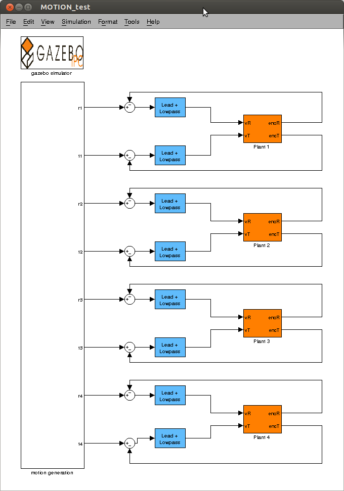
MOTION_test.mdlIn the motion generation sub-system the ETA (estimated time of arrival) is indicated (how long the simulation will take in minutes). Also the current episode number is displayed.
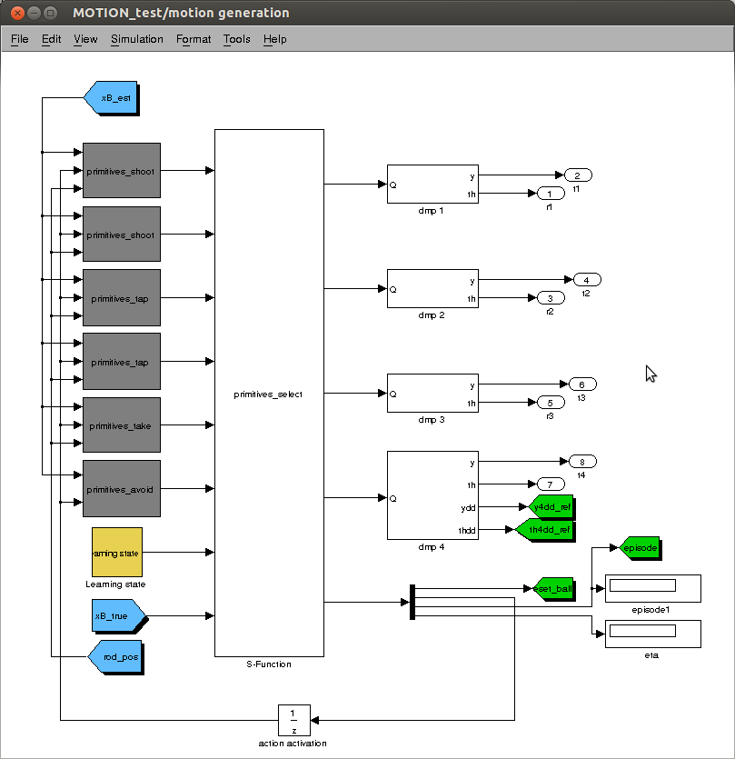
MOTION_test.mdlReinforcement learning settings
General
Most relevant settings regarding the actions and the reinforcement learning are set in their respective masks. In the mask of primitives_select.cpp you can set all the parameters described in this RL section.
In the tab named general the following settings are available:
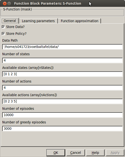
- Store Data
- Checkbox to enable the storage of data, this will store the buffers and the performance of the simulation you run.
- Store Policy
- Checkbox to enable storage of the policy. This will store the learned weight vectors [math]\displaystyle{ \theta,~w }[/math], but also other settings such as the node positions (centers), number of states and actions etc.
- Data Path
- Path to the folder in which all data will be stored. A new folder with a timestamped name will be created, also the name of the folder indicates what RL algorithm was used.
- Number of states
- Number of states used as input to the learning agent
- Available states
- Vector with indices of the states, the allow quick changes you can select a couple of seperate states from the input of the simulink block. I.e. we only want the lateral position and speed of the ball. We can then say: Number of states = 2, available states [1 3] indicating index 1 and 3 in the learning state. Make sure to adjust the function approximation accordingly.
- Number of actions
- number of actions available to the learning agent
- Available actions
- Similar to available states, vector with indexes of the actions you want available (0-5).
- Number of samples
- Total of episodes that are done in this simulation until it is stopped. (Make sure the simulation runs long enough in order to finish all of them).
- Number of greedy samples
- Number of episodes in which fully greedy behavior is performed ([math]\displaystyle{ \epsilon=0 }[/math]). If this is the same as the number of samples, then only greedy behavior will be performed.
Learning parameters
- Use GQ-learning
- Use greedy-GQ for updating the value function approximation
- Use approximate-Qlearning
- Use approximate-Qlearning for updating the value function approximation
- Use grid-based Q-learning
- Use grid based function approximation. This is no longer available in the latest version, you can still find in
primives_select_old.cpp. - Use hand-coded policy
- Use a user defined policy, this code is too be defined in primives_select.cpp. An actual handcoded policy can be found in
primives_select_old.cpp. - Alpha
- The learning rate [math]\displaystyle{ \alpha }[/math]
- Beta
- The secondary parameter for greedy-GQ [math]\displaystyle{ \beta }[/math]
- Gamma
- The discount factor [math]\displaystyle{ \gamma }[/math]
- Lambda
- Eligibility trace parameter [math]\displaystyle{ \lambda }[/math]
- Use watkins traces
- Use Watkins style traces: cut-off a trace once an non-optimal(/exploratory) action is performed
- Trace depth
- Maximum amount of steps back the trace is updated
- Epsilon
- Exploration rate, the higher it is the more random actions are performed (not based on value).
Value function approximation
These settings are parallel to what is explained here. Make sure the size of these arrays matches the number of states defined in the general tab. The settings that are not explained here are:
- Load policy?
- Checkbox indicating whether or not to load an old policy
- Policy Path
- Absolute path pointing to the folder in which the policy files can be found.