Embedded Motion Control 2013 Group 9: Difference between revisions
| Line 338: | Line 338: | ||
*''' Main program flow ''' | *''' Main program flow ''' | ||
The main program flow is depicted below. | The main program flow is depicted below. | ||
[[File: | [[File:Diagram3.jpg|center|800px]] | ||
=== Laser data interpretation and processing === | === Laser data interpretation and processing === | ||
Revision as of 14:22, 22 October 2013
Group members
| Name: | Student id: | Email: |
| Jeroen Lamers | 0771264 | j.w.lamers@student.tue.nl |
| Rens Samplonius | 0785119 | r.j.samplonius@student.tue.nl |
| Haico Ploegmakers | 0775395 | h.e.c.w.ploegmakers@student.tue.nl |
| Frank Evers | 0789890 | f.evers@student.tue.nl |
| Filipe Catarino | 0821789 | f.freire.catarino@student.tue.nl |
| Tutor: |
| Janno Lunenburg |
Planning
| Week: | Activities: | People: |
| Week 1 |
|
* Everbody |
| Week 2 |
|
|
| Week 3 |
|
|
| Week 4 |
|
|
| Week 5 |
|
|
| Week 6 |
|
|
| Week 7 |
|
|
| Week 8 |
|
|
Progress
Week 1: September 2 - September 8
The first week mainly consisted of installing the Ubuntu OS with all the required ROS/Gazebo software. This did not went smoothly as there is no easy available Ubuntu installation for Mac (1 member) and missing one tiny step in the Tutorials could end up with a not working environment.
It was decided that everyone should do all the tutorials to know how everything works, and that we would work with the software provided by the course material (QT for c++ and fuerte Ros).
Week 2: September 9 - September 15
During the second week everyone finished the tutorials for ROS and c++.
Robot Sensors
Researching the given example with the simulation environment shows that the laser data is acquired by scanning in a 270 degree angle with increments of 0.25 degrees. This information is saved in a a vector and can be used to obtain distances for every angle at a certain time.
Week 3: September 16 - September 22
The third week consisted of 2 parts:
- Creating the architecture of the system, by dividing all the necessary steps into functions.
- Focus on the corridor competition
System functions & Architecture
The group was split into two teams where 2 people where focusing on the architecture of the system. By doing this early it is clear how the system is going to be created. There is one main file that is able to call for all different functions that are required for the situation at hand. The focus of course is on the basic functions of the system for the corridor competition. These functions are:
- Driving in a straight line in the middle of the corridor
- Detecting the corner on either the left or the right side
- Turn into the corner and leave the corridor
- Stop outside the corridor
Corridor Competition concept
Because the contest dictates that the robot will be between the walls, and facing the end of the competition, the idea is that the robot is able to drive forward into the corridor. Because the robot is put there by human hand, and walls might not be exactly parallel there has to be some kind of control. By measuring the closest distance to the walls with the laser, the robot is able to calculate where the middle of the corridor is. The laser is then also used to calculate the angle between the robot and the wall.
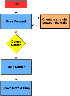
The concept program for the corridor competition is drawn in the following schematic:
To make this program possible, the system has a main loop with a case switch. This will activate the functions that are required at that moment. When for example the corner is detected it will switch to that function.
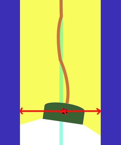
Driving Straight: To drive straight the robot measures the closest distance to each wall and also the corresponding angle. Using this information the orientation of the robot and the position in the corridor is determined. Using a controller, the robot will drive forward and correct its position until it is moving forward in the middle of the corridor.
Corner Detection: The corner is detected by looking at an angle of 90 degrees. If there is a sudden change in that distance (opening in the wall) the system will switch to the corner function.
Turn into Corner: After detecting the corner, it will drive while keeping the corner at the same distance. After this it will drive straight until the walls disappear and stop.
Week 4: September 23 - September 29
Test on the Robot
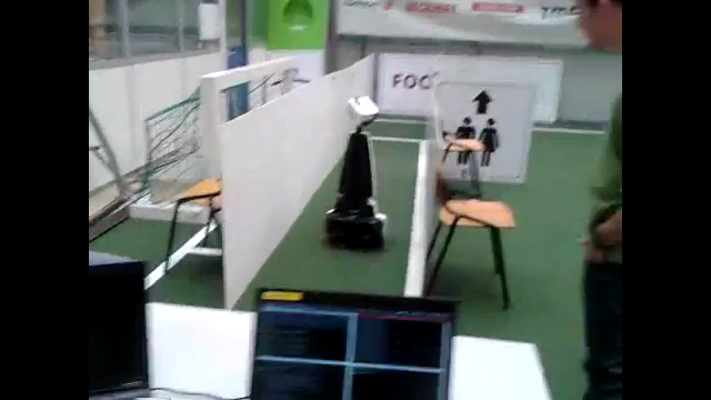
After we created a program for the Corridor Competition, the simulation showed good results. By running the program with the robot in various positions in the Corridor we concluded that the program was functioning properly. After that came the testing on the Robot. There were a lot of problems with the Robot. For that reason we were not able to have normal testing until one day before the contest.
In the end the tests on the robot were successful. The Robot was able to drive straight trough the corridor, however due to the hysteresis, friction and the low values on the controller it drove in a stretched S-shape, like a snake. The corner however was very smooth.
The Competition
After some problems where the robot would turn after initialization, the competition was a success in the second try. Group 9 set the third time of 4 groups what were able to finish the competition.
<br\>
Strategy
After the competition and a brainstorm session we came to the conclusion that this method is only effective for straight corridors with single exits. Watching the maze that is provided with the simulation is is clear that there are a lot of different types of situations. Also decisions on where to at certain junctions is not supported by the current code. Therefor the strategy should contain 'mapping'. This way there is a way to detect the path in front of the robot while also saving everthing that was discovered before. This should prevent driving into allready explored parts.
Week 5: September 30 - October 6
This week we started with a totally new design for the pico software architecture. For the corridor competition we only focused on a particular task, driving straight and take one corner. In the real maze more functions and software features will be required. We started by separating the existing code in even more individual functions. We split our group in 3 subgroups
- Frank and Filipe look into analyzing of the laser data and come up with a matrix of “edges” from which lines can be determined.
- Rens and Jeroen will use this information to determine a trajectory through the junctions based on “nodes”.
- Haico wil look into the arrow detection with the camera.
Finding 'Hard Points'
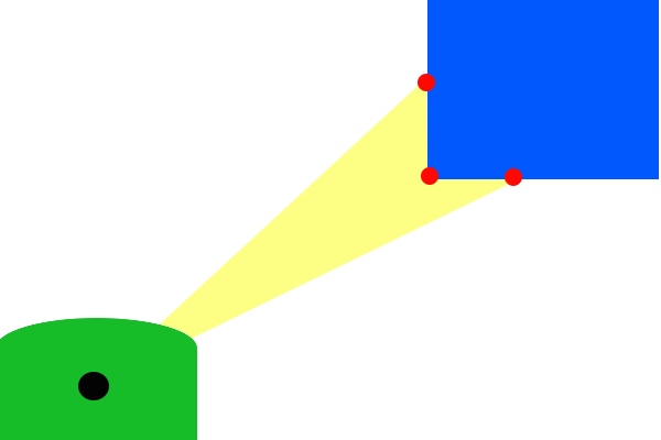
The way to find corners is based on scanning the entire range of the laser. From the position of the robot, a corner can be detected by finding a sudden change in the distance in another direction. Using this theory, there are 2 types of corners: one where the middle is closest and the distance grows from this point (a corner to turn around), and also a corner that is opposed to this (a corner to turn before). This way the robot and drive to a junction, determine the type, and then use this information to take the specific corner.
Determine Trajectory in Junctions
After the 'hard points' are known, the junction can be determined. This way we have the possibility to pick one of the directions and also drive trough it. Because there are only so many possible junctions, it is possible to prepare for all of these and determine the trajectory.
Vision
Haico looked for a solution.
Week 6: October 7 - October 13
- Determine junction type
Jeroen made a function in the c++ code to detect the type of junction when the robot is approaching one. How this has been done will be explained later.
- Arrow detection
Haico is still looking to detected arrows based on the camera data.
- Hough transformation for lines and edges
In the meantime Frank is working on the Hough transformation to detect lines and edges.
- Robot movement
Rens started with improving the way the robot turns around a corner and how to cross a cross section.
- Software architecture
Filipe has been looking on the final software architecture and stared with integrating individual functions.
- Testing on Pico
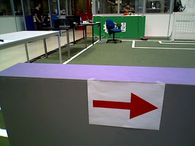
At the end of the week we booked some time on the actual robot to obtain some bag files of the camera. These bag files are used to test and tune the arrow detection algorithm. We placed an red arrow at the end of an corridor one time point to the left another time point to the right and during several drives through the corridor we recorded the camera footage.
Week 7: October 14 - October 20
- Wiki
We finally started with updating the wiki page of this group. In the PICO chapter we explain all the individual components of our software program. Jeroen will update the wiki when there is new relevant information available.
- Arrow detection
Haico finished together with Jeroen the arrow detection code to determine if we detected an arrow if it’s pointing to the left or right. This information is used in the “decision” function with the highest priority. How he designed the arrow detection will be explained later.
- Hough transformation for lines and edges
Last week Frank made a lot of progress with the Hough transformation he is able to determine lines and based on the intersections of lines he will determine edges.
- Robot movement
Rens finished the improvement of the way the robot turns around a corner and how to cross a cross section. He also made with Filipe the code for turning 180 degrees on the same spot. This is used when we are in a dead end. How we turn 90 or 180 degree is explained later. Filipe is looking into the controllers which we use to drive in the coners and try to optimize them more with PID based controllers.
- Software architecture
Each time we finish a separate function, for example this week the arrow detection function is finished, Filipe intergrades it in the final program.
- Functions and features
Jeroen wrote a software function which look when PICO is at a Cross, T_left or T_right junction if there is an arrow in front of PICO in a large distance than the current junction. If that is the case PICO will drive straight ahead instead of exploring the junction currently in front of PICO. Jeroen also made a function which is called when PICO wasn’t able to detect an junction based on the Hough transform data. When this occurs PICO will drive a few cm back and tries again to determine at which junction PICO is.
- Testing on Pico
During one of the final testing sessions on the pico we encountered some problems with the turning and driving straight functions. We assume that the controllers which we developed of this are not good enough to deal with the stick-slip which the robot has with the driving surface. In the simulations we were able to perfectly drive through a random maze but in reality we kept hitting the opposite wall when turning left or right. At the moment we were able to turn we were that much off-centered in the corridor the controller and the robot needed to much space to reposition itself that we did not arrive perfectly centered and straight for the next junction causing the junction detection to fail determining the correct junction. In the weekend we have to redesign these controller otherwise we will probably have same problems during the final competition.
Week 8: October 21 - October 27
PICO
Assignment
This course is about software design and how to apply this in the context of autonomous robots. The accompanying assignment is about applying this knowledge to a real-life robotics task in which ROS will be the standard software framework. The goal of the assignment is to get the real-time concepts in embedded software design operational.
The concrete task that has to be solved is to let the PICO robot find his way out of a maze. The final demonstration by each participating group of 4-5 students will be performed during a contest, the winner of which is the group that exits the maze in the shortest amount of time.
Some theory about solving mazes
We start with obtaining some general and basic methods of solving a maze. With these methods in mind we can perhaps determine a good solution for the maze competition in the embedded motion course.
- Follow the wall
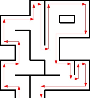
The name already explains what this methods does, it follows a wall. It is not very difficult to program this for the pico robot. At the initial point of the maze the robot just choses either the left or right wall and will follow this wall till it find an exit or when there is no exit it will return to the starting point. For the situation where the left wall has been chosen, when the robot is at a junction it always prefers to turn left or when this is not possible it goes straight ahead. There is no need to keep track of the junctions it took in the image below we depicted an example of this method.
In the image above we followed the left wall and as can be observed this is not the most efficient method however it will find an exit.
- Trémaux's algorithm
Trémaux's algorithm, invented by Charles Pierre Trémaux[1], is an efficient method to find the way out of a maze that requires drawing lines on the floor to mark a path, and is guaranteed to work for all mazes that have well-defined passages. A path is either unvisited, marked once or marked twice. Every time a direction is chosen it is marked by drawing a line on the floor (from junction to junction). In the beginning a random direction is chosen (if there is more than one). On arriving at a junction that has not been visited before (no other marks), pick a random direction (and mark the path). When arriving at a marked junction and if your current path is marked only once then turn around and walk back (and mark the path a second time). If this is not the case, pick the direction with the fewest marks (and mark it, as always). When you finally reach the solution, paths marked exactly once will indicate a direct way back to the start. If there is no exit, this method will take you back to the start where all paths are marked twice. In this case each path is walked down exactly twice, once in each direction. This method is more difficult to program as the follow the wall algorithm because we need to keep track on which turns we took and how many times we visited a corridor.
[1] Public conference, December 2, 2010 - by professor Jean Pelletier-Thibert in Academie de Macon (Burgundy - France) - (Abstract published in the Annals academic, March 2011 - ISSN: 0980-6032) Charles Tremaux (° 1859 - † 1882) Ecole Polytechnique of Paris (X:1876), french engineer of the telegraph
- Shortest path algorithm
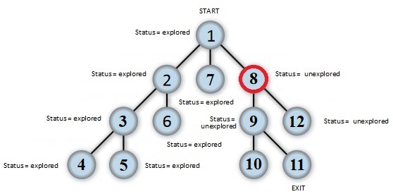
A way to solve a maze which for example contains multiple exits is a shortest path algorithm such as the Depth-first search. The general idea behind a Depth-first search algorithm is that we examine a starting node, say 1. Then we examine all the neighbors of 1, then we examine all the neighbor which we find from the neighbors of 1, and so on, until we reach the desired ending node or until we have no nodes to examine (in this case no path will exist). Naturally, we need to keep a track of all the nodes to assure that no node is processed more than once. This is accomplished by linking a field "status" with all the nodes. An example is shown below.
Again this method is more difficult to program as the follow the wall algorithm because we need to keep track on which node we visited.
A usefull website for more information about maze solve algorithms is: http://en.wikipedia.org/wiki/Maze_solving_algorithm
Software architecture
- ROS nodes
- C++ layout
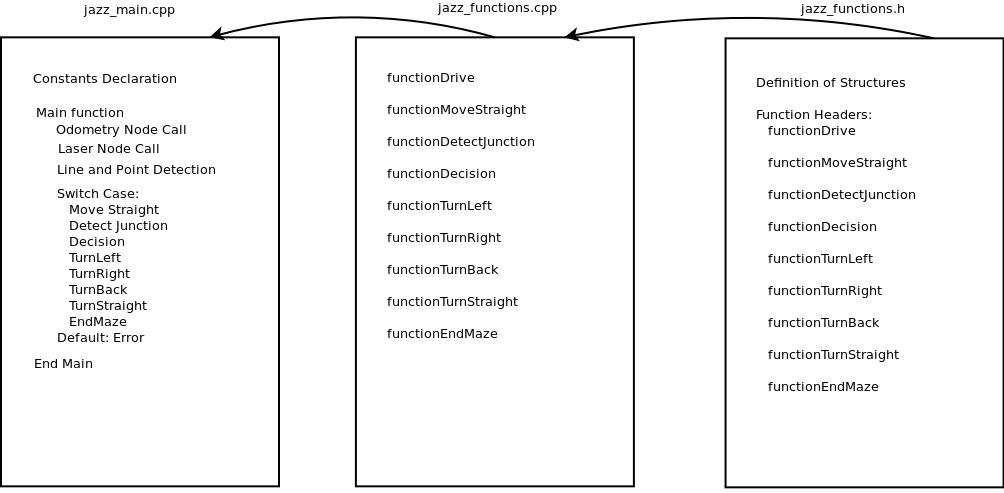
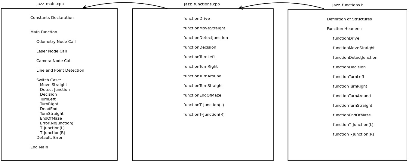
As shown above our cpp program is divided into 3 files. "jazz_main.cpp", "jazz_functions.cpp" and "jazz_functions.h". In "jazz_main.cpp" we define our global variables and constants. All our secondary functions will be called from the main function. This main function starts by calling the laser and odometry nodes. Then it starts a loop that goes through a line and point detection code. Further beggins a switch case statement where several cases are treated, each one is calling a secondary function from the file "jazz_functions.cpp". These cases can be observed in the flowchart above. The file "jazz_functions.cpp" is used as a support to place all necessary functions to the main function. In "jazz_functions.h" we declare our structures and headers of the functions used in "jazz_functions.cpp".
- Main program flow
The main program flow is depicted below.
Laser data interpretation and processing
- Data preprocessing
The original data coming from the laser is stored in the parameter 'Scan' where it is filled with 270 degrees of data with increments of 0.25. This means the array contains 1080 values that give the distance the wall. Experimentation showed that the robot also scans itself with this sensor so to get rid of this the first and last 5 degrees are removed (total of 40 values).
Also there is some noise in the data signal due to the environment and the sensitivity of the sensor, which has to be solved. The method used is to filter this data. The filter that is written for this data works as the following: it runs trough the entire laser data from the 20th to the 1060th value (cutting off the first and last 5 degrees). On every particular value its groups the 5 values on both sides (around 1 degree each side). It then sorts this set of values from low to high. The next step is to only take the middle 3 values (assuming they represent the correct angle) and average these. This value will be written into a new Dataset that is used in the rest of the program.
After the filter, the new Dataset is also used to determine the closest distance to the left of the Robot with the linked angle, and the same of the right side. This information is used to drive the robot trough corridors and around corners. The method used is to loop trough the data on both sides and find the lowest value and remember the angle.
Detecting points by applying Hough algorithm and Jumps in laser signal
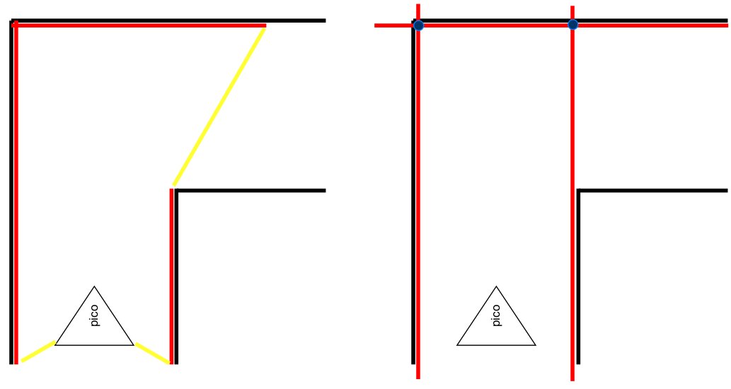
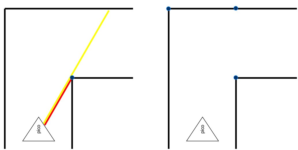
In order to navigate through the maze, points of interest have to be extracted out of the data coming from the laser sensor. Because the environment is constructed out of rectangular shapes, these points of interest resemble 90 degree corners. The following two methods are being used to obtain these points:
- One is by applying they hough transform on the laser data, which generates lines. By taking the intersection between these lines, points of interest are obtained. The left image here below shows what the laser data look like. The image to the right shows the lines obtained after applying the hough transform on the laser data. The intersection of the lines, shown in blue, are the points of interest.
- The other method being used, is by searching for large differences in distances between neighboring points in the laser data. These jumps in the signal are induced by lines of sight along corners. The left images below shows this situation.
Together these points give a distinct picture of every type of junction (T-, Cross- and L-junction, ) that can be encountered, shown in the right image above.
Some physical lines in the laser data are represented by two or more slightly different lines after applying the hough transform. Taking the intersection between these lines generate double points. When the 2-norm between two points are below some threshold, they are averaged to make one point out of them.
Junction detection
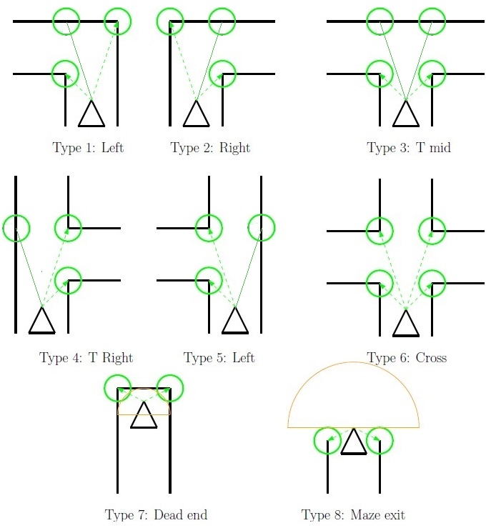
While driving through a corridor we keep searching for a gap on either the left side of the robot or the right side. This detection of gaps runs parallel while driving straight. At the moment we detect a gap we stop immediately and we start with the determination of the type of junction which we encountered. This is done based on the lines and edges data explained earlier. In the figure below we shown all type of junctions which our program can detect.
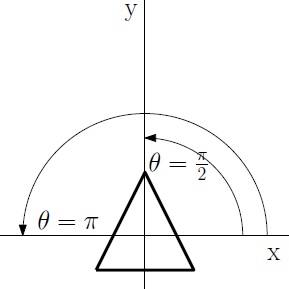
As can be observed with the green circles around the most dominant edges at a specific junction each type of junction as unique features. Based on these unique features we can determine what type of junction it is. For each time we summarize how we do this. To do that we first explain a bit how we see points on a map. We place a simple 2D grid on the center of Pico and use the standard convention of angles, meaning that an angle of 0 is a line parallel to the x axis on the right side of the robot. A line with angle of pi/2 is straight ahead etc. as shown in the figure below.
- Type 1 - Left: If we have two dominate edges and one edge is left side of the robot and one edge is on the right side and that the edge on the left side is closer that the one at the right side ( with certain margins of course) we determine it is a junction to the left.
- Type 2 - Right: The same as with left but then the otherway around. If we have two dominate edges and one edge is left side of the robot and one edge is on the right side and that the edge on the right side is closer that the one at the left side we determine it is a junction to the right.
- Type 3 - T_Mid: If we have two dominate edges where one edge is on the left and one edge is on the right side of the robot and they are approximately the same distance away from the center of the robot ( again with a certain margin ) and we don’t detect a wall in front of the robot we determine it is a T junction with left and right corners.
- Type 4 - T_Right: If we have two dominate edges and both of them are on the right side of the robot where one edge is further way as the other we determine it is a T junction where we can go straight ahead of right.
- Type 5 - T_Left: If we have two dominate edges and both of them are on the left side of the robot where one edge is further way as the other we determine it is a T junction where we can go straight ahead of left.
- Type 6 - Cross: If we have four dominate edges and two of them are on the left side and two on the right side we determine a cross section.
- Type 7 - Dead end: If we have two dominate edges where one edge is on the left and one edge is on the right side of the robot and they are approximately the same distance away from the center of the robot ( again with a certain margin ) and we detect a wall in front of the robot we determine it is a dead end.
- Type 8 - End of maze: If we have two dominate edges where one edge is on the left and one edge is on the right side of the robot and they are approximately the same distance away from the center of the robot and we don’t detect a wall nearby we found the exit of the maze.
Pico movement / driving
- Moving staight
- Turning left or right
- Crossing a cross
- Dead end
Arrow detection
The detection of the arrows will be done by detecting the extreme points of arrow, using OpenCV library. We used OpenCV library in our ROS environment. We will use a simple tutorial for test our Jazz Camera. This is given in the last class lesson. We implement the OpenCV library in our environment and start step by step our procedure.
- Step 1.) Convert RGB image to HSV image
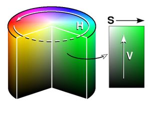
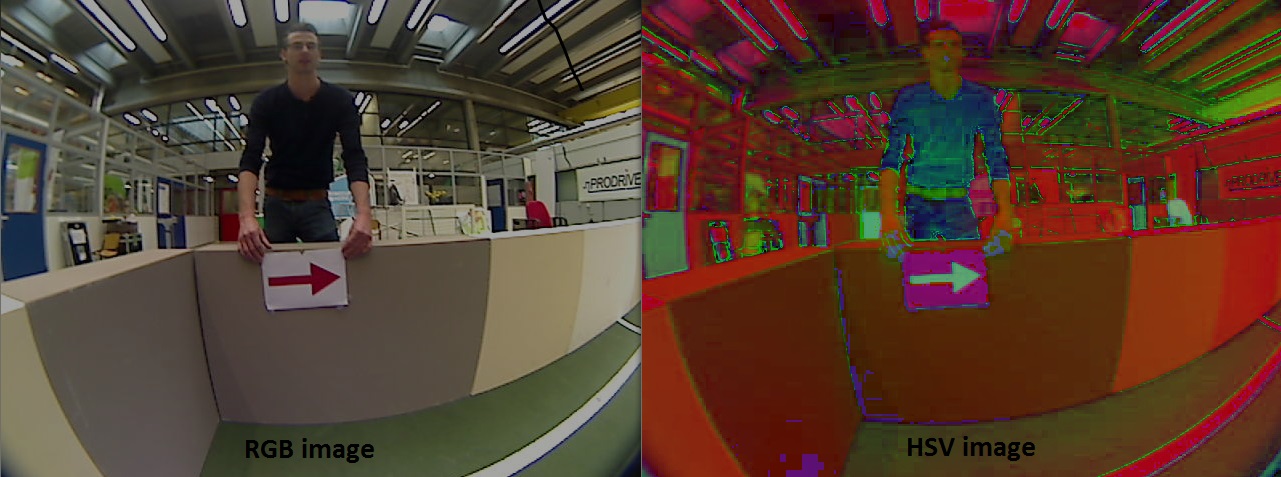
Our first step is to convert the RGB image to HSV[1]. HSV stands for hue, saturation, and value. It has values from 0 to 255 for each of the parameters. The colors begin with red, pass through yellow, green, cyan, blue, magenta, and return to red. The advance of using HSV is that you can use a color for different illuminations by using a hue and saturation value. A representation of the HSV model is shown in the figure below:
The figure below shows the convert image from RGB to HSV:
- Step 2 .) Threshold the HSV Image
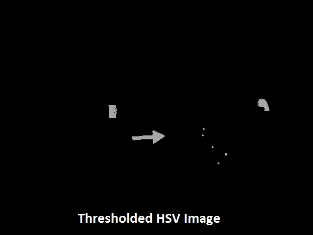
We used the HSV format so we can threshold the image. Because we are looking for a red arrow in our visualization picture. With threshold an HSV image we are sure that we are looking for a red object. With the saturation and value it is possible to be less sensitive to light. Some thresholds for the H, S and V parameters can be applied to the image, such that the pixels that have values in between these thresholds will be shown as white and the rest will be shown as black. The thresholds that are used are as follows:
- Minimum values: Hue= 145, Saturation=200 and Value=90.
- Maximum values: Hue=190, Saturation= 295 and Value=200.
With the threshold we make the picture binary. White is all the red objects (what’s thresholds by the min and max values) and black the other colors. Our threshold picture can you see below:
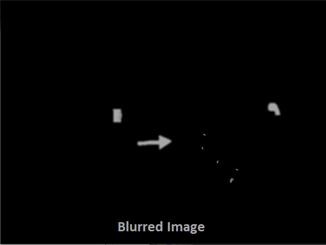
- Step 3.) Blur the Binary Image
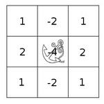
Smoothing, also called blurring, is a simple and frequently used image processing operation. We used blurring for eliminate noise in our object. So we eliminate noise in the contours. For our image we using the normalized box filter. It’s an OpenCV toolbox with the name “blur”[2] . The function smoothest an image using the kernel:
We used the parameters blurring kernel size=5. A kernel is essentially a fixed size array of numerical coefficients along with an anchor point in that array, which is located at the center. The picture below shows a kernel:
What this function does is as follow: Place the kernel on top of a determined pixel, with the rest of the kernel overlaying the corresponding local pixels in the image. Multiply the kernel coefficients by the corresponding image pixel values and sum the result. Place the result to the location of the anchor in the input image. Repeat the process for all pixels by scanning the kernel over the entire image.
The blurred image is shown in the figure below:
- Step 4.) Sharp image
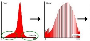
The next step is sharp the image again. So the contours of the objects will be sharper. For this we used Histogram Equalization[3]. It’s an OpenCV function called “equalizeHist”. It quantifies the number of pixels for each intensity value considered. It is a method that improves the contrast in an image, in order to stretch out the intensity range.
To make it clearer, from the image above, you can see that the pixels seem clustered around the middle of the available range of intensities. What Histogram Equalization does is to stretch out this range. Take a look at the figure below: The green circles indicate the underpopulated intensities. After applying the equalization, we get an histogram like the figure in the center. The resulting image is shown in the picture at right.
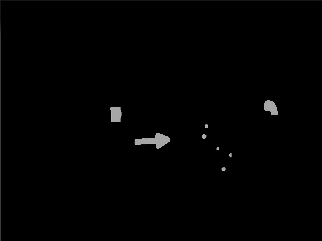
- Step 5.) Threshold again
We threshold again to a binary picture so it’s only a black and white with picture with a value for white = 255 and black = 0.
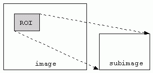
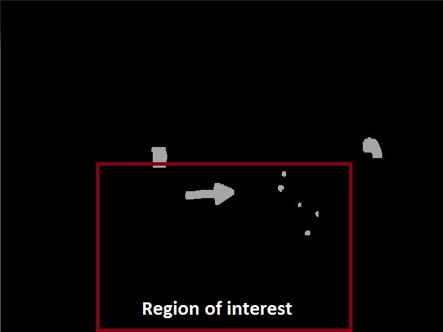
- Step 6.) Region of interest
We are only interested in objects in the maze so we want to eliminate the environment outside the maze. Because otherwise other big objects in the same color as the arrow can be gives some problems. So we eliminate the environment outside the maze with the OpenCV function myROI. We used rect MyRoi for select the rectangle view of the image we want.
In this figure can you see the region of interest of the Thresholded image:
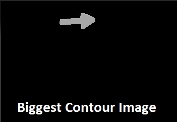
- Step 7.) Find biggest contours in the cropped image
After the conversion to a binary image and region of interest there was still some noise in our image. Probably as a result of reflection of the light and the presence of other red objects near the red arrow. Therefore we search in the binary image for closed contours, i.e. for object pixels that are connected with each other, using the FindContours function of OpenCV. For each contours we calculate the area and store the biggest contour. Since only the biggest contour remains the residual noise is filtered out and only a possible arrow is left. We used this[4] website for help. In the figure below shows the biggest contour:
- Step 8.) Calculate the extreme points
To recognize an arrow we want to now the location of the extreme points[5] of the arrow. Extreme Points means topmost, bottommost, rightmost, leftmost points of the object. The figure below shows you the extreme points of an arrow. The green dots are the extreme points.
I will explain the topmost extreme point. First we scan the picture: we start by the first row and scan every column for a white pixel (value 255). When we found a white pixel with value 255 we store the location X (row) and Y (column) as topmost. For bottommost we scan from bottom to top, leftmost from left to right and for rightmost we scan the picture from right to left for a white pixel.
- Step 7.) Calculate the centroid of the arrow
So the first step to recognize an arrow is calculating the centroid of the arrow. The red dot in the figure above shows the centroid. We calculated with two difference methods.
1.) Use the moment function of the OpenCV toolbox. An image moment[6] is a certain particular weighted average (moment[7]) of the image pixels' intensities. Central moments[8] are defined as:
Where centroid X =![]() and centroid Y =
and centroid Y = ![]() are the components of the centroid[9].
are the components of the centroid[9].
2.) We calculated the middle of the two extreme points on the right en left site of the arrow.
Centroid X = ( MostRight X – MostLeft X )/ 2 + MostLeft X
Centroid Y = ( MostRight Y – MostLeft Y )/ 2 + MostLeft Y
- Step 8.) Recognize the direction of the arrow.
We are only interested in an arrow to direction left or right. For this we used the extreme points MostUp and MostBottom. If the points MostUp and Mostbottom both on the left side of the centroid, the direction of the arrow is left . If the points MostUp and Mostbottom both on the right side of the centroid, the direction of the arrow is right. There is no arrow when the MostUp and MostBottom points both an difference sides of the centroid.
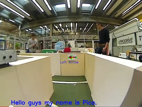
In the video below you can see the result of the arrow detection.
Maze solve algorithm
In this section we explain what kind of maze solve algorithm we used in the final contest. As mentioned above we investigated several methods of solving a maze on an efficient and fast way.
- Back-up program
To be sure that we at least find the exit in the maze we started with the constructing of a “simple” program were we follow either the left or right wall also known as the “follow the wall” algorithm as explained earlier. We will use this follow the wall method if we got lost in the maze and as backup if our more advanced maze solving algorithm fails to find an exit. For the follow the wall algorithm we drive Pico till an junction and turn always to the same direction if that is possible if we can’t drive in the preferred direction we drive straight ahead.
- Main program
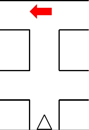
The main maze solve method which we are going to use during the final competition is somewhat based on the Depth-first search mentioned in the “Shortest path algorithm” mentioned earlier. When PICO drives towards an junction it stops there to analyze the type of junction in is facing this is done “Determine_junction” function. While the “Determine_junction” is running the robot stands still for a small time duration this is to improve the results of the Hough transformation and edge detection. This function then returns what kind of type of junction is facing how this is done is already explained in the Line and edge detection using Hough algorithm section. Based on this results we go either left or right at a corner to respectively the left or right side. If we detect an T_mid junction we also check if the Arrow_detection functions sees an arrow how this works is explained in the Arrow detection section. If it detects an arrow at the wall in front of PICO it goes to that direction of course. When we encounter an junction with multiple directions and we don’t find an arrow we will explore the most left directions first. We built a nice feature into the software of the robot. It will when we are at an Cross, T_Righ or an T_Left junction scan beyond that junction and look for an arrow in de far distance as displayed in the figure below for the cross junction.
When we detect an arrow in the far distance we ignore the current junction and just go straight ahead towards that arrow assuming of course that each arrow is pointing towards the exit.
When we detect an dead end we make a 180 degree turn and continou driving to unexplored terrain. Because of the priority of first exploring the left side at junctions we avoid that we drive towards the entrance of the maze instead of the exit. The end of the maze is detected by only two points and a large space in front and around the robot.
If for some reason we drive towards a dead end or when the junction detection function is not sure at what kind of junction the robot is, we drive a few cm back to rescan the junction again and hopefully obtain the proper data in the second try. If this fails again we stop the robot because we cant drive back to far without being sure we dont hit a wall.
