Embedded Motion Control 2013 Group 5: Difference between revisions
No edit summary |
No edit summary |
||
| Line 126: | Line 126: | ||
Our current software architecture can be seen in figure four. We have centralized our motion planning in the strategy node. This node receives messages from the /safe_drive node, which tells the system to either stop or continue with the operation (driving/solve maze). | Our current software architecture can be seen in figure four. We have centralized our motion planning in the strategy node. This node receives messages from the /safe_drive node, which tells the system to either stop or continue with the operation (driving/solve maze). | ||
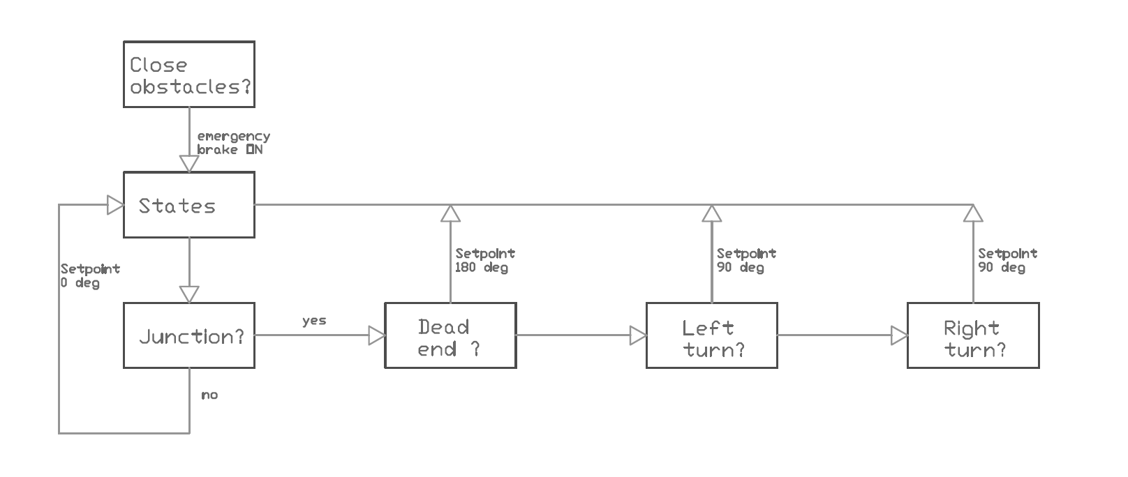
If the safety is off, the /strategy node starts computing the next step. If it is on, pico is halted until resetted. | If the safety is off, the /strategy node starts computing the next step. If it is on, pico is halted until resetted. The decisions made in these steps can be visualized as followed: | ||
[[File:Steps.png|thumb|400px| Steps for driving]] | |||
Next, the data gathered from the laser range finder (LRF) is converted into a set of lines using the hough transform. Here, each line is represented by a radius (perpendicular to the line) and an angle w.r.t. reference line. The top view of the robot with these parameters are depicted in figure XXX_show. | Next, the data gathered from the laser range finder (LRF) is converted into a set of lines using the hough transform. Here, each line is represented by a radius (perpendicular to the line) and an angle w.r.t. reference line. The top view of the robot with these parameters are depicted in figure XXX_show. | ||
[[File:Coor.png|thumb|400px| Agreed coordinate system for PICO]] | |||
Using these angles, we can identify the walls that are located to the left and to the right of PICO by sorting the data received from the hough transform by angle. We now know the location and orientation of the left and right wall w.r.t. PICO. | Using these angles, we can identify the walls that are located to the left and to the right of PICO by sorting the data received from the hough transform by angle. We now know the location and orientation of the left and right wall w.r.t. PICO. | ||
| Line 176: | Line 178: | ||
Before we transform the LRF data using the Hough function, we check at which type of surroundings we are dealing with. There are a number of possibilities, which are displayed in the figure below. | Before we transform the LRF data using the Hough function, we check at which type of surroundings we are dealing with. There are a number of possibilities, which are displayed in the figure below. | ||
[[File:junctions2.png]] | [[File:junctions2.png|thumb|400px| Different types of junctions]] | ||
Using the laser range data, we can distinguish these situations by analyzing their values. Each situation has an unique amplitude-angle characteristic. We can generalize variations on the situations by assuming that a junction exit will reach a scanning range value above r_max. Setting the limit at r_max and thus truncating the scanning values will return characteristic images for each junction type: | Using the laser range data, we can distinguish these situations by analyzing their values. Each situation has an unique amplitude-angle characteristic. We can generalize variations on the situations by assuming that a junction exit will reach a scanning range value above r_max. Setting the limit at r_max and thus truncating the scanning values will return characteristic images for each junction type: | ||
Revision as of 22:25, 6 October 2013
Group members
| Name: | Student ID: |
| Arjen Hamers | 0792836 |
| Erwin Hoogers | 0714950 |
| Ties Janssen | 0607344 |
| Tim Verdonschot | 0715838 |
| Rob Zwitserlood | 0654389 |
Tutor:
Sjoerd van den Dries
Planning
| DATE | TIME | PLACE | WHAT |
| September, 16th | 15:30 | GEM-N 1.15 | Meeting |
| September, 23th | 10:00 | [unknown] | Test on Pico |
| September, 25th | 10:45 | GEM-Z 3A08 | Corridor competition |
| October, 23th | 10:45 | GEM-Z 3A08 | Final competition |
To do list
| DATE | WHO | WHAT |
| asap | Tim, Erwin | Exit detection |
| asap | Rob, Ties, Arjen | Move through the corridor |
Logbook
Week 1
- Installed the following software:
- Ubuntu
- ROS
- SVN
- Eclipse
- Gazebo
Week 2
- Did tutorials for ROS and the Jazz simulator.
- Get familiar to 'safe_drive.cpp' and use this as base for our program.
Week 3
- Played with the Pico in the Jazz simulator by adding code to safe_drive.cpp.
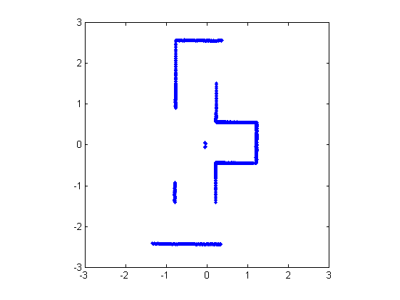
- Translated the laser data to a 2d plot (see Figure 1).
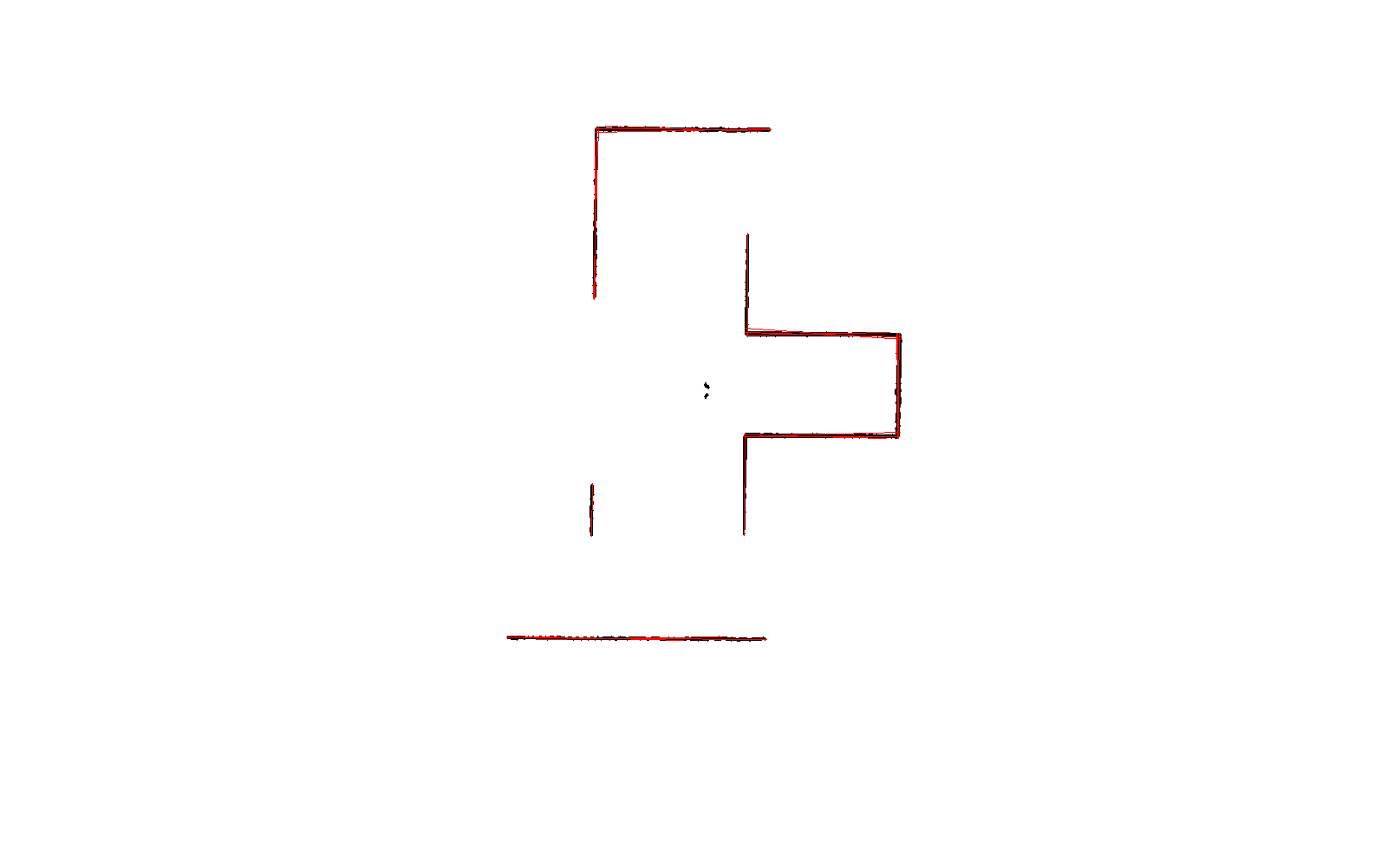
- Used the Hough transform to detect lines in the laser data. For the best result, the following steps are used:
- Made an image of the laser data points.
- Converted the RGB-image to grayscale.
- Used a binary morphological operator to connect data points which are close to each other. This makes it easier to detect lines.
- Detected lines using the Hough transform.
- To implement this algorithm in C++ code OpenCV will be used.
- The algorithm is implemented in the safe_drive.cpp.
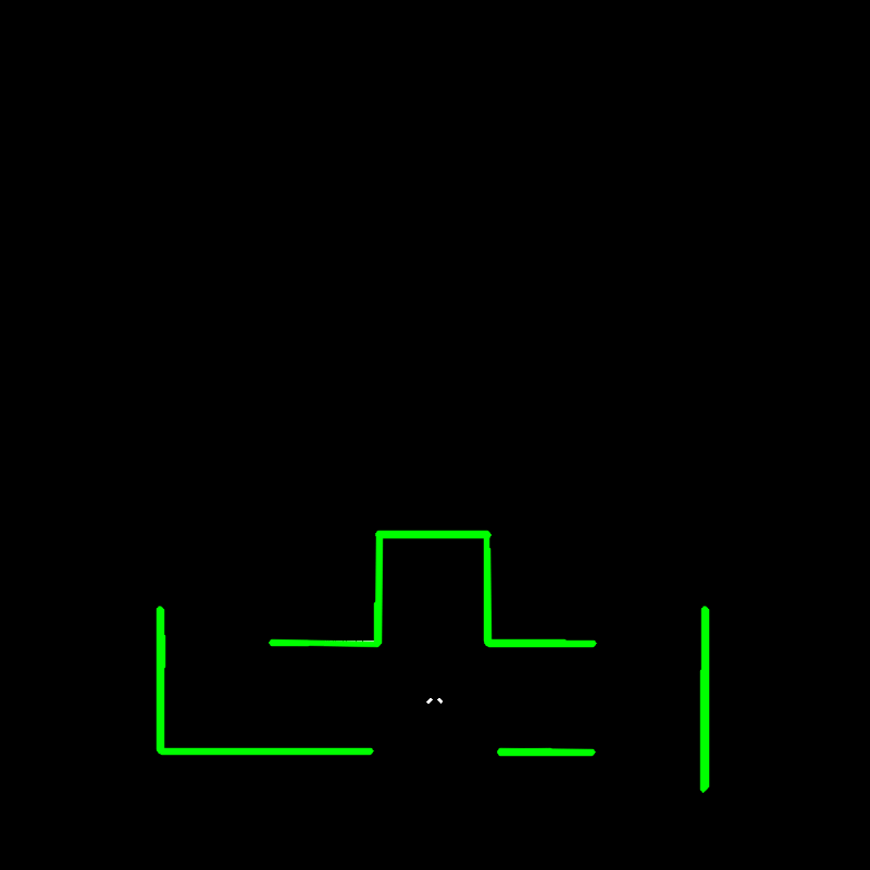
- The line detection method mentioned above works fine and is tested in the simulation (see figure 3,the green lines are the detected lines).
Week 4
- During the corridor competition pico failed to leave the maze, this was due to a paramount safety check (close range / collision) in the code. With no time left to edit, we were forced to give up. After this we decided to reorganize our software architecture by means of building seperate communicating nodes. This new scheme is depicted in figure four.
Software architecture
Our current software architecture can be seen in figure four. We have centralized our motion planning in the strategy node. This node receives messages from the /safe_drive node, which tells the system to either stop or continue with the operation (driving/solve maze). If the safety is off, the /strategy node starts computing the next step. If it is on, pico is halted until resetted. The decisions made in these steps can be visualized as followed:
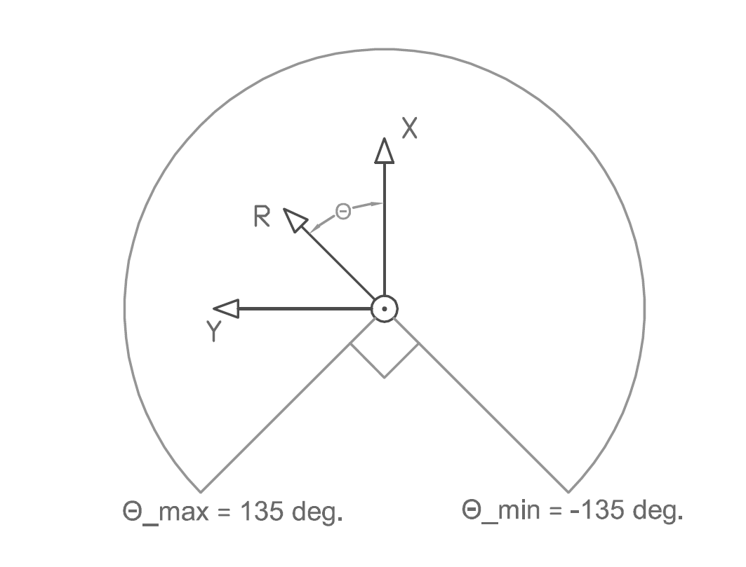
Next, the data gathered from the laser range finder (LRF) is converted into a set of lines using the hough transform. Here, each line is represented by a radius (perpendicular to the line) and an angle w.r.t. reference line. The top view of the robot with these parameters are depicted in figure XXX_show.
Using these angles, we can identify the walls that are located to the left and to the right of PICO by sorting the data received from the hough transform by angle. We now know the location and orientation of the left and right wall w.r.t. PICO.
Reference generator
The reference generator which is part of the strategy node, generates a reference point based on the surrounding walls.
Input: Vector of Walls (Nx1) (Structure Wall consists of - d: distance to wall - theta: angle between line perpendicular to wall and x-axis of Pico)
Output: Reference point in the corridor
Algorithm:
1) Sort vector of Walls such that theta1<theta2<...<thetaN
2) Select the first entry of vector as right wall and last entry of vector as left wall.
3) Define a fixed frame (x0,y0,z0) on the left wall. x0 at left wall pointed in driving direction, y0 perpedicular to wall, pointed inwards to Pico, z0 along right hand rule.
4) Define position Pico (p1) in (x0,y0,z0) coordinates
5) Define angle Pico in (x0,y0,z0) coordinates
6) Define reference point (p2) in (x0,y0,z0) coordinates
7) Definieer referenceangle phi from (p1) t0 (p2) in (x0,y0,z0) coordinates
Assumptions:
1) Pico starts with his “face” pointed inside the corridor.
2) The referencepoint (p2) is positioned at the middle of the corridor, 1 meter ahead of Pico’s current position.
Example:
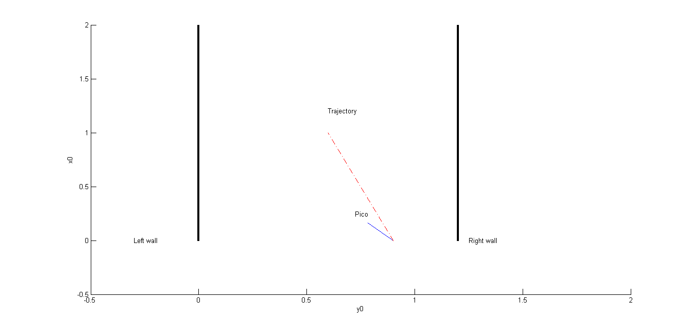
Figure 5 is an example of a situation of Pico in the corricor. The current position (p1) of Pico is the intersection between the blue and red line. The orientation of Pico is displayed by the blue line. The red line connents the current position (p1) with the reference point (p2). The error angle, which is given by the difference between the current angle of Pico and the reference angle. This error angle is used as controlinput fot the velocity of Pico.
Since our last meeting we have made some new tactics, which have yet to be worked out.
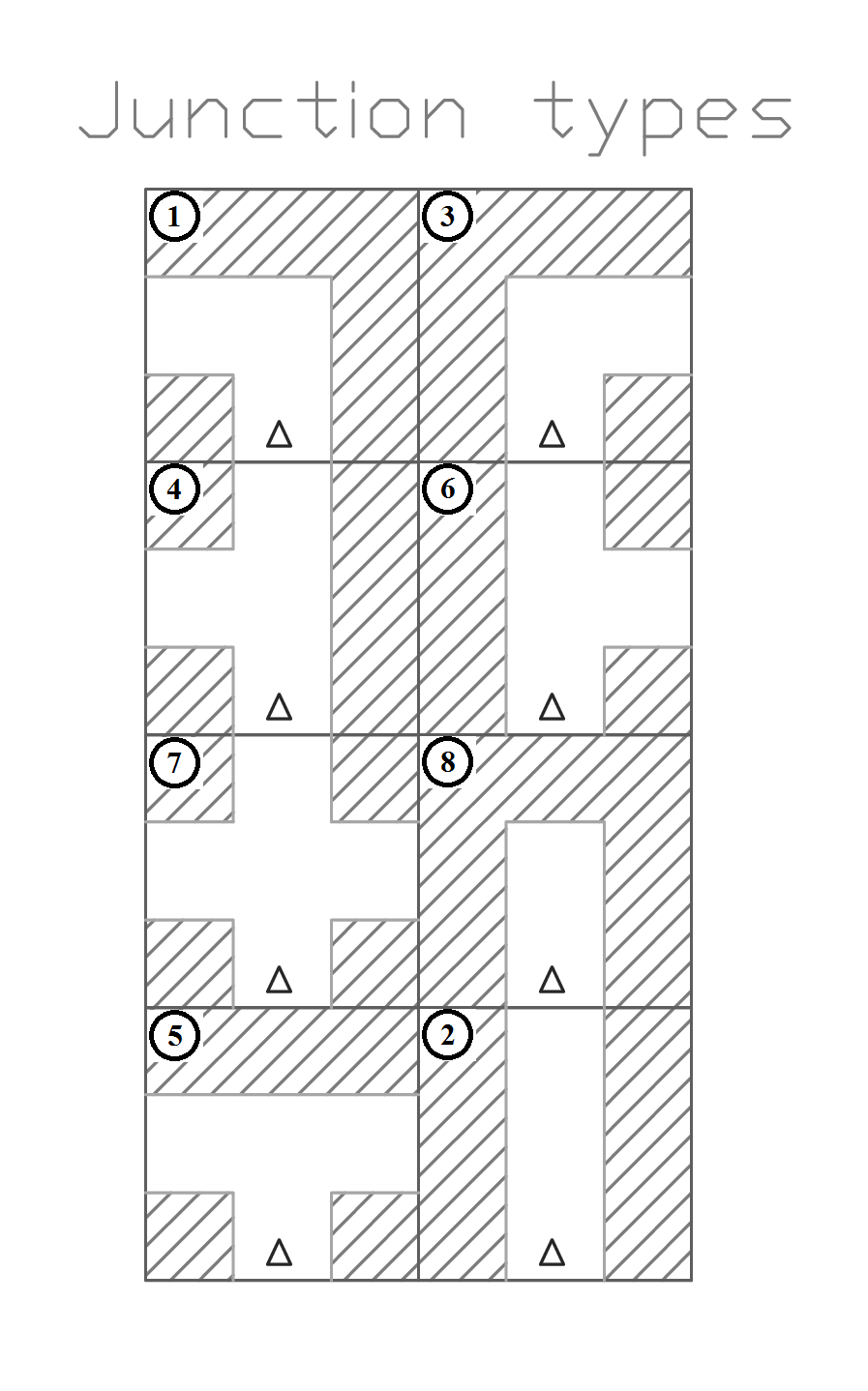
Before we transform the LRF data using the Hough function, we check at which type of surroundings we are dealing with. There are a number of possibilities, which are displayed in the figure below.
Using the laser range data, we can distinguish these situations by analyzing their values. Each situation has an unique amplitude-angle characteristic. We can generalize variations on the situations by assuming that a junction exit will reach a scanning range value above r_max. Setting the limit at r_max and thus truncating the scanning values will return characteristic images for each junction type:
figure t-splitsing/tim
If the average value (angle) of the truncated tops reach setpoint values (i.e. 0, 90, 180 degrees) w.r.t. the y axis we know what kind of junction we are dealing with. Now that we can identify the type of surroundings, we can tell if we have to navigate in a straight manner (corridor) or if we need to navigate towards an exit. With this information we can send messages to our motion node.
Up till now we have only used local positioning of PICO. No global mapping algorithm was implemented. This can be done by projecting maps on top of each other and aligning these with waypoints or markers. Since we are dealing with slip we have to add margins to these waypoints (e.g. circles) because the waypoints will not align exactly. An idea is to use a map without physical dimensions. This can best be represented by a tree structure, where the bottom of the tree is the starting point of the maze and the exit is in one of the branches. If we keep track of the junction types and orientation where we have been (where the branches split), we can rule out the investigated branches in the next run. The investigated branches can be identified by storing the spot and orientation of the junction by means of a "compass". Although simple in nature (just storing the junctions, orientation, location and wheter or not they have been chcked), it is hard to identify loops (If there are multiple ways (corridors) to reach the same junction). With no anti-loop mechanism they will be viewed as a new branch of possible solutions. If this is an actual problem, global mapping / localisation is required.
Some interesting reading
- A. Alempijevic. High-speed feature extraction in sensor coordinates for laser rangefinders. In Proceedings of the 2004 Australasian Conference on Robotics and Automation, 2004.
- J. Diaz, A. Stoytchev, and R. Arkin. Exploring unknown structured environments. In Proc. of the Fourteenth International Florida Artificial Intelligence Research Society Conference (FLAIRS-2001), Florida, 2001.
- B. Giesler, R. Graf, R. Dillmann and C. F. R. Weiman (1998). Fast mapping using the log-Hough transformation. Intelligent Robots and Systems, 1998.
- Laser Based Corridor Detection for Reactive Navigation, Johan Larsson, Mathias Broxvall, Alessandro Saffiotti http://aass.oru.se/~mbl/publications/ir08.pdf
