Embedded Motion Control 2012 Group 2

Group Members

Name	ID number	e-mail
T.H.A. Dautzenberg	0657673	T.H.A. Dautzenberg
V.J.M. Holten	0655090	V.J.M. Holten
D.H.J.M. v.d. Hoogen	0662522	D.H.J.M. v.d. Hoogen
B. Sleegers	0658013	B. Sleegers
		Mail to all

Tutor: Janno Lunenburg

Project Progress

Week 1

• Installation of Ubuntu, ROS and Eclipse
• C++ tutorial

Week 2

• ROS tutorial
• Meeting 1 with tutor
• Read Chapter 1 and 4 of Real-Time Concepts for Embedded Systems
• Made a presentation of Ch. 4 for lecture 2 [Slides]
• Prepared the lecture about Ch. 4

Week 3

• ROS tutorials continued
• Looking up useful information and possible packages on the ros website
• Formulating an idea to tackle the problem
• Trying to run and create new packages but running into some problems
• Presented Ch. 4
• Extra research regarding the API and Linux scheduler, as requested by Molengraft

Week 4

• Created a node which makes sure Jazz doesn't collide with the walls
• Created a node which enables Jazz to make the first left corner
• Research on different maze solving algorithm's
• Presented extra research regarding the API and the Linux scheduler briefly

Week 5

• Trying to create the path detection and autonomously cornering
• Made a start regarding arrow detection (strategy follows)

Week 6

• Further work on arrow detection
• Created a program with which we are able to accomplish the corridor competition
• First test with Jazz, Thursday 13:00 - 14:00
• The test turned out very well. We first had to rewrite some things in order to take the larger laser data array into account (1081 points instead of a lot less). But when this was fixed our first test immediately had the hoped result. The corner was detected and the robot drove through the corner properly without bumping into any walls. A link in the movies section was added where the result of a test is shown.

Week 7

• Corridor competition! Unfortunately Pico didn't succeed. At the first run the gain for the center drive controller wasn't tuned well resulting in an emergency stop. At the second run Pico drove quite well through the center of the corridor. Furthermore the left corner was detected and Pico drove to the setpoint correctly. Then the problem occured, Pico didn't turn enough which resulted in another emergency stop.

Week 8

• Making arrow recognition more robust
• First test

Week 9

• Second test
• Corrected several mistakes encountered during the test

Week 10

• Third and final test
• Made presentation

Components

• Wall detection
  • Laser scan data
• Arrow detection
  • Camera data
• Path detection (openings in wall and possible driving directions)
  • Laser scan data
• Control center (handels data provided by nodes above and determines the commands sent to the Jazz robot)

Software Design

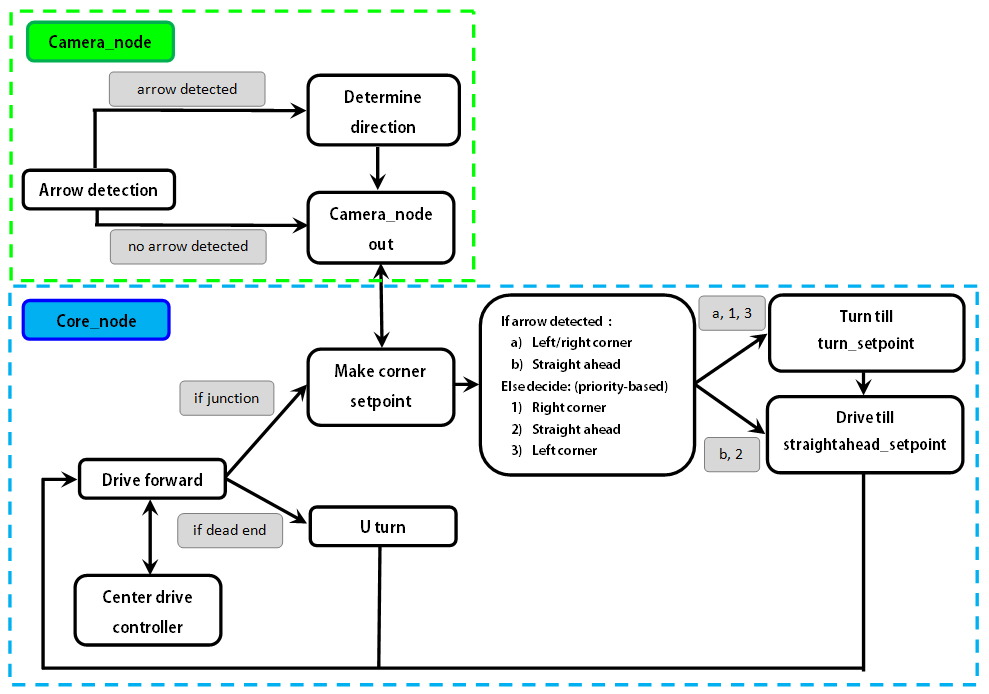
The software design is based on two nodes: one for arrow recognition and one Core node for all other operations. The camera node processes the images from the camera and will send 'left', 'right' or 'no arrow detected' over a topic. The Core node listens to the topics 'scan', 'odom', and the topic from the camera node. Publishing is done over the 'cmd_vel' topic. To maintain structure within the node, several structures and classes are used:

Structures

• Laserdata: a structure housing all information that is needed from the laser data provided by the robot. This also includes some data that has been manipulated.
• Odomdata: odometry data is stored in this structure as x- and y-position and the rotation around the z-vector.
• Corner: This struct contains parameters (mainly boolean) used in the discretization of making a corner over several stages that are identified during this process.
• Cornerdata: a variable of this type is used to store information needed in corner detection.

Classes

• Laser: this class contains functions needed to process the laser data from the robot. Upon extraction, the data is immediately manipulated i.e. relative x- and y-distances are computed using the range and the angle w.r.t. the robot and a number of minimum values from specific ranges are extracted from the data. A public function can be used to return a pointer to the instance of the structure 'Laserdata' where all the information is stored.
• Odometry: the basic functionality is analogous to the Laser class. The only manipulation of the data is done upon calculation of the angle (is provided in quaternions).
• Motion: A public function can be used to send movement commands. This function has the forward velocity and the angular velocity as inputs. Also, a check is conducted that will limit both velocities to a predetermined maximum value.
• Drive: This class is used to group the functions for the driving algorithm. Here, a drive command can be given by using a function where a distance can be entered that should be traveled in a forward direction. Contained in this class is a function to make a setpoint and a function that returns a boolean that is used to 'keep driving' as long as the setpoint has not yet been reached.
• Turn: Equal to the Drive class, this class is used to make a setpoint for an angular motion and to check whether this setpoint is already reached.

Apart from the classes, functions are used for corner detection and for the centering whilst driving through a corridor.

The 'main' loop is where the real program runs. It starts with the declaration of variables and a few initialization commands of ROSS. Hereafter, the subscribers and publishers are assigned their respective topics. A while loop is used to run the node in combination with the condition 'ros::ok()', a rate definition of the form 'ros::Rate', and 'ros::SpinOnce()' to refresh the subscribers and publishers.

Strategy

• Use the laser pointing forward to detect dead-ends, then turn 180 degrees.
• Use lasers pointing left & right to keep the robot in the middle of the path.
• Use lasers pointing 45 degrees left and right to detect corners. If there is a 'jump' in the data, there is a corner. The new and old laserdata are then used to create a setpoint in the middle of the corner to which it will drive. It will then turn left/right 90 degrees and start driving again until it detects a new corner.
• Use 2 nodes. One for the camera (which is only partly done) and the other node for the rest (corner detection, decision making, etc.). This is because the arrow detection should run at a much lower frequency due to the large amount of data.
• We use the right turn algorithm.
  • A right turn (if possible) is preferred above going straight ahead (if possible), and going straight ahead (if possible) is preferred above going left (if possible).
  • It is certainly not the most efficient technique, but relatively easy to implement.
  • A problem that might occur with this algorithm is that the robot will be circling around an 'island' for infinite time and never find the exit when his start position is at this 'island'.
    • Possible solution: The Pledge algorithm. The Pledge algorithm requires an arbitrarily chosen direction to go toward. When an obstacle is met, the right hand is kept along the obstacle while the angles turned are counted. When the solver is facing the original direction again, and the angular sum of the turns made is 0, the solver leaves the obstacle and continues moving in its original direction. The hand is removed from the wall when both 'sum of turns made' and 'current heading' are at zero. This allows the algorithm to avoid traps like starting at an 'island'. Note that this algorithm will not work when the robot has to find the way from an entrance on the outside of the maze to some goal within it.
    • When we heard we will start outside of the maze and have to find an exit outside of the maze we decided to halt implementing the Pledge algorithm. Since the denoted problem can not occur in this setting. The right turn algorithm will be safe.

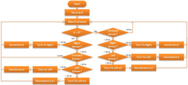
Path detection and corner setpoint creation

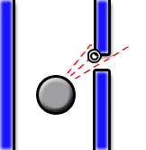
Robustness in laser detection

In order to make the software robust against holes in the wall or things like this, a small fan of laser points is used. While testing the robot detected a corner at a location where this really wasn’t possible, the reason turned out to be a small gap between the plates of the maze. So instead of basing the corner detection and path centering algorithms on a single point of the laser array, a number of points are now used. For the algorithms that determine the corner detection and the centering of the robot in the corridor, specific angles in the array of laser data points are used. Around this angle, we now use a series of points and determine the minimum of this series. This point is then used as before as the distance at that angle. In the picture below, this is the marked point. The series will consist of 15 points for a specific angle, which for a total of 1081 data points around 270 degrees, comes down to a fan of about 3 degrees. So when the corridor has a diameter of 1m, the robot can handle a gap of up to about 3cm.

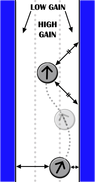
Center drive controller

For driving in the center there are 2 modes in which PICO operates: "near-wall" and "middle".

Near-wall

PICO will determine the distance perpendicular to the wall by selecting the minimum value of a range of lasers left and right. It will then turn left of right.

Middle

When it is near the middle of the corridor, Pico will use laserrange data front-right and rear-right of itself to align itself to the wall.

Arrow detection

Arrow recognition

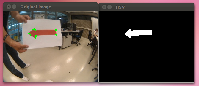
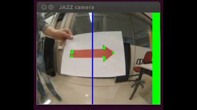
Left the original image with detected green dots, right the HSV thresholded image. We still have to figure out how to convert these green dots to whether or not the arrow is pointing left or right. (edit: this is no longer true) (we're also using the 2.x API (cv::Mat) instead of OpenCV 1.x API (CvArr))

Arrow recognition algorithm

Here the algorithm that is used to recognize the red arrow and its direction is described.

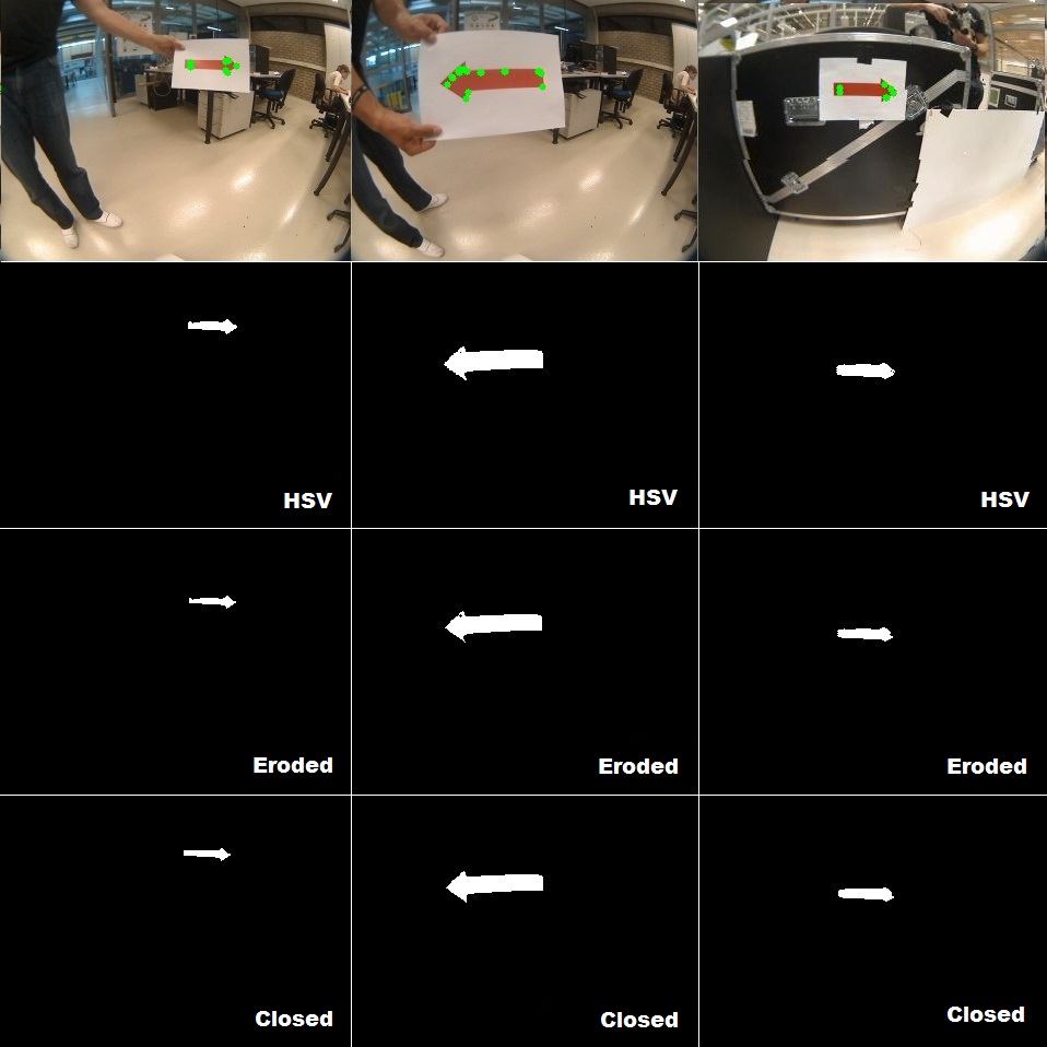
HSV

First the image is split up into its hsv values. This way the colors of the image can be easily distinguished. The HSV format is a common cylindrical representation of the Red/Green/Blue color model, it has values from 0 to 255 for each of the parameters. HSV stands for Hue (the color), Saturation (~amount of color) and Value (bright/darkness), which together make up the parameters for the color of a pixel. A representation of the HSV model is shown in the figure below.

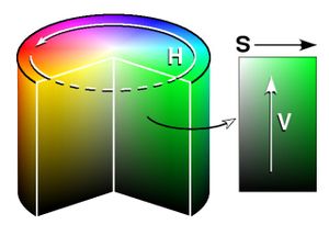
Some thresholds for the H, S and V parameters can be applied to the image, such that the pixels that have values inbetween these thresholds will be shown as white and the rest will be shown as red. The values of these thresholds are tuned to only let through the red of the arrow, such that the arrow can be destinguished. In the large image below, this is the HSV image (second from above). The thresholds that are used are as follows:

• Hue low: 111 - Hue high: 116
• Sat low: 123 - Sat high: 255
• Val low: 140 - Val high: 210

Erosion

The HSV image is then eroded to remove any noise from the image. What it does is to remove surfaces that are not connected to other surfaces. So it will remove small surfaces from the image and it will take away part of the edge of a larger shape. So the downside of this erosion is that we will "eat away" a little from the arrow. However any small dots or small surfaces that are not a part of the arrow will be removed. A cross erosion element of 3x3 pixels is used. The arrow after the erosion is shown in the large image below.

Closing

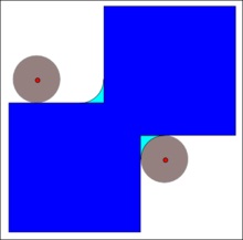
The eroded image is then "closed". This means that we attempt to close any gaps inside the image. So what is does to the eroded image of the arrow is to close any holes in the arrow and also it fills the outsides of the arrow a little. So it also removes some of the damage that the erosion might have done to the arrow itself. A Rectangular closing element of 12x12 pixels is used. The rectangular shape was chosen because it will theoretically not remove the edges and shape of the arrow as much. A circle element might for instance blur an edge of the arrow. In the closing figure below, the way in which closing works is shown for a circle element. The arrow after the closing is shown in the large image below.

Corner Detection

The function goodfeaturestotrack is then performed on the closed image, here the algorithm finds the corners of the image and saves their locations. In the large image below, circles are drawn at the positions of the found edges so we can see where they are located. These corners are used to see to what side the arrow points.

Arrow & Direction detection

So up till now we have an algorithm that first finds only a specific color and blocks out the rest of the image. That image is then eroded and closed in order to remove any noise. After that corners are detected on it, and these corners can now be used. However, first we need to know that pico is looking at an arrow. This arrow detection is done by first eroding the HSV image very heavily. This means that only very large areas in the camera will still be present in the image after the erosion. So if the arrow would be far away for instance, then the image would return black. Then we use the function goodfeaturestotrack to draw corners onto the image, if however the image is completely black, no corners can be drawn. So if the amount of corners detected is zero, we know that we are not looking at an arrow. These steps for detecting if we are looking at an arrow are implemented before the other processing steps in order to not do unnecessary computations when we aren't looking at an arrow. So say we now detect that we are looking at an arrow and the corners of the arrow are drawn on the closed image. We first calculate the mean of the x value of the corners, this means that we try to find the center of the arrow, here we draw a vertical line. Then we use two separate properties of an arrow to see to what side the arrow is pointing. First, we sum up the amount of corners left of the center (the vertical line) and right of the center. We know that due to the shape of an arrow, we should theoretically have more corners on the side where the arrow is pointing than on the other side. So if the amount of corners to the right is larger than to the left, this algorithm gives out right. Second, we look for the maximum and minimum y value on either side of the center and calculate the difference per side. We know that the side to which the arrow is pointing should have a larger maximum vertical distance than the other side. So if this distance is larger to the right than to the left this algorithm gives out right. Now these two algorithms are compared, and whenever they agree on a side we know that the arrow is quite certainly pointing in that direction. To incorporate for any noise or other problems, we make pico only respond to the notion of the camera whenever the functions agree for a few times in a row (so 2 or 3 times right, for instance).

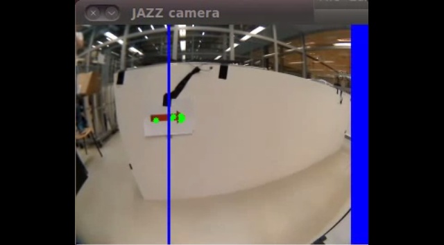
In the clips below you can observe this detection method in practice on the robot, here the side that the robot gives out is denoted by the green bar on a certain side.

Movies

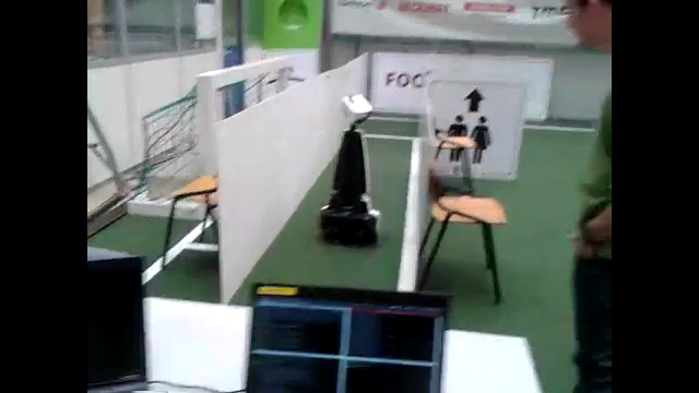
Corridor competition test

<br\>

Arrow recognition (with the given bag file)

<br\>

Arrow recognition (more robust algorithm and with our own bag file)

<br\>

2nd Maze test

<br\>

2nd Maze test with corner correction

<br\>

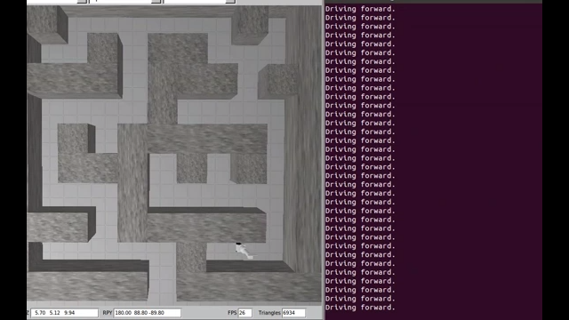
Maze completion in simulator

<br\>

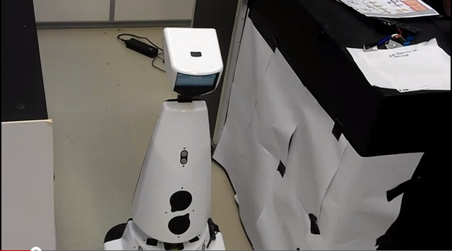
Final test with real robot

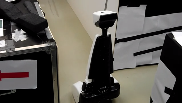
Live maze test<br\>

Presentation of group 2

Possible improvements

In this section we present future recommendations, which we were not able to implement anymore.

Arrow detection

• Convert the image to HSV.
• Use the "k-means algorithm" to cluster nearby objects.
• Use "connected compenents labelling" to find the different objects.
• Use "region filling" to fill in any gaps due to lightning.
• Calculate the inertia/covariance matrices for each object and find its eigenvalues and eigenvectors.
• Divide both eigenvalues of each object and extract the arrow which is the object with the same heigth/width ratio as the arrow. The largest eigenvalue is longitudinal with the arrow.
• Make a line move perpendicalur over the corresponding eigenvector. Where the line is maximal, is where the head of the arrow is.

This way the direction of the arrow can be detected more robustly than the algorithm we used. This can also detect if the arrow is pointing in the drive straight arrow direction.

...

• ...