PRE2016 2 Groep1: Difference between revisions
No edit summary |
No edit summary |
||
| (122 intermediate revisions by 4 users not shown) | |||
| Line 8: | Line 8: | ||
'''PRE2016 Q2 Group 1 - Main page''' | '''PRE2016 Q2 Group 1 - Main page''' | ||
</h1> | </h1> | ||
<div style="position:relative; top:.25em; font-size:100%">'''<br/>Koen Damen - 0893034<br/> Stijn de Milliano - 0816573<br/> Ralf Reinartz - 0892456<br/> Zjeraar Scharis - 0651925<br/> Stefan Thijssen - 0888708 | <div style="position:relative; top:.25em; font-size:100%">'''<br/>Koen Damen - 0893034<br/> Stijn de Milliano - 0816573<br/> Ralf Reinartz - 0892456<br/> Zjeraar Scharis - 0651925<br/> Stefan Thijssen - 0888708<br/> '''</div> | ||
| rowspan="32" width="10px" | | | rowspan="32" width="10px" | | ||
| rowspan="32" width="5px" | | | rowspan="32" width="5px" | | ||
| Line 17: | Line 17: | ||
|} | |} | ||
<br/> | <br/> | ||
{| cellpadding="10" | {| cellpadding="10" | ||
|-valign="top" | |-valign="top" | ||
|width="49%" style="border:2px solid #2E9AFE;text-align: justify;background-color:white"| | |width="49%" style="border:2px solid #2E9AFE;text-align: justify;background-color:white"| | ||
<h1 style="font-size:180%; border:none; margin:0; padding:0"> | <h1 style="font-size:180%; border:none; margin:0; padding:0"> | ||
'''Welcome''' | '''Welcome''' | ||
</h1><br/>Welcome to the Wiki of the first and only group of Project Robots Everywhere 2016 Quarter 2. On this page we will keep track of our progress during the project, this way everybody can see the progress we are making and we can organize the information we have gathered. Feel free to take a look around. We have divided our progress into the separate weeks we worked on the project explaining for each week what we did, what results we got and what we plan to do with those results. Included on the bottom of each week are also the notes of our meetings in order to be able to review those. | </h1><br/> | ||
Welcome to the Wiki of the first and only group of Project Robots Everywhere 2016 Quarter 2. On this page we will keep track of our progress during the project, this way everybody can see the progress we are making and we can organize the information we have gathered. Feel free to take a look around. We have divided our progress into the separate weeks we worked on the project explaining for each week what we did, what results we got and what we plan to do with those results. Included on the bottom of each week are also the notes of our meetings in order to be able to review those. | |||
<br/> | <br/> | ||
|} | |||
{| cellpadding="10" | |||
|-valign="top" | |||
|width="49%" style="border:2px solid #2E9AFE;text-align: justify;background-color:white"| | |||
<h1 style="font-size:180%; border:none; margin:0; padding:0"> | |||
'''Final submissions''' | |||
</h1><br/> | |||
Here a full explanation is given for every part of the project. The movie on the right is a small example of the visualized results of the simulation. This video is only a fragment, the entire video can be found on this link: | |||
https://www.youtube.com/watch?v=jT-SnyBgJyk | |||
The simulation itself is contained in the Dropbox folder down below. This folder also contains the results and conclusions following from some tests with the simulation. There is also an explanation on how to use the simulation. | |||
https://www.dropbox.com/sh/zqfen4tqdovvjiw/AABE6piozSrsYfVPOFCk8RoWa?dl=0 | |||
Below this is the explanation of every aspect of the project. This includes all the work done on the simulation as well as all the contact made with external companies and the projected users for our system. After this will be a log of the project throughout the weeks. | |||
|width="2%"| | |||
|width="49%| | |||
[[File:supreme_simulation.gif]] | |||
|} | |} | ||
| Line 33: | Line 54: | ||
You can click the following link for more background information on the course and the project. | You can click the following link for more background information on the course and the project. | ||
[https://dlwpswbsp.tue.nl/110-2016/a01bbe08f03942b197bc8a135540b411/Documents/RobotsEverywhere.pdf] | [https://dlwpswbsp.tue.nl/110-2016/a01bbe08f03942b197bc8a135540b411/Documents/RobotsEverywhere.pdf] | ||
This link leads to the | |||
This link leads to the studyguide that was placed on oase. | |||
= Final explanation = | |||
Here will be a final explanation of all the different aspects of the project. Not only of the simulation but also of the contact with the projected users, the requirements and the choice for our system, These last two can be found in the files added here. The first of these is a full list of the requirements made for the system. The second is an explanation why swarm robotics is used for our problem instead of other options. | |||
[[file:requirements.pdf]] | |||
[[file:technology_analysis.pdf]] | |||
== Evaluation USE aspect == | |||
In the last couple of weeks our group encountered how much of an impact the user can have on the design of your technology. | |||
We started as a group wanting to do something big. Our common interest came down to a swarm technology, at first for exploring unknown places like Mars or the | |||
deep parts of the Ocean. But soon we came to the conclusion that we really need to have a good defined problem in order to go further with our swarm technology. We came up with the idea to monitor large bodies of water in industrialized areas on heavy pollution. We started to look and ask around. We contacted companies like Rijkswaterstaat, de Waterschappen the harbor police of Rotterdam and some others. At first glance these companies were interested but when asked what the real problems are they could not give a concrete answer. Until we made contact with a police officer from Rotterdam who would like to help us. He said that driftwood in the harbor of Rotterdam was a noticeable problem for his colleagues. It looked like we had found a real problem. But the question that arose was: how big is this problem. The police agent gave us a new contact to help us further. This was the Environmental police of Dordrecht. This police agent was very interested and gave us some deeper insight into harbor pollution. They have strict rules on water pollution which has improved the water quality greatly over the last 20 years. But for further insight he brought us in contact with another colleague. He told us that pollution was incidental and the same with driftwood. The problem of driftwood was in his eyes not a very big problem. But to get a real feeling of how pollution monitoring works he brought us in contact with someone from Rijkswaterstaat to make an appointment with 2 sailors who monitor the Maas river in Limburg. We had an interview with them which cleared a lot of things for us. The interview can be found in the pdf-file below. | |||
[[file:Interview RWS.pdf]] | |||
The interview gave us insight in what the problems really are, and this changed our goal for our swarm drastically. Instead of focusing on one particular problem like driftwood, we now focus on all different kind of objects in the water, from Big-Bags, plastics and wood to algae, and even (dead) bodies. This may not always form a dangerous problem for the big professional boats but does for the small recreational boats. | |||
This all has thought us that in order to come up with a good design constant interactions with the user is needed in order to prevent technocracy, which would lead eventually to a product that no one would use. | |||
== Simulation == | |||
As explained before, the simulation is divided into two mayor parts: the environment and the swarm. This was done to independently focus on the proper working of the separate parts, which could then be combined to create a detailed whole. | |||
=== Environment === | |||
The environment was again divided into sub-parts. These divisions were named the 3D-space (containing the map of the simulation), the source data (containing currents, pH-values, wind and day/night cycles) and finally the space-data containing driftwood, pollutions and other traffic. | |||
==== Map ==== | |||
The map on which the swarm operates, is a pre-made matrix in a script that reads an image, and based on the color of the image assigns a 1 or 0 per pixel. The image in the case of this project is an on top view of the Botlek harbour. This image was manually enlarged to ensure enough pixels would be present, since a scale can be assigned (real life distance per pixel) which should not be too small. With the chosen pixel size, namely 9400 width by 6498 height, a pixel is roughly 50 by 50 cm. | |||
{| cellpadding="10" | |||
|-valign="top" | |||
|width="49%"| | |||
==== Currents ==== | |||
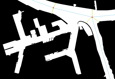
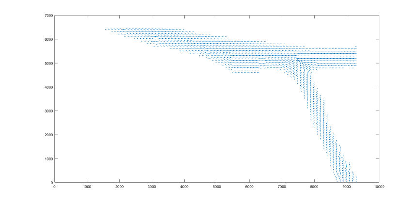
Another part of the script calculates the current in the Botlek area resulting from currents in the Oude Maas (Vertical river) & Nieuwe Maas (Horizontal river). The current is a very rough approximation for speed. It is based on a combination of laminar flow and self determined straight major flow lines which determine the angles. The angles are 'smoothed' to give a more realistic general flow pattern. This is done by taking into account the coordinates of calculation and its relative placement in relation to: | |||
- The major straight flow lines | |||
- The shore and its angle | |||
- Smooth lines ( in Map_calculation_lines.png: Blue lines / shore (and its angle) / Green lines ) | |||
The closer to the major flow-lines the more the speed equals 1m/s and the closer towards the shore the more the speed equals 0.36m/s. For the angles the overall angle of a coordinate is determined by how close the major flow-lines, smoothlines or shore is in relation to the coordinate. Where the closer it gets towards one of these the more its angle determines the overall angle of the coordinate. | |||
Each data point with water contains a current velocity value [m/s] and an angle value [Radial]. | |||
With angles being relative to unite circle orientation and the velocity being positive in the angle direction. The image on the right shows these currents in the river with the overall map on the left for comparison. | |||
[[File:Map_calculation_lines.png|500px]][[File:botlek_current.png|700px]] | |||
==== pH ==== | |||
The pH-values are also predefined, since the values differ per pixel. If those values would have to be calculated in the simulation, a lot of the total computation time would be used on this operation. To add some sort of randomness, three separate pH matrices are made, and for every time step one of these three matrices are chosen to be the pH present on the map. The values given to all the pixels are chosen by picking a value from a normal distribution, with a mean of 8.388 and a standard deviation of 0.004 [1]. The script to make those matrices could also be used for other pollution related that have to be measured in order to find a conclusion whether there's pollution or not. | |||
Source: [1] Gast, J.A.. REPRODUCIBILITY OF PH MEASUREMENTS IN SEAWATER. Department of Oceanography, Humboldt State College, Arcata, California. Retrieved from http://www.aslo.org/lo/toc/vol_11/issue_3/0417.pdf | |||
==== pH-contaminations ==== | |||
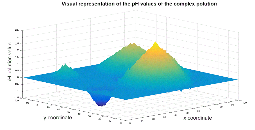
Creates an initial pollution and then creates a matrix containing this data which will then change over time depending on current and wind speed. This creates a pollution that has to increase or decrease the value of the overall pH-matrix. Swarm observation threshold for the final simulation should be 8.388 +/- 0.5. So values below 8.388-0.5 or above 8.388+0.5 are considered to be a pollution. | |||
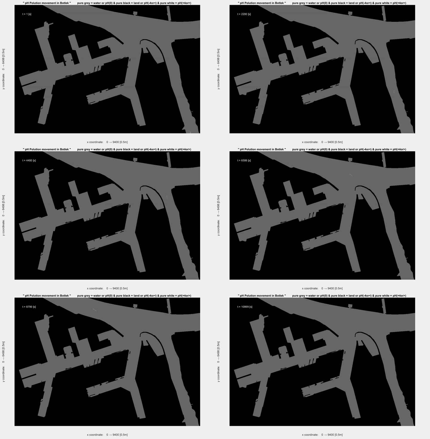
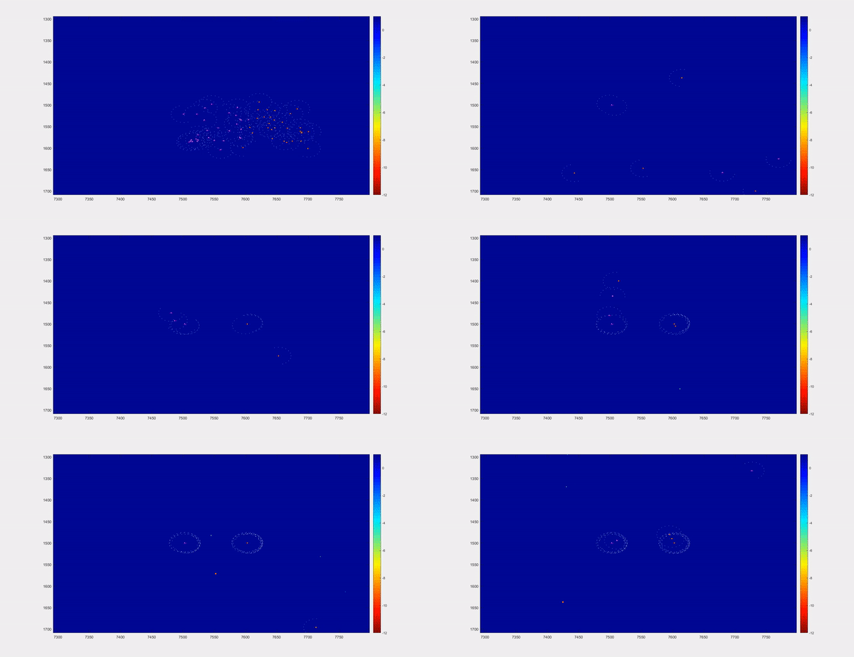
Here a pollution is visualized. On the left there is an image of how a pH pollution is defined in the simulation. On the right a video is placed where a contamination enters the system on the bottom right corner of the system and then moves through the river. | |||
[[File:pH-pollution.png|500px]][[File:PHPolution.gif|750px]] | |||
==== Day/Night cycle ==== | |||
The length of a day/night cycle differs per day of the year. Considering when this part of the script was made, 22 December[2], the shortest day of the year was chosen to model the cycle. Realistically, the curve which gives the light level varies per day. Since in the simulation one time step equals one second of simulation time, a day consists of 24*60*60 time steps, which is 86400 time steps. From 16:30 till 7:30, no light is present, and from 7:30 till 16:30, the function of the light follows half of a sine period, with a peak at 12:00 with an amplitude of 200Wm-2. | |||
Source: [2] Burgess, P. (2009, 29 september). VARIATION IN LIGHT INTENSITY AT DIFFERENT LATITUDES AND SEASONS, EFFECTS OF CLOUD COVER, AND THE AMOUNTS OF DIRECT AND DIFFUSED LIGHT. Retrieved from http://www.ccfg.org.uk/conferences/downloads/P_Burgess.pdf | |||
==== Wind ==== | |||
Wind direction is based on the probability of a certain wind direction on a given day, based on real life data[3]. A random value is generated every 10800 time steps (this value can be changed in the simulation), which when generated will determine the wind direction. A normal value with a mean of 10 and a standard deviation of 0.5 is chosen for the wind strength. | |||
Source: [3] https://www.windfinder.com/weatherforecast/rotterdam_airport | |||
==== Boats ==== | |||
Boats are implemented in the simulation in order to see the swarm's behaviour when encountering other traffic. There's only one size boat in the simulation, namely a container ship which has a length of 367m (734pixels) and a width of 50m (100pixels). This ship has two routes, in one route the boat will start in the port, in the southwest part of the map, and will go towards sea, which is at the northwest part of the map. In the other route, this route is reversed. The boats and its routes can be clearly seen in the simulation video. The swarm will have to avoid the boat, and not the other way around. Also, the swarm should be careful when the boat turns, since the boat is fairly long, the ends of the boat rotate fast. | |||
{| cellpadding="10" | |||
|-valign="top" | |||
|width="49%"| | |||
==== Driftwood ==== | |||
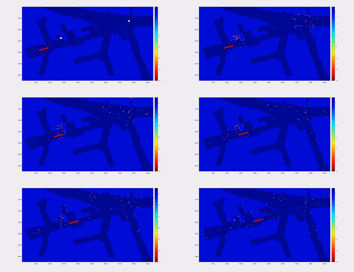
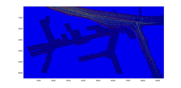
The driftwood part of the script is quite important for the simulation, considering the goal of the simulation is to remove those pieces of wood. There are 4 different sizes of driftwood in the simulation, namely (in pixels) 1x1, 2x1, 2x2 and 3x2. Every t, a random value gets generated, which decides whether one of those pieces will spawn if one were to spawn at all. The spawn rates of the driftwood can be changed easily, and do not have to be taken uniformly for the different sizes of driftwood. All of the pieces spawn in a random location where there is water, and when they do they receive an ID number. The ID numbers are separated for the different sizes of wood. The pieces get assigned an integer value, based on the size of the piece. This value is 4, 6, 8 and 10 for the sizes respectively. By subtracting these values from the map matrix, the swarm can read driftwood and also its size from the map. The movement of the driftwood per time step t is dependent on the current vector of the position of the piece, and also on the wind vector. In the figure, the traces of different pieces that spawned can be observed. | |||
|width="2%"| | |||
|width="49%| | |||
[[File:CurrentUSE.png]] | |||
|} | |||
=== Swarm === | |||
The swarm system implemented in our simulation is very useful for the fast exploration of different types of water surfaces, such as lakes and rivers in all sort of shapes and sizes. Depending on the size of the surface you wish to explore, you might want to increase the size of the swarm. It could also be desired to use multiple swarms, to explore the area in less time. For our simulation usually two swarms, consisting of 30 drones each, were used in different position of the Botlek part in the Rotterdam harbour. The purpose of our swarm, however, is not only to explore the area, but then to check if any pollution, in and on the water, is present. When the pollution is placed on top of the water, our drones will cooperate to remove these obstacles. | |||
Each swarm consists of 30 robots which all have one of three different types, the amount of each can be determined before running the simulation. Apart from different behaviour when near the shore, all robot types act the same. It is still very useful to have 3 different robot types, because it enables multiple forms of exploration and makes it easier for the swarm to adapt to different situations. | |||
Type 1: This robot type will follow the shore upon contact. This means that it follows a certain path while staying close to the shore, either on the left or the right side of the drone. Even when a corner comes, it will still follow this. This robot type is especially useful to implement in areas with complex geometrical structures, because it enables the robot to always escape these areas. It is also great for places where it is dangerous if anything is in the middle of the water, such as boat routes. | |||
Type 2: This robot type will act similar to type 1 at first and follow the shore, but whenever a turn appears, this type of robot will move straight ahead, this is really useful to have in your swarm when there are a lot of places where multiple rivers come together or there are a lot of small islands in the water, where type 1 would keep turning circles around. Similar to type 1 it is also great to implement in places where the middle is dangerous, however type 1 would stay safer. | |||
Type 3: When in contact with the shore, this type of drone will ‘bounce’ of the shore, with an angle equal to the angle it arrived. This type of drone is most likely to be implemented in large areas of water or wide rivers. | |||
Although each robot type has different qualities, it is advised to at least have a couple of each type in your swarm. | |||
{| cellpadding="10" | |||
|-valign="top" | |||
|width="49%"| | |||
There are two major ways the swarm communicates. The first communication happens during the exploration mode, where each robot makes sure it stays close enough to at least one other robot and at the same time keeps close enough to the center point of the swarm. Whenever it moves too far away, the robot will turn around to the center point of the swarm. | |||
The second form of communication happens whenever a drone finds an obstacle, the drone will then communicate to the other robots, whether it is able to move the object by itself or not. If it is not able too move the object by itself it will call the nearest available drone for help, this will continue until there are enough drones present to move the object. Then they will move the object to a hub, where the object will be removed from the water. | |||
In the video on the right a closeup is made of the swarm, here it can be seen how a drone calls for help if needed to remove a piece of driftwood from the system. This can also be found on youtube using the following link: https://www.youtube.com/watch?v=rq5HH48gL3Y | |||
|width="2%"| | |||
|width="49%| | |||
[[File:simulation_closeup.gif]] | |||
|} | |||
== Results == | |||
The generated data of 4 different simulations are analysed. These simulations are all done for the same amount of robots and the same ratio's in robot type. | |||
The simulations can be found in the zip file under 'results'. The most important result is when we compare the amount of wood that is in the maximum range of the swarm and how much of that wood is actually found by the robots. This percentage is dependent on where the robots are situated. When the robots are all situated in the Botlek, where only wind influences the wood, this percentage can be quite high. In the best case 60-80 percent is collected. The result is completely different when the robots are all situated in the main river where the water stream plays a large role. In this case we only got a percentage of 17-25 percent. | |||
Another important factor is the response time of the robots. This tells how fast the robots find the wood after it has spawned. We see the tendency that the robots in the Botlek initially have a higher response time than the robots in the main river. This can be explained by the fact that the wood flows towards the robots in the river. However there are some very high peaks in the double river position of the swarm. The robots are so busy with the salvaging with the huge amount of wood that it over reaches the swarm capacities. This could also explain the fact that much less wood in the river area is found that is in range of the robots. The robots are overworked in the main river. They get more wood to process than they can handle. | |||
The last value we have looked at is the waitingresponse time, which tells how much time is needed for the second or even third robot to arrive at the woodlocation. | |||
The waitingresponse time values for the 2x2 blocks are much lower then those for the 3x2 blocks. This can be explained by the fact that 2 robots are always close together but the third one doesn't have to be that close. Making the waitingresponse time for the 3x2 blocks much larger. The waitingresponse time in the river is generally larger than in the Botlek. This can be explained by the fact of the large amount of wood, when robots go out of the hub in the river they encounter wood much faster, this also results in more woodblocks where more robots are needed. This location is generally much closer to the hub than with the situation in the Botlek. The nearest robots are thus much faster at the required location. But this also means that less robots are available for searching again explaining the higher responsetimevalues and the lower percentage of the wood found that is in range. Because the most important task is helping other robots. | |||
In future research this could be changed by playing with parameters like the amount of robots and how they distribute tasks. Our simulation provides this basis and could be worked on in the future for more complex and multitask situations. | |||
= Week 1 = | = Week 1 = | ||
The goal of the first week was to decide on a subject for our project and what we were planning to do with this. This started on Monday with the first lecture, where we got more information about the course itself. After this we started brainstorming about different possible ideas to look into. A few examples of the things we looked at were space-exploration, robotic prosthetic and automating hazardous professions like firefighting. In the end we decided on swarm technology. We did still have to specify this so after the meeting we individually looked into some different applications of swarm technology. In the second meeting (17-11) we decided on a final subject: using swarm technology to observe the environment, focused on water like harbors and rivers. Here we want to test the quality of the water by looking at Chemicals, temperature, pH and metals. We decided on making a simulation of the system which can eventually be expanded. The next step was to figure out exactly what we need to make the simulation as realistic as possible, the USE-aspects and how we are going to approach the goal we set for ourselves. Our next meeting (19-11) was focused on combining the results we made throughout the week into a presentation that was to be given the following | The goal of the first week was to decide on a subject for our project and what we were planning to do with this. This started on Monday with the first lecture, where we got more information about the course itself. After this we started brainstorming about different possible ideas to look into. A few examples of the things we looked at were space-exploration, robotic prosthetic and automating hazardous professions like firefighting. In the end we decided on swarm technology. We did still have to specify this so after the meeting we individually looked into some different applications of swarm technology. In the second meeting (17-11) we decided on a final subject: using swarm technology to observe the environment, focused on water like harbors and rivers. Here we want to test the quality of the water by looking at Chemicals, temperature, pH and metals. We decided on making a simulation of the system which can eventually be expanded. The next step was to figure out exactly what we need to make the simulation as realistic as possible, the USE-aspects and how we are going to approach the goal we set for ourselves. Our next meeting (19-11) was focused on combining the results we made throughout the week into a presentation that was to be given the following Monday. | ||
[[File:Presentation_week1.pdf]] | [[File:Presentation_week1.pdf]] | ||
| Line 60: | Line 204: | ||
Orange = Stijn<br/> | Orange = Stijn<br/> | ||
Yellow = Ralf<br/> | Yellow = Ralf<br/> | ||
Blue = Stefan | Blue = Stefan<br/> | ||
Red = Koen & Zjeraar | Red = Koen & Zjeraar | ||
| Line 87: | Line 231: | ||
== Simulting the Environment == | == Simulting the Environment == | ||
=== Creation of | === Creation of 2D-space === | ||
In order to create a map for our simulation, we choose to render a map of the harbor into Matlab (we choose a piece of the harbor of Rotterdam called the Botlek). To do this a map of the harbor was taken and firstly edited a bit. The resolution was enhanced, smoothed out and colour-contrast was increased. Using a special script this was then translated into black-and-white picture of the map. This script gives all coordinates of water a value of 1 and the rest a value of 0. After this the resulting Matrix was doubled in size on both axis. | In order to create a map for our simulation, we choose to render a map of the harbor into Matlab (we choose a piece of the harbor of Rotterdam called the Botlek). To do this a map of the harbor was taken and firstly edited a bit. The resolution was enhanced, smoothed out and colour-contrast was increased. Using a special script this was then translated into black-and-white picture of the map. This script gives all coordinates of water a value of 1 and the rest a value of 0. After this the resulting Matrix was doubled in size on both axis. | ||
=== Space Data === | === Space Data === | ||
For the basic conditions of the environment, parameters are given to the matrix created in the | For the basic conditions of the environment, parameters are given to the matrix created in the 2D-space. | ||
| Line 105: | Line 250: | ||
Day/Night-cycle | Day/Night-cycle | ||
To simulate this, the black content matrix (used in the creation of the | To simulate this, the black content matrix (used in the creation of the 2D space) is multiplyied with an appropriate light intensity value, changing over time. This is saved as a new matrix. | ||
== Swarm system == | == Swarm system == | ||
| Line 186: | Line 331: | ||
Meanwhile in the simulation, a script was made to combine the different movements of the drones. This results in an algorithm for the swarm to form a path in the harbor of Rotterdam. | Meanwhile in the simulation, a script was made to combine the different movements of the drones. This results in an algorithm for the swarm to form a path in the harbor of Rotterdam. | ||
[[file: Notes_19-12.pdf]] | |||
As usual, the following link leads to our Dropbox files for this week. | |||
Week 6: [https://www.dropbox.com/sh/fpilrsrxd8flr6f/AACRx7m1v2zrtDKElbF_xKeKa?dl=0] | |||
{| cellpadding="10" | |||
|-valign="top" | |||
|width="49%" style="border:2px solid #2E9AFE;text-align: justify;background-color:white"| | |||
<h1 style="font-size:180%; border:none; margin:0; padding:0"> | |||
''Christmas break'' | |||
</h1><br/>During the christmas break work on the case and the simulation will continue, however due to other activities the progress we make might not be documented here on the wiki as well as previously. If this is missing at the end of the break, an update will be made to include the work done during the holidays. | |||
<br/> | |||
|} | |||
= Week 7 = | |||
Technically week 8, but we decided to not skip a week in our counting. | |||
Not a lot of work was done during the holidays, but were immediately picked up in the first week of the new year again. This included a visit to Rijkswaterstaat (RWS) in Echt near Sittard for more information and a lot of work on the simulation itself. | |||
== Rijkswaterstaat == | |||
On the 4th of January, Ralf, Zjeraar and Stijn had a meeting with people of the RWS on one of their patrol boats to ask some questions that could be useful for our design. Although hesitant at first, it turned out that the people of the RWS saw some really nice use for the system we are designing. Not only for what we already had in mind, but they also gave some examples of other way the system could be used. This gave a nice boost to the viability of our system since it turned out to be able to applied in a lot more situations on a lot more locations. Some of the examples they gave were for instance to not only use the drones to move driftwood, but also pieces of ice, or to help find missing persons in the water (which turned out to be needed quiet frequent). | |||
We had a number of questions we asked them to gain more insight into how the quality of the water is being controlled at the moment, how driftwood or other objects form a problem on the water and how this gets solved. It was also explained how the regulations work in regards to pollution of the water and how our system could help here. | |||
== Simulation == | |||
Meanwhile in the simulation work continued. The team responsible for simulating the environment added scripts to simulate driftwood in the water and how this moves through the system thanks to flow and wind. This was also done for pollutions, these can now be added to the system which then calculates and shows how these move and change in the rivers of our environment. At the moment this was done for pollutions altering the pH-value of the water but this can easily be copied to be applied to change the electro-conductivity or oxygen concentration of the water. | |||
The swarm team ran into some difficulty though, this is still behind schedule and although progress is being made, it is going slower than anticipated. At the moment scripts were made to have the swarm divide itself and prioritize certain tasks and the movements of the drones are finalized. One of the hurdles that were found was to have a drone that looking around for driftwood to determine the exact location of a piece of wood, instead of just acknowledging wood being in its vicinity. | |||
For more information about the progress of the project the notes of our last meeting and link to the dropbox folder for this week were added again. Please also note that on the top of the page there is also a link added to the folder of the simulation itself, this way the scripts which have more explanation about their progress can be seen for more clarity. | |||
[[file: Notes_08-01.pdf]] | |||
As usual, the following link leads to our Dropbox files for this week. | |||
Week 6: [https://www.dropbox.com/sh/xak8q32wcsupz8l/AACg5B4c1zzHOK68RJaBtgcYa?dl=0] | |||
= Week 8 = | |||
This is the final week to work on the simulation and this is what we focused heavily on. A lot of work still needed to be done to finish the script for the swarm. This then had to be combined with the script for the environment and the combination has to be run in order to get results. These results then had to be analysed and all of this had to be put together in order to present it on Monday the 16th. We had multiple meetings during the week to make sure everything was finished. Of these meetings only our meeting on Monday the 9th had notes made of them which are linked here. | |||
[[file: Notes_09-01.pdf]] | |||
Latest revision as of 12:24, 23 January 2017
| |||||||||||
|
You can click the following link for more background information on the course and the project. This link leads to the studyguide that was placed on oase. Final explanationHere will be a final explanation of all the different aspects of the project. Not only of the simulation but also of the contact with the projected users, the requirements and the choice for our system, These last two can be found in the files added here. The first of these is a full list of the requirements made for the system. The second is an explanation why swarm robotics is used for our problem instead of other options. Evaluation USE aspectIn the last couple of weeks our group encountered how much of an impact the user can have on the design of your technology. We started as a group wanting to do something big. Our common interest came down to a swarm technology, at first for exploring unknown places like Mars or the deep parts of the Ocean. But soon we came to the conclusion that we really need to have a good defined problem in order to go further with our swarm technology. We came up with the idea to monitor large bodies of water in industrialized areas on heavy pollution. We started to look and ask around. We contacted companies like Rijkswaterstaat, de Waterschappen the harbor police of Rotterdam and some others. At first glance these companies were interested but when asked what the real problems are they could not give a concrete answer. Until we made contact with a police officer from Rotterdam who would like to help us. He said that driftwood in the harbor of Rotterdam was a noticeable problem for his colleagues. It looked like we had found a real problem. But the question that arose was: how big is this problem. The police agent gave us a new contact to help us further. This was the Environmental police of Dordrecht. This police agent was very interested and gave us some deeper insight into harbor pollution. They have strict rules on water pollution which has improved the water quality greatly over the last 20 years. But for further insight he brought us in contact with another colleague. He told us that pollution was incidental and the same with driftwood. The problem of driftwood was in his eyes not a very big problem. But to get a real feeling of how pollution monitoring works he brought us in contact with someone from Rijkswaterstaat to make an appointment with 2 sailors who monitor the Maas river in Limburg. We had an interview with them which cleared a lot of things for us. The interview can be found in the pdf-file below. The interview gave us insight in what the problems really are, and this changed our goal for our swarm drastically. Instead of focusing on one particular problem like driftwood, we now focus on all different kind of objects in the water, from Big-Bags, plastics and wood to algae, and even (dead) bodies. This may not always form a dangerous problem for the big professional boats but does for the small recreational boats. This all has thought us that in order to come up with a good design constant interactions with the user is needed in order to prevent technocracy, which would lead eventually to a product that no one would use. SimulationAs explained before, the simulation is divided into two mayor parts: the environment and the swarm. This was done to independently focus on the proper working of the separate parts, which could then be combined to create a detailed whole. EnvironmentThe environment was again divided into sub-parts. These divisions were named the 3D-space (containing the map of the simulation), the source data (containing currents, pH-values, wind and day/night cycles) and finally the space-data containing driftwood, pollutions and other traffic. MapThe map on which the swarm operates, is a pre-made matrix in a script that reads an image, and based on the color of the image assigns a 1 or 0 per pixel. The image in the case of this project is an on top view of the Botlek harbour. This image was manually enlarged to ensure enough pixels would be present, since a scale can be assigned (real life distance per pixel) which should not be too small. With the chosen pixel size, namely 9400 width by 6498 height, a pixel is roughly 50 by 50 cm.
|
