Embedded Motion Control 2016 Group 2: Difference between revisions
| (154 intermediate revisions by 3 users not shown) | |||
| Line 13: | Line 13: | ||
|} | |} | ||
= ''' | = '''Introduction''' = | ||
The goal of the maze competition project is to create software that lets the pico robot solve a maze | The goal of the maze competition project is to create software that lets the pico robot solve a maze | ||
fully autonomous and as fast as possible. | |||
In this maze there will be certain obstacles | In this maze there will be certain obstacles | ||
that the robot has to overcome during the solving of the maze | that the robot has to overcome during the solving of the maze. Such obstacles are doors, open spaces, dead | ||
ends and loops. For more information on the maze challenge visit the | |||
ends and loops | [[Embedded Motion Control 2016| EMC 2016 Project Page ]]. | ||
= '''Group progress''' = | = '''Group progress''' = | ||
| Line 33: | Line 33: | ||
'''Week4''' | '''Week4''' | ||
:In this week a major shift occurred in our group. 2 group members left, and the code that we initially worked on was too complex. We decided to start from scratch, working on the basic software of the robot. Completing the corridor challenge was our main priority. We decided to use potential only in the x-direction to keep the robot positioned between the walls and avoid collisions. We didn't expect any problems in y-direction, so the speed in y-direction remained constant. A corridor detection was implemented based on the LRF data left and right from the robot. | :In this week a major shift occurred in our group. 2 group members left, and the code that we initially worked on was too complex and didnt work. We decided to start from scratch, working on the basic software of the robot. Completing the corridor challenge was our main priority. We decided to use potential only in the x-direction to keep the robot positioned between the walls and avoid collisions. We didn't expect any problems in y-direction, so the speed in y-direction remained constant. A corridor detection was implemented based on the LRF data left and right from the robot. | ||
'''Week5''' | '''Week5''' | ||
:In this week we combined the potential field, that was used to avoid collisions and keep the robot between the corridor walls, with corridor detection to obtain 3 states for the robot. One where a corridor is recognized on the left side with translational motion set to zero and where it keeps rotating until it faces the direction of the detected corridor. The second state is almost exactly the same as the previous one, it differs as the recognized corridor is on the right side of the robot. The third state is where it moves through the corridor with a constant speed in the y-direction, an alternating speed in the x-direction based on the potential field | :In this week we combined the potential field, that was used to avoid collisions and keep the robot between the corridor walls, with corridor detection to obtain 3 states for the robot. One where a corridor is recognized on the left side with translational motion set to zero and where it keeps rotating until it faces the direction of the detected corridor. The second state is almost exactly the same as the previous one, it differs as the recognized corridor is on the right side of the robot. The third state is where it moves through the corridor with a constant speed in the y-direction, an alternating speed in the x-direction based on the potential field. This was also the week of the corridor challenge, which we succeeded on the first try. The only point was that it moved to slow in the y-direction which is due to the unchanged parameter for the speed "Vy" we used during the tests. On the same day we had our intermediate presentation. Link to the presentation can be found at the bottom of this page under Files. | ||
'''Week 6''' | '''Week 6''' | ||
| Line 42: | Line 42: | ||
'''Week 7''' | '''Week 7''' | ||
:The implementation of potential field together with object detection and planning caused problems. When turning, object detection returned unreliable objects. Since object detection was required for the placement of the reference point, we could not disable object detection during turning. Therefore a new way of placing the reference point was developed. In more detail this is discussed in ' | :The implementation of potential field together with object detection and planning caused problems. When turning, object detection returned unreliable objects. Since object detection was required for the placement of the reference point, we could not disable object detection during turning. Therefore a new way of placing the reference point was developed. In more detail this is discussed in 'Limited range open-space detection' below. The new reference placement, together with the potential field, was tested and worked satisfactory on the real robot. Furthermore the final presentation was given, the PDF can be found under Files. The second part of the week the focus was on mapping. Planning could then use mapping to decide where to place the reference point based on the Tremaux's solving algorithm. | ||
'''Week 8''' | '''Week 8''' | ||
:Week eight was the week of the maze challenge. Mapping the maze was to complicated for us at this stage, therefore an alternative maze solving strategy was developed. For more detail see section ' | :Week eight was the week of the maze challenge. Mapping the maze was to complicated for us at this stage, therefore an alternative maze solving strategy was developed. For more detail see section 'Final planning'. Moreover, dead-end detection was added. At the beginning of the week the software was tested. Results were positive except for side-door detection. Minor changes to the code were made before the actual maze challenge. The robot did not complete the maze and bumped into a wall during both trials. For a more detailed report on the maze challenge go to the section 'The maze challenge'. | ||
= '''Initial design''' = | = '''Initial design''' = | ||
The PDF of the initial design can be found in the section | The PDF of the initial design can be found in the section Files. | ||
=== '''Requirements''' === | === '''Requirements''' === | ||
| Line 107: | Line 107: | ||
=== '''Interfaces''' === | === '''Interfaces''' === | ||
The software can be divided in 5 contexts: | The software can be divided in 5 contexts: | ||
| Line 128: | Line 122: | ||
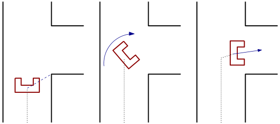
= '''The corridor challenge''' = | = '''The corridor challenge''' = | ||
The strategy to complete the corridor challenge was straightforward. Drive straight whilst staying in the centre of the corridor and take the first exit. | The strategy to complete the corridor challenge was straightforward. Drive straight whilst staying in the centre of the corridor and take the first exit. For more information on the corridor challenge visit the [[Embedded Motion Control 2016| EMC 2016 Project Page ]]. | ||
[[File:Corrchallengev2.png|right|frame|Left: Pico drives through the corridor until it detects an edge, in this case a right edge. Pico is given a state that he has to start turning after driving a certain distance.<br\> | |||
Middle: After driving a certain distance, Pico stops and starts turning 90 degrees clockwise.<br\> | |||
Right: Pico starts to drive again, while the potential field aligns the robot between the two walls again.]] | |||
=== '''Components''' === | === '''Components''' === | ||
The following components were used to complete the corridor challenge: <br\> | |||
* Potential field: | * Potential field: | ||
:A simple but robust sideways potential field that keeps the robot in the center of the corridor. | :A simple but robust sideways potential field that keeps the robot in the center of the corridor. | ||
* Corridor recognition: | * Corridor recognition: | ||
:Corridor recognition based on jumps in laser range data | :Corridor recognition based on jumps in laser range data. | ||
* A state switch | * A state switch: | ||
:After recognizing the corridor and being within a certain range, a new state is activated. In this state the robot drives to the middle of the corridor. Then the robot turns and aligns itself as good as possible with the corridor based on | :After recognizing the corridor and being within a certain range, a new state is activated. | ||
:In this state the robot drives to the middle of the corridor. Then the robot turns and aligns itself as good as possible with the corridor based on odometry data. | |||
=== '''The result''' === | === '''The result''' === | ||
Pico successfully completed the corridor challenge using the strategy described above.<br\> | Pico successfully completed the corridor challenge using the strategy described above.<br\> | ||
A note worth mentioning was that the default velocity was low. This was a safety decision made by the group since this was also the speed used for testing. Theoretically the default speed should not have influenced the robustness of Pico. Moreover, during the challenge, | A note worth mentioning was that the default velocity was low. This was a safety decision made by the group since this was also the speed used for testing. <br\> | ||
Theoretically the default speed should not have influenced the robustness of Pico. Moreover, during the challenge, it became clear that velocity could have been significant higher velocity. | |||
= '''Final implementation''' = | = '''Final implementation''' = | ||
In this section the final software is presented. However, also previous ideas and implementations are discussed to show the design choices made in the process. | |||
== '''Software architecture''' == | |||
[[File:software_arch.png|upright=2.25|right|thumb|Software architecture]] | |||
The maze solving problem is being tackled with six functions that are shown in the blocks in the diagram to the right. | |||
* The data from the laser range finder and the odometry are collected. | |||
* Based on the odometry data and a prediction, the global position of the robot can be estimated. | |||
* With help of the data collected from laser range finder corners and various types of conjunctions can be detected. | |||
* Certain points in the maze are derived from the localization are registered, these registered points form a map of the maze. | |||
* Combining the results from the mapping and object detection, decisions are made on where to set the reference point based on the type of conjunction and whether a location has already been visited. | |||
* The potential field creates virtual forces to attract the robot to a reference point while avoiding collisions with walls by means of repulsive forces. From these forces velocities are calculated which are send to the robot. | |||
* The drive function decides whether to collaborate with these speeds calculated from the potential field based on type of conjunction and corridor. | |||
<br /> | |||
<br /> | |||
<br /> | |||
<br /> | |||
<br /> | |||
== '''Potential field''' == | |||
To prevent the robot from colliding with the wall, a potential field was used. The potential field consists of an attractive field and an repulsive field, | |||
which when the two fields are combined, results in an evasive motion of obstacles. | |||
===Repulsive field=== | |||
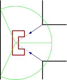
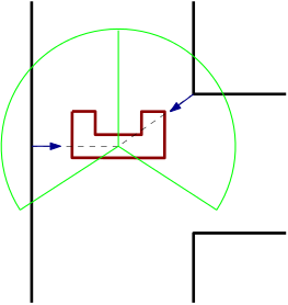
We made a choice to split our potential field in a left and right field and only use two vectors for a potential field as can be seen in the figure below. | |||
In each field the vector was determined by checking the minimum range. This leads to a minimum range vector for the left side and a minimum range vector for the right side. | |||
Adding these vectors to each other leads to a repulsive force in the x direction and the y direction relative to the robot. | |||
Scaling these forces gives us velocity Vxr in the x direction and a Vyr in the y direction | |||
===Attractive field=== | |||
The attractive force is determined with the reference point given by the planning block, which is considered as a vector. | |||
With this vector the angle difference between reference vector and the front of the robot is calculated. This difference is scaled and used to give the robot a rotation velocity named ome. | |||
The robot itself is given a constant initial velocity Vyi in the y direction to drive. | |||
===Combined field=== | |||
The final velocities Vx, Vy and Ome are calculated by adding the repulsive field to the attractive field. | |||
When the robot is driving straight to a wall, the repulsive velocity Vyr negates the initial velocity Vyi to nearly zero. | |||
When the robot slowly drives to the wall and gets close, the safety feature kicks in and rotates the robot 45 degrees. | |||
{|200px|style:"margin: 0 auto;" | |||
|[[File:potfield.png|frame|right|Repulsive field in front of a corridor with 3 options]] | |||
|[[File:potfield2.png|frame|right|Repulsive field in front of a corridor with 2 options]] | |||
|} | |||
== '''Detection''' == | == '''Detection''' == | ||
In this section the detection of several objects is discussed. In landmark detection objects such as junctions, t-crossing, corners and corridors are detected. Two special objects, the dead end and the side door, are specifically addressed since they differ from the other landmarks. Furthermore, a second method to detect possible corridors is presented in Limited range open-space detection. | |||
=== Landmark detection === | === Landmark detection === | ||
Landmark detection is used to detect the object and type of object ahead of the robot.These objects are then passed to planning, which decides where to place the reference point.<br /> | |||
<br /> | |||
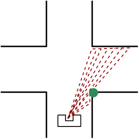
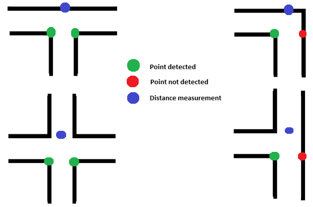
Object detection is based on three points. A point is detected by looking at jumps in laser range data as shown in the left figure below. This way the robot tries to detect the bottom right and bottom left point of an object. Furthermore the robot scans for the point straight ahead. Depending on what points are actually detected, the algorithm determines the kind of object. For example, the top left situation depicted in the right figure below. Both bottom left and right point are detected by a jump in laser range data. When scanning straight ahead, a wall is found. This means that the only possible object is a t-crossing. | |||
{|style:"margin: 0 auto;" | |||
|[[File:Point_Detection3.png|upright=2.25|thumb|right|Point detection used for object detection]] | |||
|[[File:Objects_Group2.png|upright=2.25|thumb|right|Three point object detection method]] | |||
|} | |||
=== Dead end detection === | |||
When at least 95% of all LRF points is smaller than a predefined range, detection | When at least 95% of all LRF points is smaller than a predefined range, detection passes the variable object the number that corresponds with a dead end. | ||
This results in the dead end protocol | This results in the activation of the dead end protocol. In this protocol Pico stops 0.4m in front of the dead end wall, beeps, and waits 5 seconds. After these 5 seconds, it looks if a door is opened or if it still is a dead end. | ||
If object number still shows dead end, Pico turns 180 degrees and continues to drive. If a door was opened, Pico will continue the new path.<br /> | If object number still shows dead end, Pico turns 180 degrees and continues to drive. If a door was opened, Pico will continue the new path.<br /> | ||
<br /> | <br /> | ||
| Line 171: | Line 217: | ||
|} | |} | ||
=== Side door detection === | |||
[[File:sidedoordet.png|frame|The global position of the robot within a certain reference frame|right]] | |||
Because we use the limited LRF to place our reference points in open spaces, a side door is harder to detect. For these side doors a protocol was written to still detect these doors.<br\> | Because we use the limited LRF to place our reference points in open spaces, a side door is harder to detect. For these side doors a protocol was written to still detect these doors.<br\> | ||
<br\> | |||
When the robot drive through a corridor it keeps scanning a small set of points left and right for a sudden change in LRF range. When it detects a sudden change, the algorithm will check if the x values with reference to the robot lie within a certain tolerance. This was done respectively for the points after the sudden change and for the points before. This was done to make it more robust to ,for example, small gaps in a wall. | When the robot drive through a corridor it keeps scanning a small set of points left and right for a sudden change in LRF range. When it detects a sudden change, the algorithm will check if the x values with reference to the robot lie within a certain tolerance. This was done respectively for the points after the sudden change and for the points before. This was done to make it more robust to ,for example, small gaps in a wall. | ||
<br /> | |||
{|style:"margin: 0 auto;" | {|style:"margin: 0 auto;" | ||
|[[File:Rightdoor.gif|frame|Right door detection]] | |[[File:Rightdoor.gif|frame|Right door detection]] | ||
|[[File:Leftdoor.gif|frame|Left door detection]] | |[[File:Leftdoor.gif|frame|Left door detection]] | ||
|} | |} | ||
=== | === Limited range open-space detection === | ||
To | To detect possible corridors more robustly, a variable limited LRF range was used. By limiting the LRF range, possible open spaces which can indicate corridors can be detected, these can be seen in the figure below. | ||
<br /> | <br /> | ||
{|style:"margin: 0 auto;" | {|style:"margin: 0 auto;" | ||
|[[File: | |[[File:Limrangeleftstr.png|upright=2|thumb|Reference point placement with 3 potential corridors]] | ||
|[[File: | |[[File:Limrangev5.png|upright=2|thumb|Reference point placement with 2 potential corridors]] | ||
|} | |} | ||
<br /> | <br /> | ||
The | The pictures show the limited LRF range of Pico before a crossing. The grey area is where all the limited LRF points are equal to the set maximum range. The orange area is where the LRF data detects a point within the limited-LRF data. | ||
The open space detection looks at all the limited range data in a loop from right to left anti-clockwise and determines when a high number of consecutive points are equal to the limited range | The open space detection looks at all the limited range data in a loop from right to left anti-clockwise and determines when a high number of consecutive points are equal to the limited range.<br\> This area is an open space, thus a potential corridor. In the figure above this can be seen as the gray area. To prevent any small gaps to be detected, a minimum amount of conclusive points have to be detected in order to label it a potential corridor. <br /> | ||
<br /> | |||
Each time a potential corridor is detected, an x and y reference in the middle of the potential corridor at maximum range is stored. The first one detected is always saved as the first reference, the second one detected as the second reference etc, moving from right to left.<br\> This is also indicated with the numbers in the open-spaces in the figure above. | |||
When driving in an actual open-space, the maximum range of the LRF data is increased such that it can again detect potential corridors further away. The most right open-space is always the first reference, one open-space to the left the second etc. This can be seen in the figures above. | |||
<br /> | |||
<br /> | <br /> | ||
The source code can be found below in the section Code. | |||
== '''Localization''' == | == '''Localization''' == | ||
[[File:global.png| 50px|right|alt=A|frame| The global position of the robot within a certain reference frame.]] <br /> | |||
Being aware of the global position of the robot is critical for mapping and also useful for the motion of the robot. The global position of the robot is formulated as, <math>\begin{bmatrix} | Being aware of the global position of the robot is critical for mapping and also useful for the motion of the robot. The global position of the robot is formulated as, <math>\begin{bmatrix} | ||
x\\ | x\\ | ||
| Line 204: | Line 259: | ||
\theta | \theta | ||
\end{bmatrix}</math>. The figure below shows a graphical representation of the global position. <br /> | \end{bmatrix}</math>. The figure below shows a graphical representation of the global position. <br /> | ||
<br /> <br /> <br /> <br /> | |||
=== Discrete time model === | === Discrete time model === | ||
| Line 222: | Line 277: | ||
Where <math>V_x</math> is the sideward velocity, <math>V_y</math> the forward velocity, <math>\omega</math> the rotational speed and <math>\Delta{t}</math> the duration of each time step in the discrete model. | Where <math>V_x</math> is the sideward velocity, <math>V_y</math> the forward velocity, <math>\omega</math> the rotational speed and <math>\Delta{t}</math> the duration of each time step in the discrete model. | ||
<br /> | |||
<br /> | |||
=== '''Extended Kalman filter''' === | === '''Extended Kalman filter''' === | ||
| Line 231: | Line 288: | ||
The discrete time model of the global position that was mentioned before is being used as the prediction model for the global position. The input data are the forward speed, sideward speed and rotational speed calculated by the code and giving to ''io.sendBaseReference()''. Combining the prediction model and the input data will give an estimation of the global position of the robot. To get a proper estimation of the global position, the measurement noise and the process noise need to be modelled correctly. The measurement noise can be based on sampling experimental data and deriving the statical properties. The covariance matrix <math>R</math> of the measurement noise can be calculated by, | The discrete time model of the global position that was mentioned before is being used as the prediction model for the global position. The input data are the forward speed, sideward speed and rotational speed calculated by the code and giving to ''io.sendBaseReference()''. Combining the prediction model and the input data will give an estimation of the global position of the robot. To get a proper estimation of the global position, the measurement noise and the process noise need to be modelled correctly. The measurement noise can be based on sampling experimental data and deriving the statical properties. The covariance matrix <math>R</math> of the measurement noise can be calculated by, | ||
<math>R_{ij} = \frac{1}{N-1}\sum_{k=1}^{N}(x_i-\bar{x}_i)(x_j-\bar{x}_j).</math>.<br/> | |||
The covariance matrix <math>Q</math> which represents the process noise is not as straightforward as the covariance matrix for the measurement noise. It is being used to filter the errors in system model. Therefore the covariance matrix <math>Q</math> is being treated as a tuning parameter. | The covariance matrix <math>Q</math> which represents the process noise is not as straightforward as the covariance matrix for the measurement noise. It is being used to filter the errors in the system model. Therefore the covariance matrix <math>Q</math> is being treated as a tuning parameter. A piece of the code that is used for the extended kalman filtering is shown below. | ||
[[File:Kalman.png]] | //=====================Prediction========================= | ||
// State estimation | |||
x[2] = x_[2] + omega/freq; | |||
x[0] = x_[0] + Vx/freq*cos(x[2]) - Vy/freq*sin(x[2]); | |||
x[1] = x_[1] + Vx/freq*sin(x[2]) + Vy/freq*cos(x[2]); | |||
x_[0] = x[0]; | |||
x_[1] = x[1]; | |||
x_[2] = x[2]; | |||
// Covariance estimation | |||
P = J*P*transJ+Q; | |||
//===================Updating============================= | |||
// Measurement residual | |||
y[0] = deltaodomx-Vx/freq; | |||
y[1] = deltaodomy-Vy/freq; | |||
y[3] = deltaodoma-theta/freq; | |||
// Innovation residual | |||
Mat S = H*P*transH+R; | |||
// Kalman gain | |||
Mat K = P*transH*S.inv(); | |||
// Updated state estimation | |||
Mat xest = x+K*y; | |||
// Updated covariance estimation | |||
P = (Mat::eye(3,3,CV_64F)-K*H)*P; | |||
The extended Kalman filter follows the following scheme to estimate the global position of the robot. <br/> | |||
[[File:Kalman.png|frame|center|Extended Kalman scheme]] | |||
Unfortunately, the data collected from the experiments did not seem trustworthy, and there were no more opportunities to test these results. From there on a decision was made not to use the estimations calculated from the Kalman filter. | |||
== '''Mapping''' == | == '''Mapping''' == | ||
[[File:mapping3.png| | [[File:mapping3.png|thumb|upright=3|right|alt=A | Mapping the maze using previous positions]] | ||
The idea of mapping is to memorize certain points in the maze. This would be used to solve the maze, as the code would tell whether the robot had already visited certain locations in the maze. The initial idea was to save the positions of landmarks of maze, in this case corners of the corridors and points that are used to recognize conjunctions. This has proven to have some difficulties. This is why a decision has been made to map the maze with another method. This method is pretty straightforward. Every two seconds during the maze solving it registers the current position of the robot, see the left picture for a graphical representation where the red dots represent the registered positions. These positions are saved in a list which are used in the maze solving algorithm. | |||
In order to solve the maze, the locations the robots already visited need to be recognized. The recognition of visited locations is made possible by creating a virtual rectangular box between a saved position and its preceding saved position while it is being aligned with the corresponding corridor. The right figure above shows a graphical representation where virtual rectangular boxes are created between saved positions. So when a reference point is set in an area created by these boxes the code can recognize whether the location of the reference point had already been visited, this can contribute to the maze solving. | In order to solve the maze, the locations the robots already visited need to be recognized. The recognition of visited locations is made possible by creating a virtual rectangular box between a saved position and its preceding saved position while it is being aligned with the corresponding corridor. The right figure above shows a graphical representation where virtual rectangular boxes are created between saved positions. So when a reference point is set in an area created by these boxes the code can recognize whether the location of the reference point had already been visited, this can contribute to the maze solving. | ||
<br /> | |||
<br /> | |||
<br /> | |||
<br /> | |||
== '''Planning''' == | == '''Planning''' == | ||
Here the planning is addressed. The 'planned' planning is the planning such as it was initially designed for implementation. Due to difficulties however, this planning was replaced by the 'final' planning. | |||
=== '''The planned planning''' === | === '''The planned planning''' === | ||
The initial idea was the following. Detection gave the object ahead to planning. Planning had information about this object and previous object from mapping. Using this information, and the Tremaux's algorithm, planning placed a reference at a specific point. This system should have been able to solve the maze. However, difficulties in the implementation of mapping and object detection forced the group to develop an other strategy. | |||
=== '''The final planning''' === | === '''The final planning''' === | ||
The final decision making algorithm makes use of the limited range open-space detection. It creates a reference point at one of the open spaces. Initially, the preference is given to the right most open space. Following the right wall always ensures solving the maze, unless the robot starts in a loop. Therefore, another algorithm was developed that prevents the robot from staying in a loop. This algorithm is elaborated below.''' | |||
When Pico continues to turn to the right, planning will always pick the last reference point. | |||
'''Loop prevention'''<br\> | |||
The algorithm is based on the odometry data. An adjustment to the odometry data was made to make the data continuous, so without jumps. The planning block will have at most three potential reference points to chose from, right, middle or left. Initially Pico will always pick the first reference point, which will be the most right option. When Pico has turned a few times to the right, the planning block picks the second reference point when available. When Pico continues to turn to the right, planning will always pick the last reference point.<br\> | |||
So when the robot is in a loop by driving in a clockwise rotation, he will search eventually look voor a left corridor and pick this reference. <br\> | |||
If he keeps driving in an anti-clockwise rotation, he will look for an exit at the right after a few turns. | |||
Below is a video of the robot using this algorithm to get out of of a loop. | |||
{| | {| | ||
|[[File:loopsolve.png| | |[[File:loopsolve.png|right|300px|link=https://www.youtube.com/watch?v=EsTg2XHhD-M]] | ||
|} | |} | ||
= '''The maze challenge''' = | = '''The maze challenge''' = | ||
The maze | [[File:maze_design_final_challengeV2.png|right|frame|The final maze]] | ||
The maze from our maze challenge can be seen in the figure to the right. | |||
<br> | <br> | ||
=== '''The result''' === | === '''The result''' === | ||
Unfortunately we didn’t pass the Maze challenge itself. | |||
During the first attempt the robot recognized doors everywhere and the robot eventually collided sideways in a wall. | During the first attempt the robot recognized doors everywhere and the robot eventually collided sideways in a wall. | ||
During the second attempt the robot turned right, took another right and then continued the corridor | During the second attempt the robot turned right, took another right and then continued the corridor until it passed the door on the left and turned right again. Then Pico drove close to a wall, stopped and then bumped into it again. | ||
<br> | |||
<br> | |||
=== '''Evaluation''' === | === '''Evaluation''' === | ||
During both attempts, the planning block interfered with the driving. The planning block chooses a reference point out of all possible choices based on how many rotations the robot has made. | During both attempts, the planning block interfered with the driving. The planning block chooses a reference point out of all possible choices based on how many rotations the robot has made. To estimate the number of rotations Pico has made, the odometry data was used. When Pico made more than around 1.5 rotation to the right (540 degrees in comparison to the start condition), the reference point switched from first reference point to second. Unfortunately the switching criterion between picking the first or second reference was determined mid-cornering due to the odometry data already having an initial state at the start. This caused the Robot to simultaneously switch between picking the first and second reference, which lead to the robot driving to the wall between the reference points. | ||
To estimate the number of rotations Pico has made, the odometry data was used. When Pico made more than 1.5 rotation to the right. | On top of that, the potential field wasn’t scaled aggressively enough to prevent a side ways collision. <br/> | ||
This caused the Robot to | |||
On top of that, the potential field | |||
<br/> | <br/> | ||
=== '''Fixing the problem''' === | === '''Fixing the problem''' === | ||
To fix the problem described above, the potential field was scaled a bit more agressively. Furthermore, reference choice was made more robust by introducing a state. <br\> | To fix the problem described above, the potential field was scaled a bit more agressively. Furthermore, reference choice was made more robust by introducing a state. <br\> | ||
If Pico made more than 1.5 rotations to the right, a state was introduced that keeps picking the second reference point until the | If Pico made more than around 1.5 rotations to the right, a state was introduced that keeps picking the second reference point until the cumulative rotations of pico is zero again. <br\> | ||
When Pico makes more than 2.5 rotation to the right, another state was introduced to keep picking the last reference point until the | When Pico makes more than around 2.5 rotation to the right, another state was introduced to keep picking the last reference point until the rotation decrease to 1.5. After falling below around 1.5 rotations, the second reference point is picked again.<br\> | ||
Below is a video where Pico passes the Maze Challenge in the simulation. | This is shown in the code below.<br\> | ||
int corner=0; | |||
float oneandhalfrot=-9; // This is in radians and is a bit less than 1.5 rotations. | |||
float twoandhalfrot=-16; // This is in radians and is a bit more than 2.5 rotations. | |||
float resetrot1=-1; // This is a bit less than the starting condition. | |||
float resetrot2=-10; | |||
//Solving stategy for the maze. At first the robot will always take the most right reference point, | |||
//however, when a certain amount of clockwise rotation is passed, it will take the second reference point, if available. After even | |||
//more clockwise rotation the robot will take the last reference point available. | |||
//below is the code to determine which reference point to pick at the next crossing. | |||
if(odoma>0) | |||
{ | |||
cstate=0; //state for which the most right reference point is preferred. | |||
} //This is our choice making state. | |||
if(odoma<oneandhalfrot && odoma>twoandhalfrot &&cstate==0) //When this argument is satisfied the choice making state changes | |||
{ | |||
cstate=1; //state for which the second reference point is preferred | |||
} | |||
if (odoma<twoandhalfrot&&cstate==1) //When this argument is satisfied the choice making state changes again. | |||
{ | |||
cstate=2; //state for which the last reference point is preferred | |||
} | |||
if (cstate==1&& odoma>resetrot1) //When this argument is satisfied the choice making state resets to | |||
{ //the most right reference point again. | |||
cstate=0; | |||
} | |||
if (cstate==2&& odoma>resetrot2) //This argument resets the ref point preference from the last ref point to second. | |||
{ | |||
cstate=1; | |||
} | |||
//below is the code that couples the preferred reference point to the options that are available. | |||
//A corner state of 0 means that the most right option is preferred, which is always available. This is | |||
// each loop the inital state of corner. if the corner state is 1, it will directly pick the second reference point, | |||
//and when it is 2 it will directly pick the third reference point. | |||
//The difference between the choice making state and the corner state is that the choice state gives a preference, while | |||
//the corner state is based onthe combination of the available options and the preferred state. | |||
if (cstate==1) //When the choice state state is 1, this argument check wether there are more than | |||
{ //one options available. If this is the case, it will pick the second ref point. | |||
if(data2.nrop>1) //This state gives the actual number of options available. | |||
{ | |||
corner=1; | |||
} | |||
} | |||
if (cstate==2) // When the choice state is 2, this argument check wether there are more than | |||
{ //one options available. If there are two options, it will pick the second ref point, | |||
if(data2.nrop==2) //and when there are 3 options, it will pick the third reference ref point. | |||
{ | |||
corner=1; | |||
} | |||
else if(data2.nrop>2) | |||
{ | |||
corner=2; | |||
} | |||
} | |||
<br\> | |||
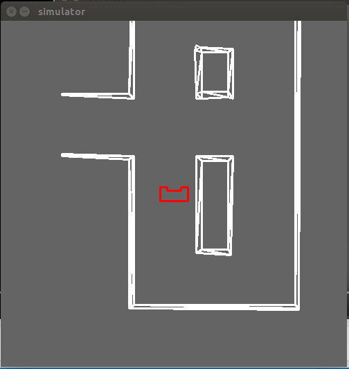
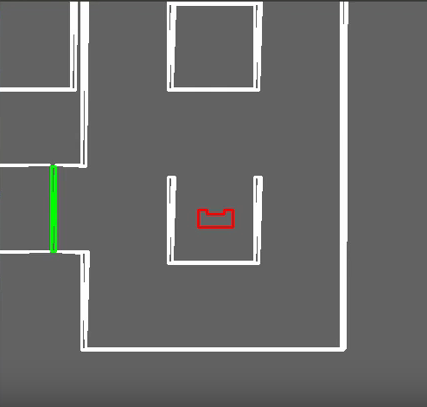
Below is a video where Pico passes the Maze Challenge in the simulation. In this simulation Pico first turns right every corner, until it drives into his starting position again. Pico has rotated 1.5 times, so now it follows the second reference point until it rotates back until his starting orientation is reached. Now Pico starts picking the first reference point again.<br\> He then drives into a dead end to check for a door, turns around and pick the right corner again. After a while he detect the door on his right, turns into the the corridor, turns right again. After reaching the open space he adjusts his maximum range to still see the walls and drives to the end. | |||
{| | {| | ||
| Line 288: | Line 454: | ||
|} | |} | ||
= '''Conclusion''' = | |||
Robustness is the key in unpredictable situations. Even though the robot successfully completed several test, during the maze challenge it bumped into a wall. Furthermore, thinking about the integration of individual pieces of code into the main software is critical for efficient programming. Design architecture and overall communication should be worked out before beginning the actual programming. Here are some more conclusions and experiences gathered: | |||
<br/> | |||
* Overall C++ programming | |||
* Working with GIT | |||
* Avoid magic numbers for scalability of the code | |||
* Simulations differ from the reality, therefore again robustness is required | |||
* First create a solid basic to work from, then expand | |||
* Clear and frequent communication between team members is critical for the progress of the group | |||
= ''' | = '''Recommendations''' = | ||
Due to a restart of the project and the limited manpower, there are certain elements we could not spend (enough) time on. The following would have been implemented or considered if there was time to improve the quality of the solution to the maze solving problem. | |||
* As mentioned before, the extended Kalman filter lacks a proper covariance matrix for the measurement noise due to dubious measurement data which could not be tested. A proper testing plan should have been created and the results from the testing should be evaluated by other tests. This would result in an extended Kalman filter of a higher quality. | |||
* There were problems with mapping where it did not tell if the location was already visited when it should. Visualisation of the mapping should be implemented. This could be a great asset in terms of debugging. | |||
* Making side door detection more robust. Sometimes the robot didn't recognize doors because our requirements were too strict. | |||
= '''Code''' = | |||
* Planning [https://gist.github.com/anonymous/0065b9c795db20c850c952b0aadd0c67 code] | |||
* Limited range detection [https://gist.github.com/anonymous/752dfdc9963354733cb566cc9a0753fa code] | |||
= '''Files''' = | = '''Files''' = | ||
* Initial design: [[Media:Initial idea group2.pdf|Initial | * Initial design: [[Media:Initial idea group2.pdf|Initial idea report]] | ||
* Intermediate presentation: [[Media:initialpresentation_emc.pdf| | * Intermediate presentation: [[Media:initialpresentation_emc.pdf|Intermediate presentation]] | ||
* Final presentation: [[Media:Final_Presentation_Group2.pdf|Final presentation]] | |||
Latest revision as of 23:35, 17 June 2016
Group Members
| 0779760 | Ilias Aouaj |
| 0818316 | Florian Bastiaens |
| 0755206 | Yannick Knops |
Introduction
The goal of the maze competition project is to create software that lets the pico robot solve a maze fully autonomous and as fast as possible. In this maze there will be certain obstacles that the robot has to overcome during the solving of the maze. Such obstacles are doors, open spaces, dead ends and loops. For more information on the maze challenge visit the EMC 2016 Project Page .
Group progress
Week 1
- During the first week all group members installed the required software. Furthermore a start was made with the tutorials.
Week 2
- The start of week two was all about the design plan. Discussed were the requirements, what functions to use, the specifications and the components. A quick overview of the initial design can be found at the bottom of this page. Moreover in week two the tutorials were finished.
Week 3
- Week three the actual coding started. Tasks were divided and a start was made on several aspects of the code.
Week4
- In this week a major shift occurred in our group. 2 group members left, and the code that we initially worked on was too complex and didnt work. We decided to start from scratch, working on the basic software of the robot. Completing the corridor challenge was our main priority. We decided to use potential only in the x-direction to keep the robot positioned between the walls and avoid collisions. We didn't expect any problems in y-direction, so the speed in y-direction remained constant. A corridor detection was implemented based on the LRF data left and right from the robot.
Week5
- In this week we combined the potential field, that was used to avoid collisions and keep the robot between the corridor walls, with corridor detection to obtain 3 states for the robot. One where a corridor is recognized on the left side with translational motion set to zero and where it keeps rotating until it faces the direction of the detected corridor. The second state is almost exactly the same as the previous one, it differs as the recognized corridor is on the right side of the robot. The third state is where it moves through the corridor with a constant speed in the y-direction, an alternating speed in the x-direction based on the potential field. This was also the week of the corridor challenge, which we succeeded on the first try. The only point was that it moved to slow in the y-direction which is due to the unchanged parameter for the speed "Vy" we used during the tests. On the same day we had our intermediate presentation. Link to the presentation can be found at the bottom of this page under Files.
Week 6
- Week six the main focus was on potential field and wall detection. The potential field used in the corridor challenge was too simplistic to provide robust collision prevention during the maze challenge. Repulsive forces in the y direction were added and scaling was improved. Furthermore object detection was implemented. Using object detection a reference point was placed by the function 'planning'.
Week 7
- The implementation of potential field together with object detection and planning caused problems. When turning, object detection returned unreliable objects. Since object detection was required for the placement of the reference point, we could not disable object detection during turning. Therefore a new way of placing the reference point was developed. In more detail this is discussed in 'Limited range open-space detection' below. The new reference placement, together with the potential field, was tested and worked satisfactory on the real robot. Furthermore the final presentation was given, the PDF can be found under Files. The second part of the week the focus was on mapping. Planning could then use mapping to decide where to place the reference point based on the Tremaux's solving algorithm.
Week 8
- Week eight was the week of the maze challenge. Mapping the maze was to complicated for us at this stage, therefore an alternative maze solving strategy was developed. For more detail see section 'Final planning'. Moreover, dead-end detection was added. At the beginning of the week the software was tested. Results were positive except for side-door detection. Minor changes to the code were made before the actual maze challenge. The robot did not complete the maze and bumped into a wall during both trials. For a more detailed report on the maze challenge go to the section 'The maze challenge'.
Initial design
The PDF of the initial design can be found in the section Files.
Requirements
Based on the restrictions of the maze competition and the conditions that have to be met, the following requirements are set:
- The maze has to be solved by the robot autonomously within a given time frame
- The robot has to avoid collisions with the walls and other obstacles
- The robot has to recognize doors
- The robot cannot be idle for a certain time
Functions
To keep a well structured overview of the functions, they are divided into two categories: the basic
hardware functions and the skills. The basic functions are the lowest level and they represent the
hardware. The skills are combinations of basic functions to complete more difficult tasks
The basic functions are:
- Translation using omniwheel actuators
- Rotation using omniwheel actuators
- Scan using the Laser Range Finder (LRF)
- Scan distance driven using odometry
These functions can then be combined to create the following skills:
- Drive:
- The robot moves using this skill. It uses the basic functions driving straight and turning. It also uses another skill, collision detection.
- Collision detection/prevention:
- The collision detection skill prevents the robot from hitting walls while navigating through the maze. It provides live feedback control from the LRF by detecting the distance to the walls and correcting the robots movement.
- Junction recognition:
- This skill is used to recognize junctions and corners in the maze. When the robot is moving through a corridor, the presence of a junction or corner can be determined from the data of the LRF. This data needs to be processed to make the robot aware of the junctions and corners.
- Mapping:
- This function maps the corners and junctions of the maze as nodes and corridors. The function is essential for preventing loops while solving the maze. This skill depends on the Junction recognition skill.
- Localization:
- This skill will locate the robot with respect to the maze. This skill will probably use a combination of the LRF and odometry data to determine a location in the map created with the mapping skill.
- Recognizing doors:
- As previously described, the robot should be able to open doors by beeping in front of them. Therefore the system has to recognize a door to prevent beeping at every obstacle and thus wasting time.
Specifications
Specifications related to the requirements are estimated in this section.
- Two attempts are allowed within a total time of 7 minutes.
- The jury decides if a robot bumps into a wall or obstacle. If so, the attempt is over.
- The robot has to recognize doors. Using a sound signal, the door can be opened.
- If the robot is idle for more then 30 seconds, the attempt is over
Components
For this project, the robot named pico will be used. The hardware that pico contains can be divided in the part below:
- Actuator:
- Holonomic base with omni-wheels
- Sensors:
- Laser Range Finder (LRF)
- Wheel encoders(odometry)
- Computer:
- Intel i7
- Running Ubuntu 14.04
Interfaces
The software can be divided in 5 contexts:
- Challenge context:
- The challenge context is the goal that needs to be accomplished
- Skills context:
- The skill context contains the skills that are needed accomplish the goal
- Task context:
- The task context contains decisions that have to be made. For example which turn to take.
- Robot context:
- The Robot context contains the sensor and actuators of the robot.
- Environment context:
- The environment context contains the data where the robot is with respect to the direct environment, for example the walls and doors, and with respect to the maze.
The corridor challenge
The strategy to complete the corridor challenge was straightforward. Drive straight whilst staying in the centre of the corridor and take the first exit. For more information on the corridor challenge visit the EMC 2016 Project Page .
Components
The following components were used to complete the corridor challenge: <br\>
- Potential field:
- A simple but robust sideways potential field that keeps the robot in the center of the corridor.
- Corridor recognition:
- Corridor recognition based on jumps in laser range data.
- A state switch:
- After recognizing the corridor and being within a certain range, a new state is activated.
- In this state the robot drives to the middle of the corridor. Then the robot turns and aligns itself as good as possible with the corridor based on odometry data.
The result
Pico successfully completed the corridor challenge using the strategy described above.<br\> A note worth mentioning was that the default velocity was low. This was a safety decision made by the group since this was also the speed used for testing. <br\> Theoretically the default speed should not have influenced the robustness of Pico. Moreover, during the challenge, it became clear that velocity could have been significant higher velocity.
Final implementation
In this section the final software is presented. However, also previous ideas and implementations are discussed to show the design choices made in the process.
Software architecture

The maze solving problem is being tackled with six functions that are shown in the blocks in the diagram to the right.
- The data from the laser range finder and the odometry are collected.
- Based on the odometry data and a prediction, the global position of the robot can be estimated.
- With help of the data collected from laser range finder corners and various types of conjunctions can be detected.
- Certain points in the maze are derived from the localization are registered, these registered points form a map of the maze.
- Combining the results from the mapping and object detection, decisions are made on where to set the reference point based on the type of conjunction and whether a location has already been visited.
- The potential field creates virtual forces to attract the robot to a reference point while avoiding collisions with walls by means of repulsive forces. From these forces velocities are calculated which are send to the robot.
- The drive function decides whether to collaborate with these speeds calculated from the potential field based on type of conjunction and corridor.
Potential field
To prevent the robot from colliding with the wall, a potential field was used. The potential field consists of an attractive field and an repulsive field, which when the two fields are combined, results in an evasive motion of obstacles.
Repulsive field
We made a choice to split our potential field in a left and right field and only use two vectors for a potential field as can be seen in the figure below. In each field the vector was determined by checking the minimum range. This leads to a minimum range vector for the left side and a minimum range vector for the right side. Adding these vectors to each other leads to a repulsive force in the x direction and the y direction relative to the robot. Scaling these forces gives us velocity Vxr in the x direction and a Vyr in the y direction
Attractive field
The attractive force is determined with the reference point given by the planning block, which is considered as a vector. With this vector the angle difference between reference vector and the front of the robot is calculated. This difference is scaled and used to give the robot a rotation velocity named ome. The robot itself is given a constant initial velocity Vyi in the y direction to drive.
Combined field
The final velocities Vx, Vy and Ome are calculated by adding the repulsive field to the attractive field. When the robot is driving straight to a wall, the repulsive velocity Vyr negates the initial velocity Vyi to nearly zero. When the robot slowly drives to the wall and gets close, the safety feature kicks in and rotates the robot 45 degrees.
 |
 |
Detection
In this section the detection of several objects is discussed. In landmark detection objects such as junctions, t-crossing, corners and corridors are detected. Two special objects, the dead end and the side door, are specifically addressed since they differ from the other landmarks. Furthermore, a second method to detect possible corridors is presented in Limited range open-space detection.
Landmark detection
Landmark detection is used to detect the object and type of object ahead of the robot.These objects are then passed to planning, which decides where to place the reference point.
Object detection is based on three points. A point is detected by looking at jumps in laser range data as shown in the left figure below. This way the robot tries to detect the bottom right and bottom left point of an object. Furthermore the robot scans for the point straight ahead. Depending on what points are actually detected, the algorithm determines the kind of object. For example, the top left situation depicted in the right figure below. Both bottom left and right point are detected by a jump in laser range data. When scanning straight ahead, a wall is found. This means that the only possible object is a t-crossing.
 |
 |
Dead end detection
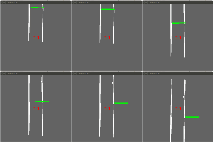
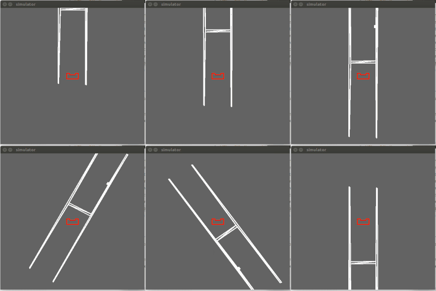
When at least 95% of all LRF points is smaller than a predefined range, detection passes the variable object the number that corresponds with a dead end.
This results in the activation of the dead end protocol. In this protocol Pico stops 0.4m in front of the dead end wall, beeps, and waits 5 seconds. After these 5 seconds, it looks if a door is opened or if it still is a dead end.
If object number still shows dead end, Pico turns 180 degrees and continues to drive. If a door was opened, Pico will continue the new path.
This is presented in the videos below.
 |
 |
Side door detection
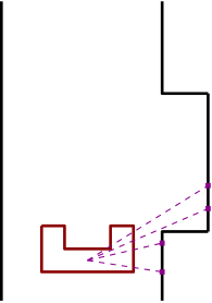
Because we use the limited LRF to place our reference points in open spaces, a side door is harder to detect. For these side doors a protocol was written to still detect these doors.<br\>
<br\>
When the robot drive through a corridor it keeps scanning a small set of points left and right for a sudden change in LRF range. When it detects a sudden change, the algorithm will check if the x values with reference to the robot lie within a certain tolerance. This was done respectively for the points after the sudden change and for the points before. This was done to make it more robust to ,for example, small gaps in a wall.
 |
 |
Limited range open-space detection
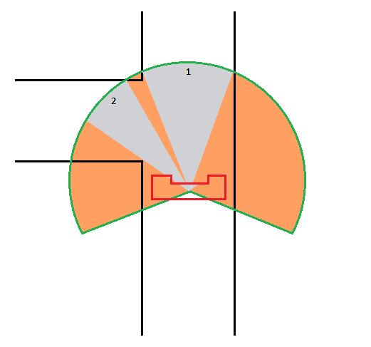
To detect possible corridors more robustly, a variable limited LRF range was used. By limiting the LRF range, possible open spaces which can indicate corridors can be detected, these can be seen in the figure below.
 |
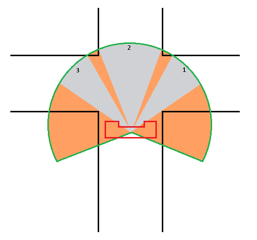 |
The pictures show the limited LRF range of Pico before a crossing. The grey area is where all the limited LRF points are equal to the set maximum range. The orange area is where the LRF data detects a point within the limited-LRF data.
The open space detection looks at all the limited range data in a loop from right to left anti-clockwise and determines when a high number of consecutive points are equal to the limited range.<br\> This area is an open space, thus a potential corridor. In the figure above this can be seen as the gray area. To prevent any small gaps to be detected, a minimum amount of conclusive points have to be detected in order to label it a potential corridor.
Each time a potential corridor is detected, an x and y reference in the middle of the potential corridor at maximum range is stored. The first one detected is always saved as the first reference, the second one detected as the second reference etc, moving from right to left.<br\> This is also indicated with the numbers in the open-spaces in the figure above.
When driving in an actual open-space, the maximum range of the LRF data is increased such that it can again detect potential corridors further away. The most right open-space is always the first reference, one open-space to the left the second etc. This can be seen in the figures above.
The source code can be found below in the section Code.
Localization
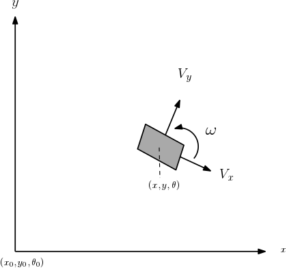
Being aware of the global position of the robot is critical for mapping and also useful for the motion of the robot. The global position of the robot is formulated as, [math]\displaystyle{ \begin{bmatrix}
x\\
y\\
\theta
\end{bmatrix} }[/math]. The figure below shows a graphical representation of the global position.
Discrete time model
With help of goniometric properties, the discrete time model of the global position of the robot is as follows,
[math]\displaystyle{ \begin{bmatrix} x_k\\ y_k\\ \theta_k \end{bmatrix} =\begin{bmatrix} x_{k-1}+V_x\Delta{t}\cos(\theta_k)-V_y\Delta{t}\sin(\theta_k) \\ y_{k-1}+V_x\Delta{t}\sin(\theta_k)+V_y\Delta{t}\cos(\theta_k) \\ \theta_{k-1}+\omega{\Delta{t}} \end{bmatrix} }[/math].
Where [math]\displaystyle{ V_x }[/math] is the sideward velocity, [math]\displaystyle{ V_y }[/math] the forward velocity, [math]\displaystyle{ \omega }[/math] the rotational speed and [math]\displaystyle{ \Delta{t} }[/math] the duration of each time step in the discrete model.
Extended Kalman filter
Since the odometry data is unreliable for a long run a Kalman filter is applied to minimize the error in the global position of the robot. The following is needed for a Kalman filter in context of the robot:
- Prediction model of the global position.
- Input data.
- Odometry data.
- Process noise and measurement noise.
The discrete time model of the global position that was mentioned before is being used as the prediction model for the global position. The input data are the forward speed, sideward speed and rotational speed calculated by the code and giving to io.sendBaseReference(). Combining the prediction model and the input data will give an estimation of the global position of the robot. To get a proper estimation of the global position, the measurement noise and the process noise need to be modelled correctly. The measurement noise can be based on sampling experimental data and deriving the statical properties. The covariance matrix [math]\displaystyle{ R }[/math] of the measurement noise can be calculated by,
[math]\displaystyle{ R_{ij} = \frac{1}{N-1}\sum_{k=1}^{N}(x_i-\bar{x}_i)(x_j-\bar{x}_j). }[/math].
The covariance matrix [math]\displaystyle{ Q }[/math] which represents the process noise is not as straightforward as the covariance matrix for the measurement noise. It is being used to filter the errors in the system model. Therefore the covariance matrix [math]\displaystyle{ Q }[/math] is being treated as a tuning parameter. A piece of the code that is used for the extended kalman filtering is shown below.
//=====================Prediction=========================
// State estimation
   x[2] = x_[2] + omega/freq;
   x[0] = x_[0] + Vx/freq*cos(x[2]) - Vy/freq*sin(x[2]);
   x[1] = x_[1] + Vx/freq*sin(x[2]) + Vy/freq*cos(x[2]);

   x_[0] = x[0];
   x_[1] = x[1];
   x_[2] = x[2];

// Covariance estimation
    P = J*P*transJ+Q;

//===================Updating=============================
// Measurement residual
   y[0] = deltaodomx-Vx/freq;
   y[1] = deltaodomy-Vy/freq;
   y[3] = deltaodoma-theta/freq;

// Innovation residual
    Mat S = H*P*transH+R;

// Kalman gain
    Mat K = P*transH*S.inv();

// Updated state estimation
    Mat xest = x+K*y;

// Updated covariance estimation
     P = (Mat::eye(3,3,CV_64F)-K*H)*P;
The extended Kalman filter follows the following scheme to estimate the global position of the robot.
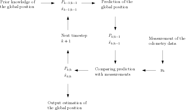
Unfortunately, the data collected from the experiments did not seem trustworthy, and there were no more opportunities to test these results. From there on a decision was made not to use the estimations calculated from the Kalman filter.
Mapping
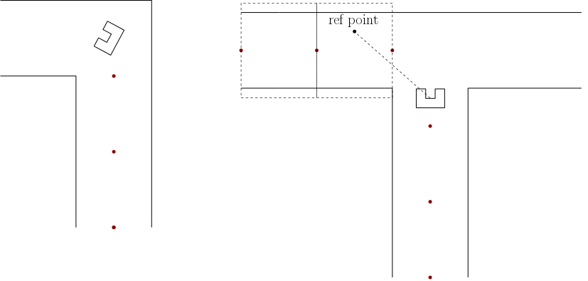
The idea of mapping is to memorize certain points in the maze. This would be used to solve the maze, as the code would tell whether the robot had already visited certain locations in the maze. The initial idea was to save the positions of landmarks of maze, in this case corners of the corridors and points that are used to recognize conjunctions. This has proven to have some difficulties. This is why a decision has been made to map the maze with another method. This method is pretty straightforward. Every two seconds during the maze solving it registers the current position of the robot, see the left picture for a graphical representation where the red dots represent the registered positions. These positions are saved in a list which are used in the maze solving algorithm.
In order to solve the maze, the locations the robots already visited need to be recognized. The recognition of visited locations is made possible by creating a virtual rectangular box between a saved position and its preceding saved position while it is being aligned with the corresponding corridor. The right figure above shows a graphical representation where virtual rectangular boxes are created between saved positions. So when a reference point is set in an area created by these boxes the code can recognize whether the location of the reference point had already been visited, this can contribute to the maze solving.
Planning
Here the planning is addressed. The 'planned' planning is the planning such as it was initially designed for implementation. Due to difficulties however, this planning was replaced by the 'final' planning.
The planned planning
The initial idea was the following. Detection gave the object ahead to planning. Planning had information about this object and previous object from mapping. Using this information, and the Tremaux's algorithm, planning placed a reference at a specific point. This system should have been able to solve the maze. However, difficulties in the implementation of mapping and object detection forced the group to develop an other strategy.
The final planning
The final decision making algorithm makes use of the limited range open-space detection. It creates a reference point at one of the open spaces. Initially, the preference is given to the right most open space. Following the right wall always ensures solving the maze, unless the robot starts in a loop. Therefore, another algorithm was developed that prevents the robot from staying in a loop. This algorithm is elaborated below.
Loop prevention<br\> The algorithm is based on the odometry data. An adjustment to the odometry data was made to make the data continuous, so without jumps. The planning block will have at most three potential reference points to chose from, right, middle or left. Initially Pico will always pick the first reference point, which will be the most right option. When Pico has turned a few times to the right, the planning block picks the second reference point when available. When Pico continues to turn to the right, planning will always pick the last reference point.<br\> So when the robot is in a loop by driving in a clockwise rotation, he will search eventually look voor a left corridor and pick this reference. <br\> If he keeps driving in an anti-clockwise rotation, he will look for an exit at the right after a few turns.
Below is a video of the robot using this algorithm to get out of of a loop.
 |
The maze challenge
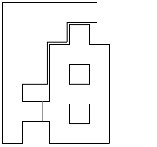
The maze from our maze challenge can be seen in the figure to the right.
The result
Unfortunately we didn’t pass the Maze challenge itself.
During the first attempt the robot recognized doors everywhere and the robot eventually collided sideways in a wall.
During the second attempt the robot turned right, took another right and then continued the corridor until it passed the door on the left and turned right again. Then Pico drove close to a wall, stopped and then bumped into it again.
Evaluation
During both attempts, the planning block interfered with the driving. The planning block chooses a reference point out of all possible choices based on how many rotations the robot has made. To estimate the number of rotations Pico has made, the odometry data was used. When Pico made more than around 1.5 rotation to the right (540 degrees in comparison to the start condition), the reference point switched from first reference point to second. Unfortunately the switching criterion between picking the first or second reference was determined mid-cornering due to the odometry data already having an initial state at the start. This caused the Robot to simultaneously switch between picking the first and second reference, which lead to the robot driving to the wall between the reference points.
On top of that, the potential field wasn’t scaled aggressively enough to prevent a side ways collision.
Fixing the problem
To fix the problem described above, the potential field was scaled a bit more agressively. Furthermore, reference choice was made more robust by introducing a state. <br\> If Pico made more than around 1.5 rotations to the right, a state was introduced that keeps picking the second reference point until the cumulative rotations of pico is zero again. <br\> When Pico makes more than around 2.5 rotation to the right, another state was introduced to keep picking the last reference point until the rotation decrease to 1.5. After falling below around 1.5 rotations, the second reference point is picked again.<br\> This is shown in the code below.<br\>
int corner=0;
float oneandhalfrot=-9;    // This is in radians and is a bit less than 1.5 rotations.
float twoandhalfrot=-16;   // This is in radians and is a bit more than 2.5 rotations.
float resetrot1=-1;        // This is a bit less than the starting condition.
float resetrot2=-10;

//Solving stategy for the maze. At first the robot will always take the most right reference point,
//however, when a certain amount of clockwise rotation is passed, it will take the second reference point, if available. After even
//more clockwise rotation the robot will take the last reference point available.

//below is the code to determine which reference point to pick at the next crossing.
if(odoma>0)
{
    cstate=0;                                               //state for which the most right reference point is preferred.
}                                                           //This is our choice making state.

if(odoma<oneandhalfrot && odoma>twoandhalfrot &&cstate==0)  //When this argument is satisfied the choice making state changes
{
    cstate=1;                                               //state for which the second reference point is preferred
}
if (odoma<twoandhalfrot&&cstate==1)                         //When this argument is satisfied the choice making state changes again.
{
    cstate=2;                                               //state for which the last reference point is preferred
}

if (cstate==1&& odoma>resetrot1)                            //When this argument is satisfied the choice making state resets to
{                                                           //the most right reference point again.
    cstate=0;
}
if (cstate==2&& odoma>resetrot2)                            //This argument resets the ref point preference from the last ref point to second.
{
    cstate=1;
}

//below is the code that couples the preferred reference point to the options that are available.
//A corner state of 0 means that the most right option is preferred, which is always available. This is
// each loop the inital state of corner. if the corner state is 1, it will directly pick the second reference point,
//and when it is 2 it will directly pick the third reference point.
//The difference between the choice making state and the corner state is that the choice state gives a preference, while
//the corner state is based onthe combination of the available options and the preferred state.
if (cstate==1)                                              //When the choice state state is 1, this argument check wether there are more than
{                                                           //one options available. If this is the case, it will pick the second ref point.
    if(data2.nrop>1)                                        //This state gives the actual number of options available.
    {
    corner=1;
    }
}
if (cstate==2)                                              // When the choice state is 2, this argument check wether there are more than
{                                                           //one options available. If there are two options, it will pick the second ref point,
    if(data2.nrop==2)                                       //and when there are 3 options, it will pick the third reference ref point.
    {
    corner=1;
    }
    else if(data2.nrop>2)
    {
    corner=2;
    }
}
<br\> Below is a video where Pico passes the Maze Challenge in the simulation. In this simulation Pico first turns right every corner, until it drives into his starting position again. Pico has rotated 1.5 times, so now it follows the second reference point until it rotates back until his starting orientation is reached. Now Pico starts picking the first reference point again.<br\> He then drives into a dead end to check for a door, turns around and pick the right corner again. After a while he detect the door on his right, turns into the the corridor, turns right again. After reaching the open space he adjusts his maximum range to still see the walls and drives to the end.
 |
Conclusion
Robustness is the key in unpredictable situations. Even though the robot successfully completed several test, during the maze challenge it bumped into a wall. Furthermore, thinking about the integration of individual pieces of code into the main software is critical for efficient programming. Design architecture and overall communication should be worked out before beginning the actual programming. Here are some more conclusions and experiences gathered:
- Overall C++ programming
- Working with GIT
- Avoid magic numbers for scalability of the code
- Simulations differ from the reality, therefore again robustness is required
- First create a solid basic to work from, then expand
- Clear and frequent communication between team members is critical for the progress of the group
Recommendations
Due to a restart of the project and the limited manpower, there are certain elements we could not spend (enough) time on. The following would have been implemented or considered if there was time to improve the quality of the solution to the maze solving problem.
- As mentioned before, the extended Kalman filter lacks a proper covariance matrix for the measurement noise due to dubious measurement data which could not be tested. A proper testing plan should have been created and the results from the testing should be evaluated by other tests. This would result in an extended Kalman filter of a higher quality.
- There were problems with mapping where it did not tell if the location was already visited when it should. Visualisation of the mapping should be implemented. This could be a great asset in terms of debugging.
- Making side door detection more robust. Sometimes the robot didn't recognize doors because our requirements were too strict.
Code
Files
- Initial design: Initial idea report
- Intermediate presentation: Intermediate presentation
- Final presentation: Final presentation