Embedded Motion Control 2016 Group 7: Difference between revisions
| (75 intermediate revisions by 4 users not shown) | |||
| Line 162: | Line 162: | ||
== '''Movement''' == | == '''Movement''' == | ||
--> | --> | ||
| Line 240: | Line 202: | ||
In this state the robot will get once things have gone wrong. All the mapping will be deleted. Next a new fit will be made and a new setpoint will be determined. If the fit is unreliable or there cannot be created a setpoint, the robot will turn 0.5 radians and try again until it has succeeded to get a reliable fit and a setpoint. Once a setpoint is determined, the state will change to the driving state. | In this state the robot will get once things have gone wrong. All the mapping will be deleted. Next a new fit will be made and a new setpoint will be determined. If the fit is unreliable or there cannot be created a setpoint, the robot will turn 0.5 radians and try again until it has succeeded to get a reliable fit and a setpoint. Once a setpoint is determined, the state will change to the driving state. | ||
= '''Environment identification''' = | |||
Below is a code snippit including the first two states of the coordinator. | |||
switch (state) | |||
{ | |||
//1 Setpoint achieved | |||
case 1: | |||
{ | |||
// Make new fit | |||
preprocess(scan); | |||
area_optimization_algoritm(frontsight,0,false); | |||
if (fit_reliable) | |||
{ | |||
// Recognize nodes locally and convert to global coordinates | |||
local_node_recognition(dv_center, side_road, relativeDirections, localcorrx, localcorry); | |||
scatter_local_nodes(relativeDirections); //Matlab scatter output for local directions for debugging | |||
// Calculate odometry correction using local nodes | |||
Odometry_correction(dv_center, orientationpico,localcorrx,localcorry,angle_deviation,correction_x,correction_y); | |||
// Update global odometry with correction | |||
updatepicoodom(odom.x,odom.y,odom.a); | |||
// Save local nodes in mapping | |||
globalmapping(globalDirections, relativeDirections, crossingSides, visibleDirections); | |||
} | |||
else | |||
{ | |||
// If fit not reliable, go to state for small driving for new fit | |||
state=4; | |||
dv_center(0)=0; | |||
} | |||
// List all setpoints of mapping in output, also scatter of setpoints, for debugging | |||
listAllGlobalDirections(globalDirections,visibleDirections); | |||
// Determine which setpoint to go to next | |||
Mazesolver(x,y,a); | |||
if (no_setpoint) | |||
{ | |||
// Go to state for small driving for new fit | |||
state=4; | |||
no_setpoint=false; | |||
} | |||
else //All good | |||
{ | |||
// Go to driving state | |||
state = 2; | |||
} | |||
break; | |||
} | |||
//2 Drive to setpoint | |||
case 2: | |||
{ | |||
// If dead end is recognized by mazesolver | |||
if (dead_end) | |||
{ | |||
// Go to Possible door state | |||
state = 3; | |||
dead_end=false; | |||
} | |||
// If setpoint is reached | |||
else if((sqrt(square(pico_x-x)+square(pico_y-y)) < marginxy) && (fabs(fmod(((pico_a)-(a)),2*3.13)) < margina)) | |||
{ | |||
// Put velocity zero to prohibit driving while optimizing rectangles | |||
io.sendBaseReference(0,0,0); | |||
// Go to setpoint achieved state | |||
state = 1; | |||
} | |||
// If no dead end nor setpoint reached, drive to setpoint | |||
else | |||
{ | |||
// Determine drive inputs | |||
Potential_field(scan,x,y,a,vx,vy,va,exitflag); | |||
// If the resulting force is backwards | |||
if(exitflag == 5) | |||
{ | |||
// If the setpoint is near, set the setpoint as achieved and determine new setpoint | |||
if ((sqrt(square(pico_x-x)+square(pico_y-y)) < marginxy+0.3))// ||exitflag==1 | |||
{ | |||
// Determine new setpoint | |||
Mazesolver(x,y,a); | |||
// Determine drive inputs | |||
Potential_field(scan,x,y,a,vx,vy,va,exitflag); | |||
} | |||
else | |||
{ | |||
// If setpoint is not close, try to find a new setpoint | |||
no_setpoint = true; | |||
} | |||
if (no_setpoint) | |||
{ | |||
// Go to state for small driving for new fit | |||
state=4; | |||
no_setpoint=false; | |||
} | |||
else // All good, drive to new setpoint | |||
{ | |||
state = 2; | |||
} | |||
} | |||
// If stuck | |||
else if(exitflag == 2 && fabs(va) < 0.1){ | |||
// Go to stuck state | |||
state = 6; | |||
} | |||
else | |||
{ | |||
// Execute driving | |||
io.sendBaseReference(vx,vy,va); | |||
} | |||
} | |||
break; | |||
} | |||
//3 Possible door | |||
case 3: | |||
{ | |||
} | |||
case 6: // stuck | |||
{ | |||
} | |||
case 7: // Stuck driving | |||
{ | |||
} | |||
case 99: // Reset | |||
{ | |||
} | |||
} | |||
== '''Environment identification''' == | |||
To subtract relevant information from the laser data an environment identification algorithm is used. This algorithm determines the dimensions of the corridor where pico is positioned, and it determines all the position and location of the visible sideroads. Using this information the world model can be updated, and the odometry data can be corrected. | To subtract relevant information from the laser data an environment identification algorithm is used. This algorithm determines the dimensions of the corridor where pico is positioned, and it determines all the position and location of the visible sideroads. Using this information the world model can be updated, and the odometry data can be corrected. | ||
== '''General model''' == | === '''General model''' === | ||
To be able to identify the environment a general model is proposed as shown in the figure to the right. The model consist of the current corridor, the corridor Pico is placed at the moment of the identification, and side roads at the west, north and east side of this current corridor. | To be able to identify the environment a general model is proposed as shown in the figure to the right. The model consist of the current corridor, the corridor Pico is placed at the moment of the identification, and side roads at the west, north and east side of this current corridor. | ||
The general model is parameterized relative to Pico. So the angle the current corridor as relative to Pico is described by \theta. The distance to the West and East walls are described with A and B respectively. To distance to the North and South are described with l and m respectively. | The general model is parameterized relative to Pico. So the angle the current corridor as relative to Pico is described by <math>\theta</math>. The distance to the West and East walls are described with <math>A</math> and <math>B</math> respectively. To distance to the North and South are described with <math>l</math> and <math>m</math> respectively. | ||
It is assumed that all the corridors are perpendicular to each other. Hence, each side road can be described with 3 parameters, the width (C), the length (D) and the location with respect to the current corridor. | It is assumed that all the corridors are perpendicular to each other. Hence, each side road can be described with 3 parameters, the width (<math>C</math>), the length (<math>D</math>) and the location with respect to the current corridor (<math>e</math>). It is possible to detect a side road on the West, North, and East side of the current corridor, these are each identified with the numbers 0, 1 and 2 respectively. Because the LRF can not detect points behind Pico it is impossible to detect a side road on the South side of the current corridor. | ||
The open spaces can be interpreted as a wide side road, which means a possible side road in an open space should be to overlap with the ‘side road’ connected to the open space. | The open spaces can be interpreted as a wide side road, which means a possible side road in an open space should be to overlap with the ‘side road’ connected to the open space. | ||
| Line 255: | Line 342: | ||
[[File:general_model.png|upright=2.5|General model of local environment]] | [[File:general_model.png|upright=2.5|General model of local environment]] | ||
== '''Algorithm''' == | === '''Algorithm''' === | ||
The general algorithm consists out of the following steps | The general algorithm consists out of the following steps | ||
# Preprocess laser data | # Preprocess laser data | ||
| Line 261: | Line 348: | ||
# Determine location and dimension of side roads | # Determine location and dimension of side roads | ||
# Determine reliability of the found dimensions | # Determine reliability of the found dimensions | ||
=== ''' Preprocess laser data '''=== | ==== ''' Preprocess laser data '''==== | ||
[[File:Emc2016_group7_Preprocess.png|thumb|right|upright=2|Laser data after preprocessing]] | |||
First the laser data is preprocessed. The characteristics of the LRF are that in large gaps between points ‘Ghost Points’ occur. First these Ghost Points are filtered out on the basis that there are no points close to these points. Furthermore the algorithm does not need all the points from the laser data, therefore the points can be filtered such that a set of points that are really close to each other can be combined into 1 point. Using this only relevant points remain and the computation time of the algorithm increases. | First the laser data is preprocessed. The characteristics of the LRF are that in large gaps between points ‘Ghost Points’ occur. First these Ghost Points are filtered out on the basis that there are no points close to these points. Furthermore the algorithm does not need all the points from the laser data, therefore the points can be filtered such that a set of points that are really close to each other can be combined into 1 point. Using this only relevant points remain and the computation time of the algorithm increases. | ||
=== ''' Determine current corridor ''' === | ==== ''' Determine current corridor ''' ==== | ||
[[File:Emc2016_group7_Current_Corridor.png|thumb|right|upright=2|Found current corridor in laser data]] | |||
Using the relevant data the dimensions of the current corridor are determined. This is done by maximizing the area of this corridor, with the LDR data as boundary. | Using the relevant data the dimensions of the current corridor are determined. This is done by maximizing the area of this corridor, with the LDR data as boundary. | ||
==== ''' Optimization problem formulation ''' ==== | ===== ''' Optimization problem formulation ''' ===== | ||
The optimization problem can be formulated as | The optimization problem can be formulated as | ||
: <math>\begin{align} | : <math>\begin{align} | ||
| Line 283: | Line 372: | ||
The upper and lower bound for the design variables are chosen such that the dimensions of the rectangle stay realistic. It is assumed that Pico is positioned almost straight in the current corridor at the moment of the identification, therefore small upper and lower bounds are used for <math>\theta</math> | The upper and lower bound for the design variables are chosen such that the dimensions of the rectangle stay realistic. It is assumed that Pico is positioned almost straight in the current corridor at the moment of the identification, therefore small upper and lower bounds are used for <math>\theta</math> | ||
==== ''' Initial conditions ''' ==== | ===== ''' Initial conditions ''' ===== | ||
From the optimization the best results are obtained when starting with feasible initial conditions. It is assumed that Pico is standing straight in the main corridor, therefore the initial condition for <math>\theta=0</math>. The initial conditions for <math>A</math> and <math>B</math> are half the length of Pico, corresponding to the smallest corridor possible. The initial condition for <math>m</math> is also chosen small, but for the initial condition of <math>l</math> the LFR data in front of Pico is used. This is done because otherwise the rectangle is able to rotate in the beginning phases of the optimization, which will lead to a higher chance of a local minima. | From the optimization the best results are obtained when starting with feasible initial conditions. It is assumed that Pico is standing straight in the main corridor, therefore the initial condition for <math>\theta=0</math>. The initial conditions for <math>A</math> and <math>B</math> are half the length of Pico, corresponding to the smallest corridor possible. The initial condition for <math>m</math> is also chosen small, but for the initial condition of <math>l</math> the LFR data in front of Pico is used. This is done because otherwise the rectangle is able to rotate in the beginning phases of the optimization, which will lead to a higher chance of a local minima. | ||
=== ''' Determine side roads ''' === | ==== ''' Determine side roads ''' ==== | ||
[[File:Emc2016_group7_Expected_Points.png|thumb|right|upright=2|Expected and deviating points of the current corridor]] | |||
[[File:Emc2016_group7_Side_Roads.png|thumb|right|upright=2|Found side roads]] | |||
Next all the locations and dimensions of the side roads are determined. Again this is formulated as maximizing the area of a side road, with the LDR data as boundary. | Next all the locations and dimensions of the side roads are determined. Again this is formulated as maximizing the area of a side road, with the LDR data as boundary. | ||
==== ''' Optimization problem formulation ''' ==== | ===== ''' Optimization problem formulation ''' ===== | ||
the optimization problem can be formulated as | the optimization problem can be formulated as | ||
: <math>\begin{align} | : <math>\begin{align} | ||
&\underset{x}{\operatorname{maximize}}& & f(x)=C\cdot D \\ | &\underset{x}{\operatorname{maximize}}& & f(x)=C\cdot D=x_1\cdot x_2 \\ | ||
&\operatorname{subject\;to} | &\operatorname{subject\;to} | ||
& & e_i(x) \leq 0, \quad i = 1,\dots,n \\ | & & e_i(x) \leq 0, \quad i = 1,\dots,n \\ | ||
| Line 298: | Line 389: | ||
\end{align}</math> | \end{align}</math> | ||
where | where | ||
* <math>x_0=e</math>, <math>x_1=C</math>, <math>x_2=D</math> | |||
* the objective function <math>f(x)</math> is defined by the area of the rectangle, | * the objective function <math>f(x)</math> is defined by the area of the rectangle, | ||
* <math>e_i(x)</math>the smallest distance of point <math>i</math> to the sides of the rectangle, hereby the error is positive if the point is inside the rectangle, and | * <math>e_i(x)</math>the smallest distance of point <math>i</math> to the sides of the rectangle, hereby the error is positive if the point is inside the rectangle, and | ||
* <math>n</math> are the number of points. | * <math>n</math> are the number of points. | ||
==== ''' Initial conditions ''' ==== | ===== ''' Initial conditions ''' ===== | ||
To find all side roads is a bit hard, because each side road represents a local minima in the optimization problem. It is therefore necessary to have a good guess what the location of the side road is. To obtain this good initial conditions the results from the current corridor are used. Using the dimensions of this corridor the expected LRF data without side roads can be determined. At the locations where no side road is present this expected LRF data should be close to the expected LRF data. At the locations of the side roads the expected LRF data deviates from the real LRF data, using this the initial conditions for the location and width of the side road are determined. The initial length of the side road is the minimal depth of a door to be able to detect a door, which is in fact a side road with a small length. | |||
=== ''' Determine reliability ''' === | ==== ''' Determine reliability ''' ==== | ||
Although the algorithm is fairly robust, in some situations it does not provide a sufficient solution. Because it is unwanted that these identifications are used in for the global mapping and odometery correction it is necessary to determine if the result is reliable. | |||
To do this the estimated points used for the initial conditions are used again. The reliability is determined by comparing all the estimated LFR data to the real LRF data. All the estimated points which corresponds to points inside a found side road are not taken into account. | |||
= '''Mapping''' = | === '''Implementation using dlib''' === | ||
The optimization problems in the algorithm are solved using the c++ library [http://dlib.net/ dlib]. In this library an optimization toolbox is present. This toolbox is able to solve unconstrained optimization problems without the knowledge of the gradient of the objective function using BFGS algorithm. When an objective function is present this toolbox provides a fairly simple manner to maximize this objective function: | |||
find_max_using_approximate_derivatives(bfgs_search_strategy(), | |||
objective_delta_stop_strategy(1e-5), | |||
objfun_center, dv_center, 1000, 1e-5); | |||
Note that the optimization problems in the algorithm are constrained optimization problems. To cope with this the problem formulation is transformed to an unconstrained optimization problem by applying the constraints as exterior penalty functions on the objective function. | |||
// Original objective function | |||
double f=(A+B)*(m+l); | |||
// Penalty for error on points | |||
for (int i=0; i<n; i++) | |||
{ | |||
f-=n/r_point*pow(error(i),4); | |||
} | |||
// Penalty for bounds | |||
for (int i=0; i<5; i++) | |||
{ | |||
f-=1/r_bound*pow(max(-dv_center(i)+dv_center_lb(i), 0.0),2); | |||
f-=1/r_bound*pow(max(dv_center(i)-dv_center_ub(i), 0.0),2); | |||
} | |||
== '''Mapping''' == | |||
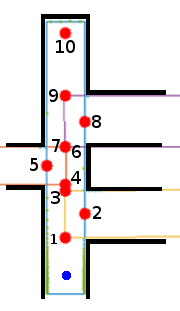
[[File:Emc2016_group7_localnodes.png|thumb|right|Local direction recognition, red points are directions, blue point is actual PICO position, colored rectangles are optimization results, black outline are the real walls]] | [[File:Emc2016_group7_localnodes.png|thumb|right|Local direction recognition, red points are directions, blue point is actual PICO position, colored rectangles are optimization results, black outline are the real walls]] | ||
In the environment identification the current corridor and side roads are found relative to PICO. This can be translated to directions relative to PICO and positioning error relative to PICO. This is calculated in Local direction recognition. With the current location and orientation of PICO the directions relative to PICO can be rewritten to global directions from the origin. | In the environment identification the current corridor and side roads are found relative to PICO. This can be translated to directions relative to PICO and positioning error relative to PICO. This is calculated in Local direction recognition. With the current location and orientation of PICO the directions relative to PICO can be rewritten to global directions from the origin. | ||
The mapping is build on the fact that the maze consists of crossings and turns. Each crossing consists of directions pointing away from the crossing. As the maze is axis aligned, all directions point either North, West, South or East. A crossing can thus be represented by multiple directions, which belong to the same intersection. A corner can be represented by two directions belonging to the same intersection, and a dead end by a single direction belonging to a intersection. | The mapping is build on the fact that the maze consists of crossings and turns. Each crossing consists of directions pointing away from the crossing. As the maze is axis aligned, all directions point either North, West, South or East. A crossing can thus be represented by multiple directions, which belong to the same intersection. A corner can be represented by two directions belonging to the same intersection, and a dead end by a single direction belonging to a intersection. | ||
In order to connect crossings, corners and dead ends the directions have to be connected. Hence the maze is represented by nodes(intersections) and edges(connected nodes) which in turn results in a undirected graph. In order to store the maze the position, orientation, intersection (number), connected direction are saved for each node together with the direction ID (which is used also for the connected direction) and the number of times that direction has been passed(which is used in the Maze solving algorithm later). | In order to connect crossings, corners and dead ends the directions have to be connected. Hence the maze is represented by nodes(intersections) and edges(connected nodes) which in turn results in a undirected graph. In order to store the maze the position, orientation, intersection (number), connected direction are saved for each node together with the direction ID (which is used also for the connected direction) and the number of times that direction has been passed(which is used in the Maze solving algorithm later). | ||
== '''Local direction recognition''' == | === '''Local direction recognition''' === | ||
| Line 327: | Line 444: | ||
Depending on whether the local direction recognition is called in a crossing or in a corridor it calculates the position of the end or the beginning of the first crossing. As this function is only called when a setpoint is reached this is a method to verify if PICO is on that setpoint. That location is later used to correct the odometry data. | Depending on whether the local direction recognition is called in a crossing or in a corridor it calculates the position of the end or the beginning of the first crossing. As this function is only called when a setpoint is reached this is a method to verify if PICO is on that setpoint. That location is later used to correct the odometry data. | ||
== '''Global mapping''' == | |||
<br> <br> | |||
=== '''Global mapping''' === | |||
[[File:Emc2016_group7_gm2.png|thumb|300px|right|Global mapping visualized in maze design of 2016. The blue point is where PICO starts, the black points is the path PICO has driven, the red points is the mapping]] | [[File:Emc2016_group7_gm2.png|thumb|300px|right|Global mapping visualized in maze design of 2016. The blue point is where PICO starts, the black points is the path PICO has driven, the red points is the mapping]] | ||
[[File:Emc2016_group7_gm1.png|thumb|300px|left|Global mapping visualized in maze design of 2015. The blue point is where PICO starts, the black points is the path PICO has driven, the red points is the mapping]] | [[File:Emc2016_group7_gm1.png|thumb|300px|left|Global mapping visualized in maze design of 2015. The blue point is where PICO starts, the black points is the path PICO has driven, the red points is the mapping]] | ||
| Line 342: | Line 462: | ||
The result of the global mapping is visualized on the left and right for the maze design of 2015 and 2016. What can be seen on the left(2015) is that the mapping correctly detects directions, even for crossings that PICO has not visited yet but has seen already. In the maze on the right(2016) the green boxed intersection is an example of an intersection where (seen from the left) the right corridor starts before the left road has ended. Which is why this is considered as 1 intersection instead of 2 separate ones. Before the end of the maze there is a direction (boxed in purple) which should not be there, but is seen because of the corner in the open space. In this case it would not be a problem. If PICO ware to pick that direction, and scan the environment again it would still drive out to the final direction and drive out of the maze(this is the case in the third simulation of this years maze design below). | The result of the global mapping is visualized on the left and right for the maze design of 2015 and 2016. What can be seen on the left(2015) is that the mapping correctly detects directions, even for crossings that PICO has not visited yet but has seen already. In the maze on the right(2016) the green boxed intersection is an example of an intersection where (seen from the left) the right corridor starts before the left road has ended. Which is why this is considered as 1 intersection instead of 2 separate ones. Before the end of the maze there is a direction (boxed in purple) which should not be there, but is seen because of the corner in the open space. In this case it would not be a problem. If PICO ware to pick that direction, and scan the environment again it would still drive out to the final direction and drive out of the maze(this is the case in the third simulation of this years maze design below). | ||
== '''Odometry correction''' == | |||
[[File:Emc2016_group7_odometry_angle.png|thumb|300px|right|Graphical representation of orientation correction of Pico at two setpoints <math>A</math> and <math>B</math>]] | |||
Due to slip that the Pico has in the real world, it is crucial that there is correct odometry correction. In total three corrections are introduced: the rotation, the absolute x-direction and y-direction. This is devided in two parts. Firstly, the angle correction is explained. Subsequently, the correction for the x- and y-direction is enlightened. Note that for both corrections the rectangle fits are used. Since the rectangle fit was already implemented, it would be cumbersome to not use it. Furthermore, the location of Pico has not to be precise since an accuracy of 5 cm is not an issue. Therefore, in our opinion Kalmann is a little bit of overkill. | |||
=== '''Correction for orientation odometry''' === | |||
In the environment identification, rectangles are fitted which can be used to correction the angle diviation of Pico with respect to the main current corridor. As mentioned above, one of the design variables of the current corridor is the angle <math>\theta_{laser}</math> which is the offset off Pico. At each setpoint, a new rectangle fit is constructed. Since the direction of the setpoint is either forward, backwards, to the right, or to the left, it can be constructed what the desired odometry data should be denoted by <math>\theta_{setp}</math>. Furthermore, the real Pico orientation is known denoted by <math>\theta_{real}</math>. Subsequently, at each setpoint, when the rectangle fit is reliable, the following intuitive Equation is used to calculate the offset: | |||
<math>theta_{deviation} = \theta_{real} - theta_{setp} - theta_{laser} </math> | |||
The figure to the right is a graphical representation of this correction. Note that at each setpoint the orientation of the Pico is corrected. The final deviation of the angle is used to correct the global pico orientation odometry. Both in the simulation and during experiments this correction it was found that this correction was implemented succesfull and usefull. | |||
=== '''Correction for x- and y-direction odometry''' === | |||
[[File:Emc2016_group7_odometry_x_y_direction.png|thumb|300px|left|Graphical representation of x-, and y-direction correction of Pico at setpoint]] | |||
The concept for the x- and y-cirection was relatively simple. The desired setpoint was extracted from the Mazesolver given in x- and y-direction expressed with respect to the global coordinate frame noted by <math>x_{exp}</math> and <math>y_{exp}</math>. When a setpoint was reached, the function odometry correction was started. From the rectangle optimisation, it was able to locate the setpoint with respect from Pico in the local coordinate frame. These local coordinates, are transformed to the global coordinate frame using the following rotation matrix: | |||
:<math>R = | |||
\begin{bmatrix} | |||
\cos \theta & -\sin \theta \\ | |||
\sin \theta & \cos \theta \\ | |||
\end{bmatrix} | |||
</math> | |||
resulting in <math>\epsilon_x</math> and <math>\epsilon_y</math>. | |||
Since all distances are know expressed in the same global coordinate frame, the following Equations are used to determine the x- and y-deviation: | |||
:<math> | |||
x_{cor} = x_{exp} - \epsilon_x - x_{real} </math> | |||
:<math> | |||
y_{cor} = y_{exp} - \epsilon_y - y_{real} </math> | |||
In the end, these corrections are applied in the global coordinate frame. However, it appeared that the applied method did not result in the expected results. The main problem was that the accuracy of the local distance from Pico to the desired setpoint was not determined correctly. Due to this reason, Pico was corrected with unreliable data. Therefore, the functioning of the mapping was bad. The second reason why this implementation of the odometry correction for x- and y-direction was not ideal, is due to the update frequency. During the simulations it appeared that the odometry correction in x- and y-direction was not bothersome, nor did it actually help. Therefore, it is suggested as a recommendation to implement another method for the odometry correction. | |||
= '''Mazesolver''' = | == '''Mazesolver''' == | ||
The mazesolver makes use of the nodes which are created in the mapping. The coordinator decides when the mazesolver is ran. When the mazesolver runs it first checks if Pico is in a corridor or on an intersection. If Pico is in a corridor it looks in the list of known nodes and checks if there exists a node that is connected to the current node. If so the mazesolver will return the position of this node. Else the mazesolver will tell the coordinator that there is no connected node (the coordinator will then drive forward and try to find new nodes again). The mazesolver makes use of the Trémaux’s algorithm, when Pico reaches a node it will update the number of times Pico passed that node and it will always select the path where Pico has been the least. A dead-end is marked by updating the number of passes to 5, this way Pico will only try a dead-end once. | The mazesolver makes use of the nodes which are created in the mapping. The coordinator decides when the mazesolver is ran. When the mazesolver runs it first checks if Pico is in a corridor or on an intersection. If Pico is in a corridor it looks in the list of known nodes and checks if there exists a node that is connected to the current node. If so the mazesolver will return the position of this node. Else the mazesolver will tell the coordinator that there is no connected node (the coordinator will then drive forward and try to find new nodes again). The mazesolver makes use of the Trémaux’s algorithm, when Pico reaches a node it will update the number of times Pico passed that node and it will always select the path where Pico has been the least. A dead-end is marked by updating the number of passes to 5, this way Pico will only try a dead-end once. | ||
| Line 355: | Line 514: | ||
[[File:Mazesolver.PNG|400px|alt=The number of passes is shown at each node.|The number of passes is shown at each node.]] | [[File:Mazesolver.PNG|400px|alt=The number of passes is shown at each node.|The number of passes is shown at each node.]] | ||
= ''' | == '''Potential field''' == | ||
One of the key elements of this project, is that Pico should be able to drive autonomously. From a higher level, the software receives a setpoint in absolute coordinates with respect to the starting position of the robot. With this information, the robot can move towards this location. However, it should also be avoided to collide into the walls. Therefore, a potential field is implemented which is a relatively easy method. The key elements are the following two forces: | |||
:* <math>F_{repp}</math>: Repelling force to ensure the robot will not collide with the walls | |||
:* <math>F_{attr}</math>: Attracting force responsible for the movement towards the setpoint | |||
The potential field is a method from where the laser data range and angle with respect to the orientation of Pico are used. The wall forces will push Pico away from the walls, while the setpoint will attract Pico, see the Figure. | |||
[[File:Wall_vectors.png|right|200px|alt=Wall force vectors.|Wall force vectors exerted on Pico ]] | |||
On | For every laser range and angle, the following Equation is executed to calculate the force vector of that data point: | ||
<math>F_{repp,i} = \frac{1}{1375r_i^3 - 232.5r_i^2 + 12.19r_i} </math> | |||
[[File:Total_force.png|right|200px|Schematic representation of total force on Pico together with angle <math>\phi</math>]] | |||
where the three constants of the polynomial expression are used to optimize the repelling force vectors. Afterwards, the contribution in the x- and y-direction can be computed with help of the angle for each laser data. The attracting force is computed by the following Equation: | |||
<math>F_{attr} = e_x^2 + e_y^2</math> | |||
in where <math>e_x</math> and <math>e_y</math> are the relative error between Pico and the setpoint in meters. Afterwards, this force is normalised to ensure that <math>F_{attr}</math> will not go to zero when Pico is almost at the desired setpoint. Note that <math>F_{attr}</math> is with respect to the base coordinate frame. Since <math>F_{rep}</math> is in the relative coordinate frame, <math>F_{attr}</math> is rewritten to relative coordinates with a rotation matrix as used earlier in odometry correction. | |||
The parameters above are scaled in such a way that the following desired behaviour is exacted: | |||
:* When Pico is located close to a wall, <math>F_{rep} >> F_{attr}</math> | |||
:* When Pico is not located at a close distance to a wall, <math>F_{rep} << F_{attr}</math> | |||
Subsequently, the total force <math>F_{tot}</math> is calculated. From here, an angle <math>\phi</math> is obtained which can be used to calculate the desired velocities in the x- and y-direction, see the Figure. | |||
Afterwards, the velocity in x- and y-direction of the Pico is calculated by | |||
:<math> | |||
v_{x} = \text{cos}(\phi)v_{max}</math> | |||
and | |||
:<math> | |||
v_{y} = \text{sin}(\phi)v_{max}</math>. | |||
Additionally, when the total force angle is behind Pico, Pico will first start turning around before driving to the setpoint, to prevent Pico from driving backwards. This is dangerous due to the fact there is no laser data available at the back of Pico. For the rotational velocity, the error between the setpoint orientation and Pico's current rotation is used. | |||
== '''Solved problems''' == | |||
Once a week a experimental session was planned to test the written code. This usually introduced problems because of situations that ware not thought of, or because of uncertainties in the real world. A number of these problems are described below, as well as the solutions that ware implemented to solve these problems | |||
* Robot does not reset the odometry data when a new piece of code is executed. A initialization function was created that saves the initial position and rotation(the initial odometry data). Each new odometry data is then compared to the initial odometry data to obtain the corrected odometry. | |||
* Number of laser data points is not equal to 1000 as suggested in the simulator. Therefore, the values of minimum angle and maximum angle differ. Additionally, when there is a laser data point from where no object is visible, the laser data becomes infinity resulting in problems in the Potential field. These problems were found during the experiments and fixed in that week. | |||
* The local direction detection only checked the first intersection it saw in front of PICO. For the odometry correction a direction is needed that could also lie behind PICO. Therefore the local direction recognition is rewritten to detect all crossings it can see, such that all information that PICO has would be processed in the mapping and directions behind PICO could also be used for correction. | |||
* When PICO is at the start of a small corridor, and sees a side road on either side behind itself, a local direction would be detected for this side road. However when the laser data ends before the side road ends, the width of the side road would not be correct, and also the direction would be faulty, resulting in a non existent direction. During area recognition it can be seen that these side roads start as soon as the laser data starts. For each of these side roads it is passed along to the local direction recognition whether this is the case or not. The side roads that have this are not processed in the mapping, but could be processed for correction, since the end of the side road(closest to pico) is detected correctly. | |||
* Because the odometry correction did not work as well as hoped some errors occurred in the mapping. One of these errors is that local directions are not matched to a global direction, while they should be while others are. For example when the local direction(A) should be recognized as an already existing global direction but isn't. However when the connected local direction(B) is recognized as a global direction the first local direction (A) will not be connected while it should. This is an indication that local direction (A) is a faulty direction. Therefore direction A is removed from the mapping, as other directions that should be connected but aren't. | |||
= '''Simulations and attempts''' = | |||
== ''' Corridor challenge simulation''' == | |||
As can be seen in the video below the robot is able to do the corridor challenge. The robot follows two setpoints that are placed on the intersection edges. The setpoints are made using the rectangle fit and driving is done using the potential field. | |||
[[File:Emc2016_group7_corridorsim2.gif]] | |||
== ''' Corridor challenge attempt''' == | |||
During the real corridor challenge the robot behaved as expected. Our code used the same speed or cornering, as for straight paths. Since there ware some issues with PICO doing corners fast, the speed was lowered. This meant however, since the corridor was very long, that the time was not very fast: the robot could have driven faster on the straight. This is something that might be implemented for the maze challenge. We did get a nice compliment about the smooth cornering though! A link to the video of the corridor challenge is shown below. | |||
https://www.youtube.com/watch?v=upn1WE3GwSs | |||
== ''' Maze simulations''' == | |||
To prepare for the maze challenge multiple mazes ware created by hand, but the best test is that of the maze design of 2015. Which are are shown below. In the both simulations the maze solver chooses the direction on the crossing based on the number of passes of the directions. It picks the direction with the least passes. If the number of passes are equal the simulation on the left has a preference for left, then right, then straight, the simulation on the right picks one of the least passed direction at random. In both cases the maze is solved. In the situation on the right one can see the Tremaux algorithm picking visiting all the directions before picking the direction that leads to the door. No direction is passed more than 3 times. Both simulations are sped up with 150%. | |||
[[File:Emc2016_group7_maze20151.gif]][[File:Emc2016_group7_maze20152.gif]] | |||
== ''' Maze challenge attempts''' == | |||
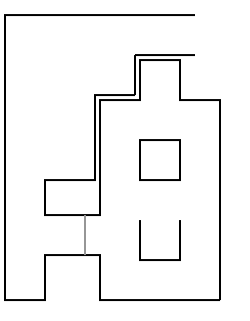
On June 8th 2016, the final Maze challange was held at the RoboCup soccer field. In total, 7 groups implemented their code on PICO to see which group was able to finish the maze. Each group had two attempts at solving the maze. The maze is depicted below and as one can see consists of multiple dead-ends, one loop, a rather tricky placed door, and an open-space. The starting position was the U-shaped corridor in the bottom of the figure. The open-space was located behind the door. At the end of the open-space, the exit was located. Below, the two attempts are discussed together with the results and a video of the challanges. | |||
[[File:maze_design_final_challange.png]] | [[File:maze_design_final_challange.png]] | ||
| Line 379: | Line 607: | ||
== '''Simulation''' == | == '''Simulation''' == | ||
After the maze challenge the maze design is used in the simulator to run the algorithm. For the simulations the maze solver was run on the setting that picks the least used direction. If there are multiple least used directions, then it picks one of these at random. Because of this the maze should be solved with different paths which can be seen below. For this the odometry correction is disabled, since in the simulator the odometry data corresponds with the actual position and rotation. Below each animation there is commentary. | After the maze challenge the maze design is used in the simulator to run the algorithm. For the simulations the maze solver was run on the setting that picks the least used direction. If there are multiple least used directions, then it picks one of these at random. Because of this the maze should be solved with different paths which can be seen below. For this the odometry correction is disabled, since in the simulator the odometry data corresponds with the actual position and rotation. Below each animation there is commentary. All three simulations are sped up with 150%. | ||
[[File: | |||
[[File:Emc2016_group7_final3.gif|400px|right|thumb|PICO goes left*, right*, right, straight*, right, straight*, right, right (then comes back at the intersection with the door). At this point PICO knows it is at that intersection and that it has been at all direction of the intersection once except for the door. Hence it goes trough the door. After the door it goes right* into the corridor that ends up as an open space. At the start of this corridor PICO drives forward, then idles for an instant, and repeats this a few times. In this moment PICO has not seen a new direction yet, as it is too far away, thus it drives forward. When it sees a new intersection it connects that direction to the last direction. It then drives to the middle of the open space, as it thinks the intersection right starts there. After that it goes right*, towards the direction that is not right in front of the exit. This would be the purple boxed direction described in the mapping. It then scans again, and sees the exit and drives towards it. | |||
The directions listed with an * are the directions that are not the only direction at that intersection with the least passings, and thus could have also been an other least passed direction.]] | |||
[[File:Emc2016_group7_final1.gif|400px|thumb|left|PICO goes right*, left*, left, straight*, left, left*, straight*(PICO has been at all direction of this crossing once, thus could also have turned right here), right, right, right, left(this is at the crossing before the door, PICO recognizes the crossing and has been at all directions once, except for the direction at the door, thus goes left), left* , rotate (door does not open, could have implemented that PICO does not try to open door when it has already opened a door, but then it would fail in case of a false positive), straight (PICO recognizes that crossing and has been on the right already, thus goes straight). At the start of this corridor PICO drives forward, then idles for an instant, and repeats this a few times. In this moment PICO has not seen a new direction yet, as it is too far away, thus it drives forward. When it sees a new intersection it connects that direction to the last direction. It then drives to the middle of the open space, as it thinks the intersection right starts there. This indicates that the open space corner is also detected as an side road. PICO goes right* facing the exit (but could also have gone right, in the middle of the open space, which does not mean a problem, see third simulation) and drives towards the exit. | |||
The directions listed with an * are the directions that are not the only direction at that intersection with the least passings, and thus could have also been an other least passed direction.]] | |||
[[File:Emc2016_group7_final2.gif|thumb|center|400px|PICO goes right*, left* left, straight*, left, left, left*, straight*, straight(intersection before the door, PICO recognizes the intersection and knows it has been to the left, and right already, thus chooses the least direction, which is forward towards the door, this is also an indication that PICO sees the crossing as the green boxed crossing described in the global mapping), right*. Then at the start of this corridor PICO drives forward, then idles for an instant, and repeats this a few times. In this moment PICO has not seen a new direction yet, as it is too far away, thus it drives forward. When it sees a new intersection it connects that direction to the last direction. It then drives to the middle of the open space, as it thinks the intersection right starts there. right towards the end of the maze. | |||
The directions listed with an * are the directions that are not the only direction at that intersection with the least passings, and thus could have also been an other least passed direction.]] | |||
<br> <br> <br> <br> | |||
= '''Overall Conclusion'''= | = '''Overall Conclusion'''= | ||
| Line 387: | Line 625: | ||
== '''Conclusion''' == | == '''Conclusion''' == | ||
During this group-project we learned a lot regarding coding in C++, but also using a compact code architecture. It turned out that our approach was different and unique compared to all other groups. The rectangle fit idea was worked out and used as one of the main functions used for other code components such as local node recognition and the mapping. Although the rectangle idea seemed | During this group-project we learned a lot regarding coding in C++, but also using a compact code architecture. It turned out that our approach was different and unique compared to all other groups. The rectangle fit idea was worked out and used as one of the main functions used for other code components such as local node recognition and the mapping. Although the rectangle idea seemed wonderful on the first hand because the solution would be easily scaleable to different situation, there are some drawbacks. One of the biggest drawback is that the local node extraction is complex to implement. Furthermore, the odometry correction should have been implemented in a different manner since the current odometry correction was not reliable enough due to the low update rate. It appears that there is always room for improvement. Furthermore, programming in C++ was a new experience for most of us. The EMC environment provided on Ubuntu gave us the tools to develop our program skills, and gave us hand on experience of embedding the code on an actual robot which was really great. To conclude, the biggest lessons learned during this project are: | ||
*The effectiveness of a coordinator | *The effectiveness of a coordinator | ||
| Line 396: | Line 634: | ||
*Make sure that the magic parameters are defined to ensure that the code is easily scaleable | *Make sure that the magic parameters are defined to ensure that the code is easily scaleable | ||
*How to ensure robustness and take undesired behaviour into account | *How to ensure robustness and take undesired behaviour into account | ||
*Communication is important! It is of great importance to have regular sessions with the group and communicate about the processes of each group-member. | |||
== '''Recommendation''' == | == '''Recommendation''' == | ||
| Line 403: | Line 642: | ||
*Odometry correction: as mentioned earlier, the current implementation is not reliable enough to ensure proper correction. Therefore, another method should be implemented, preferably using the rectangle fits. | *Odometry correction: as mentioned earlier, the current implementation is not reliable enough to ensure proper correction. Therefore, another method should be implemented, preferably using the rectangle fits. | ||
*Local node recognition: the current node recognition works fine, however there is still room for improvement. During the Maze challange it appeared that the trust region of the local node recognition should be lowered to ensure that corridors are not characterised as dead-ends. | *Local node recognition: the current node recognition works fine, however there is still room for improvement. During the Maze challange it appeared that the trust region of the local node recognition should be lowered to ensure that corridors are not characterised as dead-ends. | ||
*Visualisation: it is always nice to have some fancy visual aids which can be used for debugging. For example, the vectors of the potential field could be represented. | *Visualisation: it is always nice to have some fancy visual aids which can be used for debugging. For example, the vectors of the potential field could be represented, as well as the global mapping including the position of PICO. | ||
= '''Files''' = | = '''Files''' = | ||
Latest revision as of 00:15, 17 June 2016
Group Members
| ID-Number | Name | |
| 0816253 | Emile van Halsema | e dot v dot halsema at student dot tue dot nl |
| 0805999 | Nard Strijbosch | n dot w dot a dot strijbosch at student dot tue dot nl |
| 0816608 | Raymond Kerstens | r dot j dot c dot m dot kerstens at student dot tue dot nl |
| 0814199 | Frank Heck | f dot j dot m dot heck at student dot tue dot nl |
| 0816361 | Ids van den Meijdenberg | j dot w dot a dot v dot d dot meijdenberg at student do tue dot nl |
Final Design for Maze Challenge
Introduction
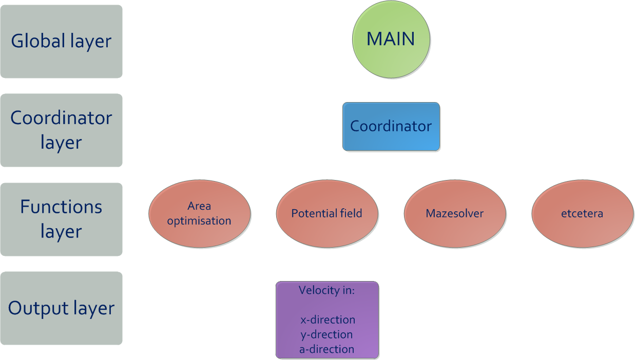
The main idea to make this challenge a success was to work in a structured way. To make sure the structure during the project would be clear a top-down approach is used. The main goal of this approach was to be easily able to determine what happens at every time when the code is ran. The highest layer is chosen to be the main file, as in the main file the whole code will be run. The next layer is the coordinator, which will determine what actions to take at any moment. It is chosen to not use multi-processing, as most of the functions' input depend on other functions' output. Therefore the performance gain would be only very little, whereas the effort would be large to implement it. The layer after that will contain all the functions. These functions will give the robot skills to complete tasks. The lowest layer is the output layer, which will generate the velocities to make Pico move.
The approach that has been used can be called rather unique: By making rectangle fits of the LRF-data the corridors can be recognized in a robust way. Using these rectangle fits setpoints can be created from intersections of rectangles. These setpoints will be stored in global coordinates in a mapping along with a direction to ensure the location of the corridor belonging to the setpoint. The odometry can be corrected using the recognition of setpoints which is based upon the rectangles. The mazesolver determines what way to go next using Tremaux’s algorithm, making sure the same road will not be driven lots of times. With a potential-field the driving can be done in a safe way, making sure there will be no collisions with the walls.
In the remaining of this wiki page the code will be explained. The coordinator that has been used and other functions will be highlighted. After that some simulations and actual performances of the robot will be shown and analyzed. At the end there will be a conclusion about what has been learned, along with some recommendations.
Coordinator
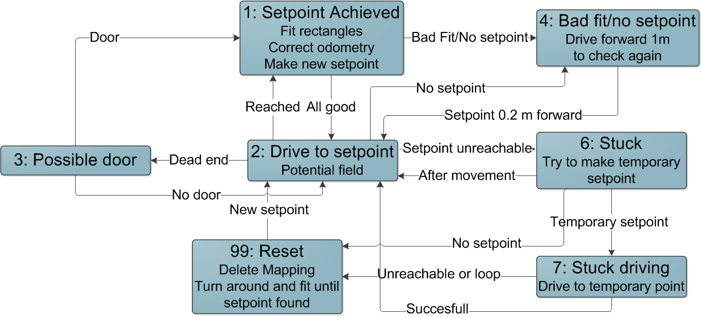
The coordinator is the function that controls in what state the robot is and what state it should go. The states are placed in a switch-case with as variable the integer "state". There are several states: Setpoint reached, Driving, Possible door, No fit or setpoint, Stuck, Stuck driving and Reset. The guards for the coordinator to get into other states are briefly shown in the figure below.
Setpoint reached
In the setpoint reached state first a new rectangle fit is made out of the laser data. The fit is analyzed to determine the possible setpoints locally. Using the local distance to the setpoint that is reached and the angle of the main rectangle the odomotry can be updated. Next, the global mapping can be updated and a new setpoint can be determined using the mazesolver. If all goes as planned the state will be updated to the driving state. If not, the state will be updated to the No fit and setpoint state.
Driving
The driving state is build up with a big if else that checks for certain situations, such as recognition of a door or the reaching of a setpoint. If some situation occurs, the state variable will be changed to make sure that the robot will be in a new state to deal with the situation properly. If there is no special situation, the robot can drive using the potential field to make sure that the robot will not collide into a wall.
Possible Door
When a door is recognized and the robot is in front of the door, the robot will get into this state. In this state a new rectangle fit will be made. After beeping and waiting for 5 seconds, a new fit will be made. The length of the rectangle in front of the robot is compared in the two situations to determine if the door has been opened. If the door has been opened, the mapping is cleared and new nodes will be made. The setpoint at the door will be set to a high value to make sure that the robot will not return through the door unless it has run through the whole maze several times. Next the state will be updated to the Setpoint reached state to make a new fit and determine new setpoints. If the door has not opened, the door was no door but a dead end and the robot will turn around to continue its search for the door.
No fit or setpoint
In this state two situations are distinguished: having an unreliable fit or having no setpoint. If the fit is reliable, but there is no setpoint, the local point that is in front of the robot with the least distance to the robot will be set as new setpoint. If the fit is unreliable, the robot will put a new setpoint 20 cm further in the corridor in which the robot is standing.
Stuck
If the robot can not reach its current setpoint it will get into this state. If the robot has no official main setpoint, as made in the first state, the robot will immediatly go to the reset state. If the setpoint cannot be reached, a temporary setpoint in the middle of the intersection will be placed, which will be driven to in the next state.
Stuck driving
In this state the robot will try to drive to the temporary setpoint. Once this setpoint is reached, the robot will go to the normal driving state to try again to drive towards the original setpoint. However, if the temporary setpoint is not reached, the robot will go to the reset state.
Reset
In this state the robot will get once things have gone wrong. All the mapping will be deleted. Next a new fit will be made and a new setpoint will be determined. If the fit is unreliable or there cannot be created a setpoint, the robot will turn 0.5 radians and try again until it has succeeded to get a reliable fit and a setpoint. Once a setpoint is determined, the state will change to the driving state.
Below is a code snippit including the first two states of the coordinator.
      switch (state)
           {
                   //1 Setpoint achieved
               case 1:
               {
                   // Make new fit
                   preprocess(scan);
                   area_optimization_algoritm(frontsight,0,false);
                   if (fit_reliable)
                   {
                       // Recognize nodes locally and convert to global coordinates
                       local_node_recognition(dv_center, side_road, relativeDirections, localcorrx, localcorry);
                       scatter_local_nodes(relativeDirections);           //Matlab scatter output for local directions for debugging
                       // Calculate odometry correction using local nodes
                       Odometry_correction(dv_center, orientationpico,localcorrx,localcorry,angle_deviation,correction_x,correction_y);
                       // Update global odometry with correction
                       updatepicoodom(odom.x,odom.y,odom.a);
                       // Save local nodes in mapping
                       globalmapping(globalDirections, relativeDirections, crossingSides, visibleDirections);
                   }
                   else
                   {
                       // If fit not reliable, go to state for small driving for new fit
                       state=4;
                       dv_center(0)=0;
                   }
                   // List all setpoints of mapping in output, also scatter of setpoints, for debugging
                   listAllGlobalDirections(globalDirections,visibleDirections);
                   // Determine which setpoint to go to next
                   Mazesolver(x,y,a);
                   if (no_setpoint)
                   {
                       // Go to state for small driving for new fit
                       state=4;
                       no_setpoint=false;
                   }
                   else //All good
                   {
                       // Go to driving state
                       state = 2;
                   }
                   break;
               }
               //2 Drive to setpoint
               case 2:
               {
                   // If dead end is recognized by mazesolver
                   if (dead_end)
                   {
                       // Go to Possible door state
                       state = 3;
                       dead_end=false;
                   }
                   // If setpoint is reached
                   else if((sqrt(square(pico_x-x)+square(pico_y-y)) < marginxy) && (fabs(fmod(((pico_a)-(a)),2*3.13)) < margina))
                   {
                       // Put velocity zero to prohibit driving while optimizing rectangles
                       io.sendBaseReference(0,0,0);
                       // Go to setpoint achieved state
                       state = 1;
                   }
                   // If no dead end nor setpoint reached, drive to setpoint
                   else
                   {
                       // Determine drive inputs
                       Potential_field(scan,x,y,a,vx,vy,va,exitflag);
                       // If the resulting force is backwards
                       if(exitflag == 5)
                       {
                           // If the setpoint is near, set the setpoint as achieved and determine new setpoint
                           if ((sqrt(square(pico_x-x)+square(pico_y-y)) < marginxy+0.3))// ||exitflag==1
                           {
                               // Determine new setpoint
                               Mazesolver(x,y,a);
                               // Determine drive inputs
                               Potential_field(scan,x,y,a,vx,vy,va,exitflag);
                           }
                           else
                           {
                               // If setpoint is not close, try to find a new setpoint
                               no_setpoint = true;
                           }
                           if (no_setpoint)
                           {
                               // Go to state for small driving for new fit
                               state=4;
                               no_setpoint=false;
                           }
                           else // All good, drive to new setpoint
                           {
                               state = 2;
                           }
                       }
                       // If stuck
                       else if(exitflag == 2 && fabs(va) < 0.1){
                           // Go to stuck state
                           state = 6;
                       }
                       else
                       {
                           // Execute driving
                           io.sendBaseReference(vx,vy,va);
                       }
                   }
                   break;
               }
               //3 Possible door
               case 3:
               {
               }
          case 6: // stuck
               {
               }
          case 7: // Stuck driving
               {
               }
           case 99: // Reset
               {
               }
          }
Environment identification
To subtract relevant information from the laser data an environment identification algorithm is used. This algorithm determines the dimensions of the corridor where pico is positioned, and it determines all the position and location of the visible sideroads. Using this information the world model can be updated, and the odometry data can be corrected.
General model
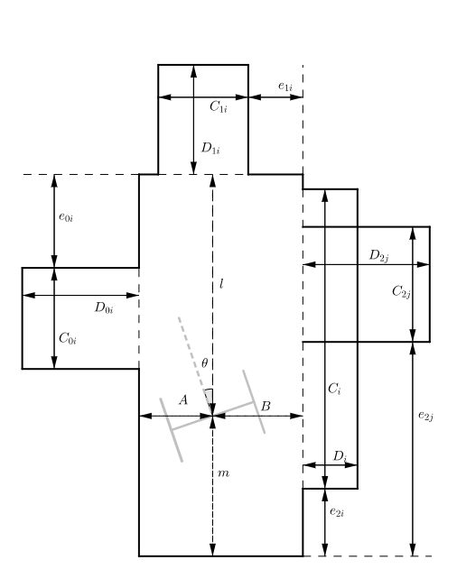
To be able to identify the environment a general model is proposed as shown in the figure to the right. The model consist of the current corridor, the corridor Pico is placed at the moment of the identification, and side roads at the west, north and east side of this current corridor.
The general model is parameterized relative to Pico. So the angle the current corridor as relative to Pico is described by [math]\displaystyle{ \theta }[/math]. The distance to the West and East walls are described with [math]\displaystyle{ A }[/math] and [math]\displaystyle{ B }[/math] respectively. To distance to the North and South are described with [math]\displaystyle{ l }[/math] and [math]\displaystyle{ m }[/math] respectively.
It is assumed that all the corridors are perpendicular to each other. Hence, each side road can be described with 3 parameters, the width ([math]\displaystyle{ C }[/math]), the length ([math]\displaystyle{ D }[/math]) and the location with respect to the current corridor ([math]\displaystyle{ e }[/math]). It is possible to detect a side road on the West, North, and East side of the current corridor, these are each identified with the numbers 0, 1 and 2 respectively. Because the LRF can not detect points behind Pico it is impossible to detect a side road on the South side of the current corridor.
The open spaces can be interpreted as a wide side road, which means a possible side road in an open space should be to overlap with the ‘side road’ connected to the open space.
Algorithm
The general algorithm consists out of the following steps
- Preprocess laser data
- Determine the dimensions of current corridor
- Determine location and dimension of side roads
- Determine reliability of the found dimensions
Preprocess laser data

First the laser data is preprocessed. The characteristics of the LRF are that in large gaps between points ‘Ghost Points’ occur. First these Ghost Points are filtered out on the basis that there are no points close to these points. Furthermore the algorithm does not need all the points from the laser data, therefore the points can be filtered such that a set of points that are really close to each other can be combined into 1 point. Using this only relevant points remain and the computation time of the algorithm increases.
Determine current corridor
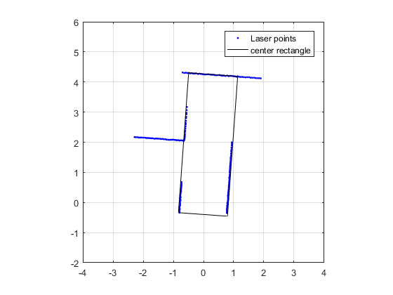
Using the relevant data the dimensions of the current corridor are determined. This is done by maximizing the area of this corridor, with the LDR data as boundary.
Optimization problem formulation
The optimization problem can be formulated as
- [math]\displaystyle{ \begin{align} &\underset{x}{\operatorname{maximize}}& & f(x)=(A+B)\cdot(l+m)=(x_1+x_2)\cdot(x_3+x_4) \\ &\operatorname{subject\;to} & & e_i(x) \leq 0, \quad i = 1,\dots,n \\ &&& x_i \leq x_{max}, \quad i = 0, \dots,4 \\ &&& x_i \geq x_{min}, \quad i = 0, \dots,4 \\ \end{align} }[/math]
where
- [math]\displaystyle{ x_0=\theta }[/math], [math]\displaystyle{ x_1=A }[/math], [math]\displaystyle{ x_2=B }[/math], [math]\displaystyle{ x_3=l }[/math], [math]\displaystyle{ x_4=m }[/math]
- the objective function [math]\displaystyle{ f(x) }[/math] is defined by the area of the rectangle,
- [math]\displaystyle{ e_i(x) }[/math]the smallest distance of point [math]\displaystyle{ i }[/math] to the sides of the rectangle, hereby the error is positive if the point is inside the rectangle
- [math]\displaystyle{ n }[/math] are the number of points.
The upper and lower bound for the design variables are chosen such that the dimensions of the rectangle stay realistic. It is assumed that Pico is positioned almost straight in the current corridor at the moment of the identification, therefore small upper and lower bounds are used for [math]\displaystyle{ \theta }[/math]
Initial conditions
From the optimization the best results are obtained when starting with feasible initial conditions. It is assumed that Pico is standing straight in the main corridor, therefore the initial condition for [math]\displaystyle{ \theta=0 }[/math]. The initial conditions for [math]\displaystyle{ A }[/math] and [math]\displaystyle{ B }[/math] are half the length of Pico, corresponding to the smallest corridor possible. The initial condition for [math]\displaystyle{ m }[/math] is also chosen small, but for the initial condition of [math]\displaystyle{ l }[/math] the LFR data in front of Pico is used. This is done because otherwise the rectangle is able to rotate in the beginning phases of the optimization, which will lead to a higher chance of a local minima.
Determine side roads
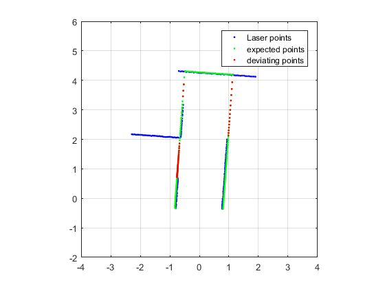
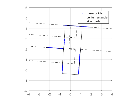
Next all the locations and dimensions of the side roads are determined. Again this is formulated as maximizing the area of a side road, with the LDR data as boundary.
Optimization problem formulation
the optimization problem can be formulated as
- [math]\displaystyle{ \begin{align} &\underset{x}{\operatorname{maximize}}& & f(x)=C\cdot D=x_1\cdot x_2 \\ &\operatorname{subject\;to} & & e_i(x) \leq 0, \quad i = 1,\dots,n \\ &&& x_i \leq x_{max}, \quad i = 1, \dots,3 \\ &&& x_i \geq x_{min}, \quad i = 1, \dots,3 \\ \end{align} }[/math]
where
- [math]\displaystyle{ x_0=e }[/math], [math]\displaystyle{ x_1=C }[/math], [math]\displaystyle{ x_2=D }[/math]
- the objective function [math]\displaystyle{ f(x) }[/math] is defined by the area of the rectangle,
- [math]\displaystyle{ e_i(x) }[/math]the smallest distance of point [math]\displaystyle{ i }[/math] to the sides of the rectangle, hereby the error is positive if the point is inside the rectangle, and
- [math]\displaystyle{ n }[/math] are the number of points.
Initial conditions
To find all side roads is a bit hard, because each side road represents a local minima in the optimization problem. It is therefore necessary to have a good guess what the location of the side road is. To obtain this good initial conditions the results from the current corridor are used. Using the dimensions of this corridor the expected LRF data without side roads can be determined. At the locations where no side road is present this expected LRF data should be close to the expected LRF data. At the locations of the side roads the expected LRF data deviates from the real LRF data, using this the initial conditions for the location and width of the side road are determined. The initial length of the side road is the minimal depth of a door to be able to detect a door, which is in fact a side road with a small length.
Determine reliability
Although the algorithm is fairly robust, in some situations it does not provide a sufficient solution. Because it is unwanted that these identifications are used in for the global mapping and odometery correction it is necessary to determine if the result is reliable.
To do this the estimated points used for the initial conditions are used again. The reliability is determined by comparing all the estimated LFR data to the real LRF data. All the estimated points which corresponds to points inside a found side road are not taken into account.
Implementation using dlib
The optimization problems in the algorithm are solved using the c++ library dlib. In this library an optimization toolbox is present. This toolbox is able to solve unconstrained optimization problems without the knowledge of the gradient of the objective function using BFGS algorithm. When an objective function is present this toolbox provides a fairly simple manner to maximize this objective function:
   find_max_using_approximate_derivatives(bfgs_search_strategy(),
            objective_delta_stop_strategy(1e-5),
            objfun_center, dv_center, 1000, 1e-5);
Note that the optimization problems in the algorithm are constrained optimization problems. To cope with this the problem formulation is transformed to an unconstrained optimization problem by applying the constraints as exterior penalty functions on the objective function.
   // Original objective function
   double f=(A+B)*(m+l);
   // Penalty for error on points
   for (int i=0; i<n; i++)
   {
       f-=n/r_point*pow(error(i),4);
   }
   // Penalty for bounds
   for (int i=0; i<5; i++)
   {
       f-=1/r_bound*pow(max(-dv_center(i)+dv_center_lb(i), 0.0),2);
       f-=1/r_bound*pow(max(dv_center(i)-dv_center_ub(i), 0.0),2);
   }
Mapping
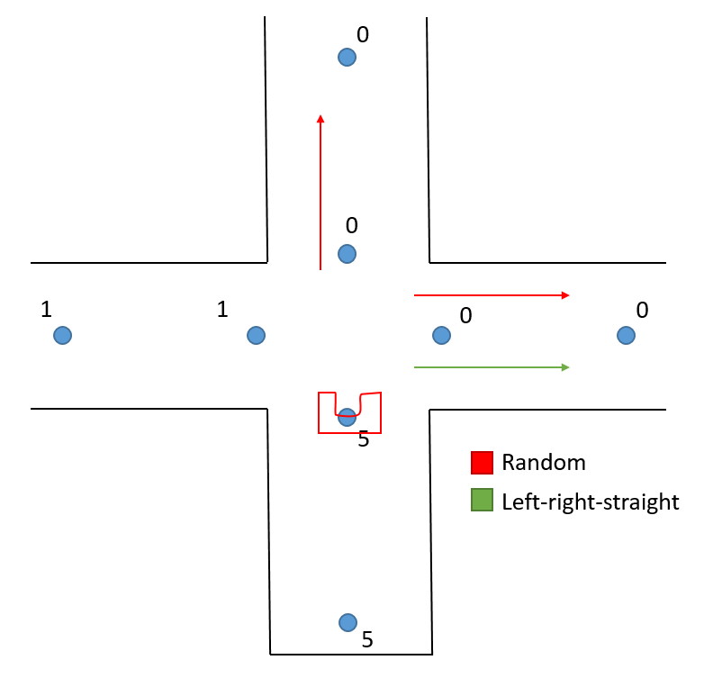
In the environment identification the current corridor and side roads are found relative to PICO. This can be translated to directions relative to PICO and positioning error relative to PICO. This is calculated in Local direction recognition. With the current location and orientation of PICO the directions relative to PICO can be rewritten to global directions from the origin. The mapping is build on the fact that the maze consists of crossings and turns. Each crossing consists of directions pointing away from the crossing. As the maze is axis aligned, all directions point either North, West, South or East. A crossing can thus be represented by multiple directions, which belong to the same intersection. A corner can be represented by two directions belonging to the same intersection, and a dead end by a single direction belonging to a intersection. In order to connect crossings, corners and dead ends the directions have to be connected. Hence the maze is represented by nodes(intersections) and edges(connected nodes) which in turn results in a undirected graph. In order to store the maze the position, orientation, intersection (number), connected direction are saved for each node together with the direction ID (which is used also for the connected direction) and the number of times that direction has been passed(which is used in the Maze solving algorithm later).
Local direction recognition
To determine local directions (the directions that PICO sees and are defined relative to PICO) the dimensions of the side roads outputted by the Environment identification are used. First it is checked whether the side roads are smaller than the maximal corridor width (1.5m). When they are smaller they will be processed as a corridor, when they're bigger as an open space. Next for all corridors the location and orientation of the direction is determined. This is the location at the crossing the current corridor(where PICO is located) in the middle of the side road that points away from the side road. In addition the furthest and closest point of each corridor is saved to distinguish separate crossings later.
A new local crossing is created and the closest and furthest point of that crossing are determined by checking when the different corridors start and end. In addition the beginning and ending widths are determined which are dependent on the presence of open spaces. All corridor directions that belong to the current local crossing are added to the list of local directions. If the crossing is in front of PICO an additional direction is added that points towards behind PICO and is located at the beginning of the crossing. If the current corridor(where PICO is located) continues after the crossing an additional direction is added that points forward and is located at the end of the crossing. A new local crossing is created and the above process repeated until all corridors are processed.
When there are no corridors left for processing the the current corridor is checked if it is a dead end. If it is a dead end then an additional direction is added with a margin from the wall, pointing away from the wall.
In the example on the right PICO is facing forward. From the results of the optimization there is a current corridor, and three side roads. Since all side roads start after the previous is finished there are 3 crossings. An additional crossing is added for the last direction belonging to a dead end. The first three directions belong to the first crossing, direction 4, 5 and 6 belong to the second crossing, direction 7(which is on the same location as direction 6), 8 and 9 belong to the third crossing and direction 10 belongs to the fourth crossing. All directions point away from the crossing.
Depending on whether the local direction recognition is called in a crossing or in a corridor it calculates the position of the end or the beginning of the first crossing. As this function is only called when a setpoint is reached this is a method to verify if PICO is on that setpoint. That location is later used to correct the odometry data.
Global mapping
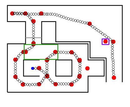

The local directions are then implemented in the global mapping and connected. To achieve this the old mapping is required, along with the local directions and the actual position and orientation of PICO.
The global mapping first saves the current global direction PICO is located if it is not connected to another node yet. For the first crossing the local direction pointing towards behind PICO is saved. If there is a local directions pointing forward and the crossing is not the last local crossing then the direction is saved as well. These are used later to connect the directions. For all directions in the current crossing all coordinates and orientations of the local directions relative to PICO are converted to be relative to the origin and then checked with all directions already in the global mapping to find matching pairs. If the local direction matches a global direction, the ID of the global direction is saved along with the crossing ID. If one direction of the local crossing is matched to a global crossing, then all local directions of that local crossing can be added to that global crossing(if they do not correspond to a global direction yet), if there is no match, then a new crossing is created where all local directions will be added. For the direction that points behind PICO it is checked wether the corresponding global direction is not connected yet. If that is the case it will be connected to the first known direction that points forward from PICO that is not matched yet(for the first direction this would be the current direction PICO is located). If there is a direction that points towards forward from PICO, and the corresponding global direction is not connected yet, this global direction is added to the list of known directions that point forward from pico that are not mached yet. This is repeated for all local crossings. The directions that are to the gobal mapping are saved and along with the earlier matched directions and together make the visible directions which could be used when PICO is lost.
At the end of the global mapping an additional function exists that cleans up the global mapping. It removes the initial direction when PICO does not have it a target direction or as last visited direction, since it is not a real crossing.
The result of the global mapping is visualized on the left and right for the maze design of 2015 and 2016. What can be seen on the left(2015) is that the mapping correctly detects directions, even for crossings that PICO has not visited yet but has seen already. In the maze on the right(2016) the green boxed intersection is an example of an intersection where (seen from the left) the right corridor starts before the left road has ended. Which is why this is considered as 1 intersection instead of 2 separate ones. Before the end of the maze there is a direction (boxed in purple) which should not be there, but is seen because of the corner in the open space. In this case it would not be a problem. If PICO ware to pick that direction, and scan the environment again it would still drive out to the final direction and drive out of the maze(this is the case in the third simulation of this years maze design below).
Odometry correction
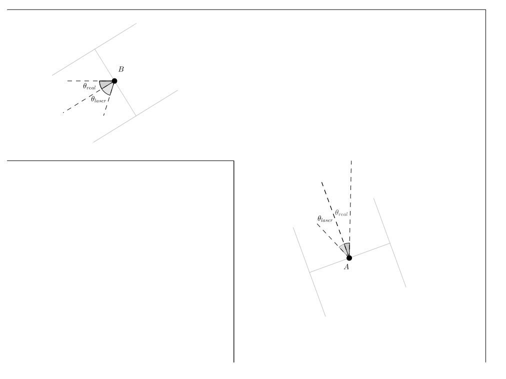
Due to slip that the Pico has in the real world, it is crucial that there is correct odometry correction. In total three corrections are introduced: the rotation, the absolute x-direction and y-direction. This is devided in two parts. Firstly, the angle correction is explained. Subsequently, the correction for the x- and y-direction is enlightened. Note that for both corrections the rectangle fits are used. Since the rectangle fit was already implemented, it would be cumbersome to not use it. Furthermore, the location of Pico has not to be precise since an accuracy of 5 cm is not an issue. Therefore, in our opinion Kalmann is a little bit of overkill.
Correction for orientation odometry
In the environment identification, rectangles are fitted which can be used to correction the angle diviation of Pico with respect to the main current corridor. As mentioned above, one of the design variables of the current corridor is the angle [math]\displaystyle{ \theta_{laser} }[/math] which is the offset off Pico. At each setpoint, a new rectangle fit is constructed. Since the direction of the setpoint is either forward, backwards, to the right, or to the left, it can be constructed what the desired odometry data should be denoted by [math]\displaystyle{ \theta_{setp} }[/math]. Furthermore, the real Pico orientation is known denoted by [math]\displaystyle{ \theta_{real} }[/math]. Subsequently, at each setpoint, when the rectangle fit is reliable, the following intuitive Equation is used to calculate the offset:
[math]\displaystyle{ theta_{deviation} = \theta_{real} - theta_{setp} - theta_{laser} }[/math]
The figure to the right is a graphical representation of this correction. Note that at each setpoint the orientation of the Pico is corrected. The final deviation of the angle is used to correct the global pico orientation odometry. Both in the simulation and during experiments this correction it was found that this correction was implemented succesfull and usefull.
Correction for x- and y-direction odometry
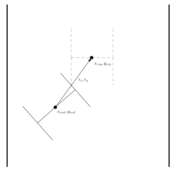
The concept for the x- and y-cirection was relatively simple. The desired setpoint was extracted from the Mazesolver given in x- and y-direction expressed with respect to the global coordinate frame noted by [math]\displaystyle{ x_{exp} }[/math] and [math]\displaystyle{ y_{exp} }[/math]. When a setpoint was reached, the function odometry correction was started. From the rectangle optimisation, it was able to locate the setpoint with respect from Pico in the local coordinate frame. These local coordinates, are transformed to the global coordinate frame using the following rotation matrix:
- [math]\displaystyle{ R = \begin{bmatrix} \cos \theta & -\sin \theta \\ \sin \theta & \cos \theta \\ \end{bmatrix} }[/math]
resulting in [math]\displaystyle{ \epsilon_x }[/math] and [math]\displaystyle{ \epsilon_y }[/math].
Since all distances are know expressed in the same global coordinate frame, the following Equations are used to determine the x- and y-deviation:
- [math]\displaystyle{ x_{cor} = x_{exp} - \epsilon_x - x_{real} }[/math]
- [math]\displaystyle{ y_{cor} = y_{exp} - \epsilon_y - y_{real} }[/math]
In the end, these corrections are applied in the global coordinate frame. However, it appeared that the applied method did not result in the expected results. The main problem was that the accuracy of the local distance from Pico to the desired setpoint was not determined correctly. Due to this reason, Pico was corrected with unreliable data. Therefore, the functioning of the mapping was bad. The second reason why this implementation of the odometry correction for x- and y-direction was not ideal, is due to the update frequency. During the simulations it appeared that the odometry correction in x- and y-direction was not bothersome, nor did it actually help. Therefore, it is suggested as a recommendation to implement another method for the odometry correction.
Mazesolver
The mazesolver makes use of the nodes which are created in the mapping. The coordinator decides when the mazesolver is ran. When the mazesolver runs it first checks if Pico is in a corridor or on an intersection. If Pico is in a corridor it looks in the list of known nodes and checks if there exists a node that is connected to the current node. If so the mazesolver will return the position of this node. Else the mazesolver will tell the coordinator that there is no connected node (the coordinator will then drive forward and try to find new nodes again). The mazesolver makes use of the Trémaux’s algorithm, when Pico reaches a node it will update the number of times Pico passed that node and it will always select the path where Pico has been the least. A dead-end is marked by updating the number of passes to 5, this way Pico will only try a dead-end once.
If Pico is on an intersection it will select the direction which Pico has passed the least. If there are multiple possible least passed directions it will select the new direction in the following order: left-right-straight. There is also a setting (which can be changed in the magic parameters) which changes the selection of the least passed direction to random.
Furthermore the mazesolver lets the coordinator know when Pico is in a dead-end and thus there is a possible door.
Potential field
One of the key elements of this project, is that Pico should be able to drive autonomously. From a higher level, the software receives a setpoint in absolute coordinates with respect to the starting position of the robot. With this information, the robot can move towards this location. However, it should also be avoided to collide into the walls. Therefore, a potential field is implemented which is a relatively easy method. The key elements are the following two forces:
- [math]\displaystyle{ F_{repp} }[/math]: Repelling force to ensure the robot will not collide with the walls
- [math]\displaystyle{ F_{attr} }[/math]: Attracting force responsible for the movement towards the setpoint
The potential field is a method from where the laser data range and angle with respect to the orientation of Pico are used. The wall forces will push Pico away from the walls, while the setpoint will attract Pico, see the Figure.
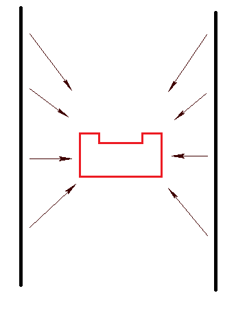
For every laser range and angle, the following Equation is executed to calculate the force vector of that data point:
[math]\displaystyle{ F_{repp,i} = \frac{1}{1375r_i^3 - 232.5r_i^2 + 12.19r_i} }[/math]
![Schematic representation of total force on Pico together with angle [math]\displaystyle{ \phi }[/math]](/images/Total_force.png)
where the three constants of the polynomial expression are used to optimize the repelling force vectors. Afterwards, the contribution in the x- and y-direction can be computed with help of the angle for each laser data. The attracting force is computed by the following Equation:
[math]\displaystyle{ F_{attr} = e_x^2 + e_y^2 }[/math]
in where [math]\displaystyle{ e_x }[/math] and [math]\displaystyle{ e_y }[/math] are the relative error between Pico and the setpoint in meters. Afterwards, this force is normalised to ensure that [math]\displaystyle{ F_{attr} }[/math] will not go to zero when Pico is almost at the desired setpoint. Note that [math]\displaystyle{ F_{attr} }[/math] is with respect to the base coordinate frame. Since [math]\displaystyle{ F_{rep} }[/math] is in the relative coordinate frame, [math]\displaystyle{ F_{attr} }[/math] is rewritten to relative coordinates with a rotation matrix as used earlier in odometry correction.
The parameters above are scaled in such a way that the following desired behaviour is exacted:
- When Pico is located close to a wall, [math]\displaystyle{ F_{rep} \gt \gt F_{attr} }[/math]
- When Pico is not located at a close distance to a wall, [math]\displaystyle{ F_{rep} \lt \lt F_{attr} }[/math]
Subsequently, the total force [math]\displaystyle{ F_{tot} }[/math] is calculated. From here, an angle [math]\displaystyle{ \phi }[/math] is obtained which can be used to calculate the desired velocities in the x- and y-direction, see the Figure.
Afterwards, the velocity in x- and y-direction of the Pico is calculated by
- [math]\displaystyle{ v_{x} = \text{cos}(\phi)v_{max} }[/math]
and
- [math]\displaystyle{ v_{y} = \text{sin}(\phi)v_{max} }[/math].
Additionally, when the total force angle is behind Pico, Pico will first start turning around before driving to the setpoint, to prevent Pico from driving backwards. This is dangerous due to the fact there is no laser data available at the back of Pico. For the rotational velocity, the error between the setpoint orientation and Pico's current rotation is used.
Solved problems
Once a week a experimental session was planned to test the written code. This usually introduced problems because of situations that ware not thought of, or because of uncertainties in the real world. A number of these problems are described below, as well as the solutions that ware implemented to solve these problems
- Robot does not reset the odometry data when a new piece of code is executed. A initialization function was created that saves the initial position and rotation(the initial odometry data). Each new odometry data is then compared to the initial odometry data to obtain the corrected odometry.
- Number of laser data points is not equal to 1000 as suggested in the simulator. Therefore, the values of minimum angle and maximum angle differ. Additionally, when there is a laser data point from where no object is visible, the laser data becomes infinity resulting in problems in the Potential field. These problems were found during the experiments and fixed in that week.
- The local direction detection only checked the first intersection it saw in front of PICO. For the odometry correction a direction is needed that could also lie behind PICO. Therefore the local direction recognition is rewritten to detect all crossings it can see, such that all information that PICO has would be processed in the mapping and directions behind PICO could also be used for correction.
- When PICO is at the start of a small corridor, and sees a side road on either side behind itself, a local direction would be detected for this side road. However when the laser data ends before the side road ends, the width of the side road would not be correct, and also the direction would be faulty, resulting in a non existent direction. During area recognition it can be seen that these side roads start as soon as the laser data starts. For each of these side roads it is passed along to the local direction recognition whether this is the case or not. The side roads that have this are not processed in the mapping, but could be processed for correction, since the end of the side road(closest to pico) is detected correctly.
- Because the odometry correction did not work as well as hoped some errors occurred in the mapping. One of these errors is that local directions are not matched to a global direction, while they should be while others are. For example when the local direction(A) should be recognized as an already existing global direction but isn't. However when the connected local direction(B) is recognized as a global direction the first local direction (A) will not be connected while it should. This is an indication that local direction (A) is a faulty direction. Therefore direction A is removed from the mapping, as other directions that should be connected but aren't.
Simulations and attempts
Corridor challenge simulation
As can be seen in the video below the robot is able to do the corridor challenge. The robot follows two setpoints that are placed on the intersection edges. The setpoints are made using the rectangle fit and driving is done using the potential field.
Corridor challenge attempt
During the real corridor challenge the robot behaved as expected. Our code used the same speed or cornering, as for straight paths. Since there ware some issues with PICO doing corners fast, the speed was lowered. This meant however, since the corridor was very long, that the time was not very fast: the robot could have driven faster on the straight. This is something that might be implemented for the maze challenge. We did get a nice compliment about the smooth cornering though! A link to the video of the corridor challenge is shown below.
https://www.youtube.com/watch?v=upn1WE3GwSs
Maze simulations
To prepare for the maze challenge multiple mazes ware created by hand, but the best test is that of the maze design of 2015. Which are are shown below. In the both simulations the maze solver chooses the direction on the crossing based on the number of passes of the directions. It picks the direction with the least passes. If the number of passes are equal the simulation on the left has a preference for left, then right, then straight, the simulation on the right picks one of the least passed direction at random. In both cases the maze is solved. In the situation on the right one can see the Tremaux algorithm picking visiting all the directions before picking the direction that leads to the door. No direction is passed more than 3 times. Both simulations are sped up with 150%.
Maze challenge attempts
On June 8th 2016, the final Maze challange was held at the RoboCup soccer field. In total, 7 groups implemented their code on PICO to see which group was able to finish the maze. Each group had two attempts at solving the maze. The maze is depicted below and as one can see consists of multiple dead-ends, one loop, a rather tricky placed door, and an open-space. The starting position was the U-shaped corridor in the bottom of the figure. The open-space was located behind the door. At the end of the open-space, the exit was located. Below, the two attempts are discussed together with the results and a video of the challanges.
Attempt 1
Below, a YouTube-link to the first attempt of the Maze challange at the RoboCup soccer field can be found. For the first attempt, the Mazesolver introduced a preference with respect to which direction PICO should go at an intersection. When PICO approaches an intersection, the first preference is to the left, the second preference to the right and else PICO should go straight.
https://www.youtube.com/watch?v=8nTIp-3s3bo
It is observed that the initialisation is executed correctly, since PICO correctly fits the rechtangles and goes to the left at the initial intersection. Afterwards, PICO recognizes the second intersection and decides to go to the left again. Unfortunately, due to the unlucky placement of the door PICO did not recognize the intersection including the door. Therefore, PICO drives forward and goes to the left afterwards. Due to the preference to the left, PICO drives back to it's starting position. However, the Tremaux algorithm ensures that PICO does not visit places where it already have been. Therefore, it goes to the right at the intersection, hence it can be concluded that the mapping was executed correctly. Unfortunately, PICO detects a dead-end which results in a turn-around. This is due to the fact that the rectangle fit does not 'see' the corridor to the right, and therefore marks the corridor as a dead-end. Subsequently, PICO drives to the starting position. From then on, PICO starts panicking and undesired actions are happening resulting in a collission with the wall. The problem of the wrongly detected dead-end could be fixed by implementing a certain trust region in the local node recognition. That is that only in a certain region around PICO, local nodes should be recognized. However, this re-adjustment will have consequences for the rest of the code and therefore was not implemented easily during the Maze challange.
Attempt 2
Below, the YouTube-link to the second attempt of the Maze challange can be found. Since the first attempt was not succesfull, another method of the Mazesolver was implemented. This time, PICO randomly chooses a direction to go when PICO is at an intersection. Maybe PICO was now able to atleast find the door and open it.
https://www.youtube.com/watch?v=J7_U3Ru8vq4
From the video, it is observed that again the initialisation phase was succesfull. Note that this time PICO randomly chooses to go to the right at the second intersection. Unforunately, PICO again approaches the door from the side for which is it difficult to recognize the door. From that on, PICO start panicking again and does undesired actions. However, PICO was able to reset hisself resulting in a clean slate resulting in correctly taking turns. Sadly, PICO again recognizes a dead-end due to the fact that one side-road is not fitted correctly. Therefore, PICO turns around. After multiple can find the door and is able to open the door, although a little bit of luck was needed. Unfortunately, PICO did not enter the open-space and was therefore not able to finish te Maze.
Simulation
After the maze challenge the maze design is used in the simulator to run the algorithm. For the simulations the maze solver was run on the setting that picks the least used direction. If there are multiple least used directions, then it picks one of these at random. Because of this the maze should be solved with different paths which can be seen below. For this the odometry correction is disabled, since in the simulator the odometry data corresponds with the actual position and rotation. Below each animation there is commentary. All three simulations are sped up with 150%.
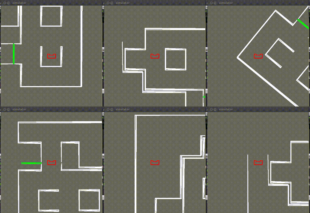
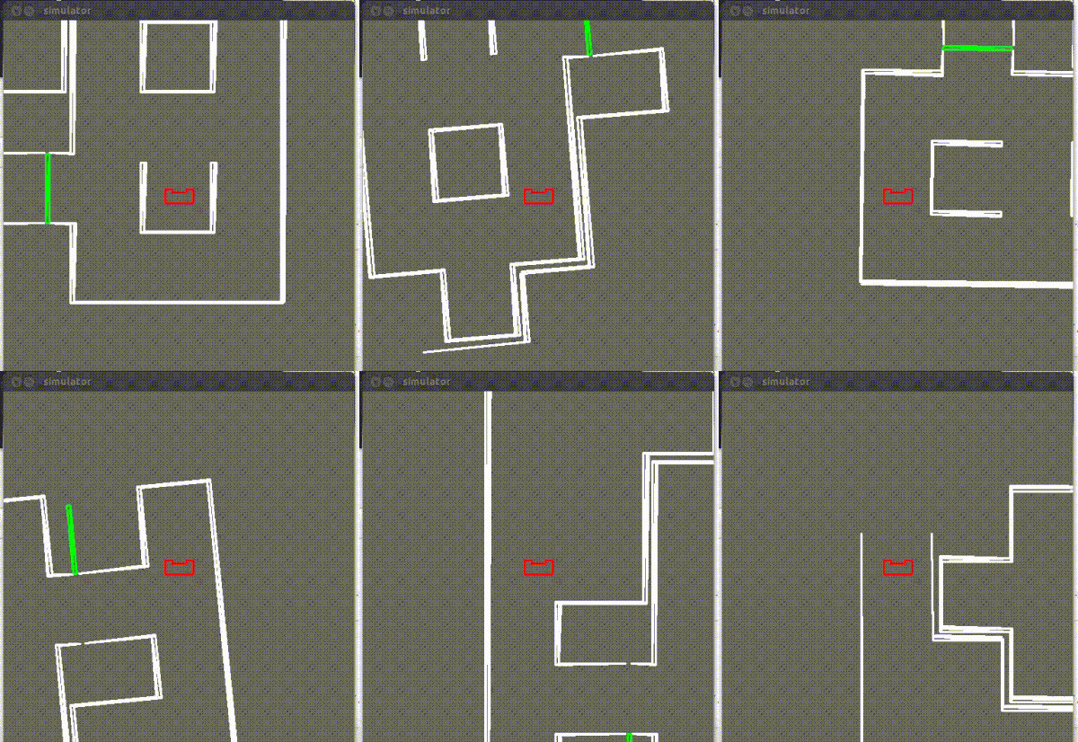

Overall Conclusion
Conclusion
During this group-project we learned a lot regarding coding in C++, but also using a compact code architecture. It turned out that our approach was different and unique compared to all other groups. The rectangle fit idea was worked out and used as one of the main functions used for other code components such as local node recognition and the mapping. Although the rectangle idea seemed wonderful on the first hand because the solution would be easily scaleable to different situation, there are some drawbacks. One of the biggest drawback is that the local node extraction is complex to implement. Furthermore, the odometry correction should have been implemented in a different manner since the current odometry correction was not reliable enough due to the low update rate. It appears that there is always room for improvement. Furthermore, programming in C++ was a new experience for most of us. The EMC environment provided on Ubuntu gave us the tools to develop our program skills, and gave us hand on experience of embedding the code on an actual robot which was really great. To conclude, the biggest lessons learned during this project are:
- The effectiveness of a coordinator
- When the main file is explicitly separated in multiple files, the structure from the composition pattern is easier to understand
- Simulation does not guarantee correct performance during experiments
- Start with a correct model-formulation before writing C++ code
- Start easy
- Make sure that the magic parameters are defined to ensure that the code is easily scaleable
- How to ensure robustness and take undesired behaviour into account
- Communication is important! It is of great importance to have regular sessions with the group and communicate about the processes of each group-member.
Recommendation
As mentioned earlier, there is always room for improvement. When we had some more time to improve, the following aspects could be improved:
- Odometry correction: as mentioned earlier, the current implementation is not reliable enough to ensure proper correction. Therefore, another method should be implemented, preferably using the rectangle fits.
- Local node recognition: the current node recognition works fine, however there is still room for improvement. During the Maze challange it appeared that the trust region of the local node recognition should be lowered to ensure that corridors are not characterised as dead-ends.
- Visualisation: it is always nice to have some fancy visual aids which can be used for debugging. For example, the vectors of the potential field could be represented, as well as the global mapping including the position of PICO.
Files
Initial Design: File:Initial design.pdf
Presentation of task-skill-motion system architecture: File:System architecture Presentation Group 7.pdf
Presentation of final design: File:Final design.pdf
