Mobile Robot Control 2024 Ultron:Solution 4: Difference between revisions
| Line 64: | Line 64: | ||
==== 2.1 Correct the particles with LiDAR ==== | ==== 2.1 Correct the particles with LiDAR ==== | ||
'''1. What does each of the component of the measurement model represent, and why is each necessary.''' | '''1. What does each of the component of the measurement model represent, and why is each necessary.''' | ||
The measurement model consists of hit, short, maximum range, and random models. The hit model calculates the probability of the measured value being close to the predicted value, using a Gaussian distribution to handle sensor noise. The short model handles cases where the measured value is less than the predicted value, accounting for unexpected close-range obstacles. The maximum range model deals with measurements reaching the sensor's maximum range, often indicating no obstacle detection. The random model addresses random noise in the measurements, covering irregular measurement errors. | |||
'''2. With each particle having N >> 1 rays, and each likelihood being ∈ [0, 1], where could you see an issue given our current implementation of the likelihood computation.''' | '''2. With each particle having N >> 1 rays, and each likelihood being ∈ [0, 1], where could you see an issue given our current implementation of the likelihood computation.''' | ||
Revision as of 11:42, 7 June 2024
0. Assignment introduction
0.1 Explore the code framework
1.How is the code is structured?
- The code for this assignment is organized into multiple classes, with each object or component having its own class and functions that allow for modifying its specific aspects.
2.What is the difference between the ParticleFilter and ParticleFilterBase classes, and how are they related to each other?
- Differences:
ParticleFilterBaseprovides the basic functionalities and interfaces of the particle filter, including particle initialization, propagation, weight computation, and setting resampling strategies.ParticleFilterinherits fromParticleFilterBaseand implements specific update and resampling strategies. It extends the base class by providing concrete implementations for theupdateandconfigureResamplermethods.
- Relationship:
ParticleFilteris a subclass ofParticleFilterBase, inheriting all its attributes and methods while overriding or extending some of them to provide additional functionalities.
3.How are the ParticleFilter and Particle class related to eachother?
- The
ParticleFilterclass manages and utilizes a set ofParticleinstances for filtering operations. It inherits fromParticleFilterBaseand implements particle propagation, weight calculation, and resampling by invoking methods onParticleobjects.ParticleFilterinitializes particles, propagates their states based on odometry data, calculates weights from sensor measurements, and resamples according to the configured strategy. TheParticleclass encapsulates the attributes and behaviors of individual particles, such as state initialization, propagation, and likelihood computation.ParticleFiltercoordinates the filtering process, whileParticlerepresents and updates individual states.
4.Both the ParticleFilterBase and Particle classes implement a propagation method. What is the difference between the methods?
- The
propagateSamplesmethod in theParticleFilterBaseclass propagates all particles, typically called in the main loop of the particle filter to update the state of all particles. In contrast, thepropagateSamplemethod in theParticleclass propagates a single particle, usually invoked by thepropagateSamplesmethod inParticleFilterBase, to update the state of a specific particle.
1. Assignments for the first week
1.1 Initialize the Particle Filter
1. What are the advantages/disadvantages of using the first constructor, what are the advantages/disadvantages of the second one?
- First Constructor (Uniform Distribution)
- Advantages:
- The wide coverage ensures that all possible states are taken into account and is therefore suitable for completely unknown initial states.
- Disadvantages:
- The efficiency is relatively low because in known environments it may be low due to the fact that many particles may be placed in irrelevant regions.
- Convergence is slower and may take longer to converge to the true state, especially in large environments.
- Advantages:
- Second Constructor (Gaussian Distribution)
- Advantages:
- The search is more focused because the particles are concentrated near the known mean value, thus speeding up convergence.
- More efficient in scenarios with some prior knowledge of the initial state, placing particles where they are more likely to find the true state quickly.
- Disadvantages:
- Relies on having a reasonable estimate of the initial state. Incorrect initial mean can lead to incorrect convergence.
- The coverage is limited because the true state may be missed if it is not within the initial Gaussian distribution.
- Advantages:
2. In which cases would we use either of them?
- When choosing between constructors, it depends on the application's context and the knowledge of the initial state. Use the first constructor (uniform distribution) when the initial state is completely unknown, such as at system startup or in a complex, unknown environment, as it ensures broad coverage. Use the second constructor (Gaussian distribution) when there is prior knowledge of the initial state, such as in tracking known targets or when previous state estimates are available, as it allows for focused and efficient search, leading to faster convergence.
1.2 Calculate the pose estimate
1. Interpret the resulting filter average. What does it resemble? Is the estimated robot pose correct? Why?
- The filtered average is essentially a weighted average of the particles, providing a single estimate of the state of the system. This estimate is calculated based on the position and weight of each particle. The principle is that particles with higher weights contribute more to the average than particles with lower weights.
- The current filter average is the filter average of all particles under the same weights. The current filter average could not correctly estimate the robot's pose without additionally updating the weights based on additional information.
2. Imagine a case in which the filter average is inadequate for determining the robot position.
1.3 Propagate the particles with odometry
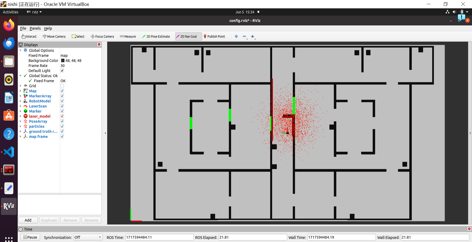
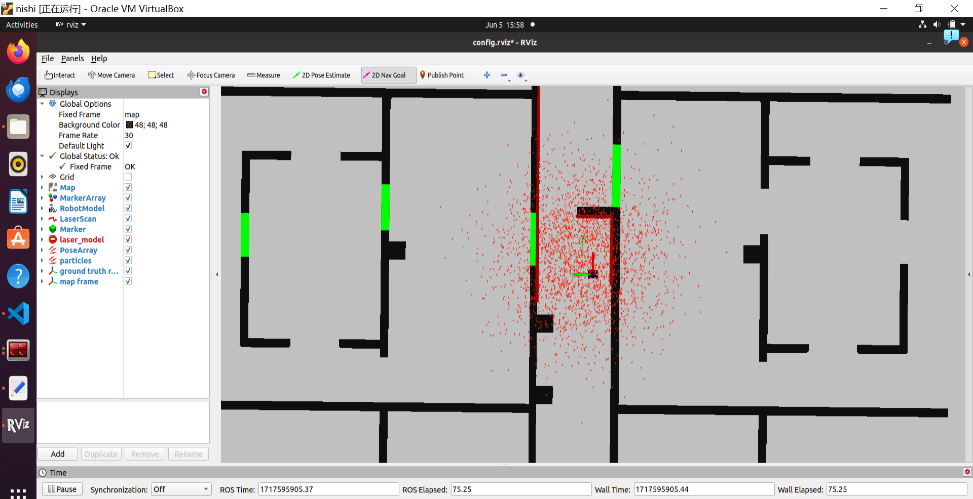
The screenrecodring of rviz can be seen in Propagate the particles with odometry
1. Why do we need to inject noise into the propagation when the received odometry infromation already has an unkown noise component?
2. What happens when we stop here, and do not incorporate a correction step?
2. Assignment for the second week
2.1 Correct the particles with LiDAR
1. What does each of the component of the measurement model represent, and why is each necessary.
The measurement model consists of hit, short, maximum range, and random models. The hit model calculates the probability of the measured value being close to the predicted value, using a Gaussian distribution to handle sensor noise. The short model handles cases where the measured value is less than the predicted value, accounting for unexpected close-range obstacles. The maximum range model deals with measurements reaching the sensor's maximum range, often indicating no obstacle detection. The random model addresses random noise in the measurements, covering irregular measurement errors.
2. With each particle having N >> 1 rays, and each likelihood being ∈ [0, 1], where could you see an issue given our current implementation of the likelihood computation.
2.2 Re-sample the particles
1. What are the benefits and disadvantages of both the multinomial resampling and the stratified resampling?
2. With each particle having N >> 1 rays, and each likelihood being ∈ [0, 1], where could you see an issue given our current implementation of the likelihood computation?
2.3 Test on the physical setup
1. How you tuned the parameters.
2. How accurate your localization is, and whether this will be sufficient for the final challenge.
3. How your algorithm responds to unmodeled obstacles.
4. Whether your algorithm is sufficiently fast and accurate for the final challenge.

