Mobile Robot Control 2024 Wall-E

Group members:

Caption

Name	student ID
Coen Smeets	1615947
Sven Balvers	1889044
Joris Janissen	1588087
Rens Leijtens	1859382
Tim de Wild	1606565
Niels Berkers	1552929

Exercise 1

Instructions

1. Create a folder called exercise1 in the mrc folder. Inside the exercise1 folder, create an src folder. Within the src folder, create a new file called dont_crash.cpp.
2. Add a CMakeLists.txt file to the exercise1 folder and set it up to compile the executable dont_crash.
3. Q1: Think of a method to make the robot drive forward but stop before it hits something. Document your designed method on the wiki.
4. Write code to implement your designed method. Test your code in the simulator. Once you are happy with the result, make sure to keep these files as we will need them later.
5. Make a screen capture of your experiment in simulation and upload it to your wiki page.

Implementations:

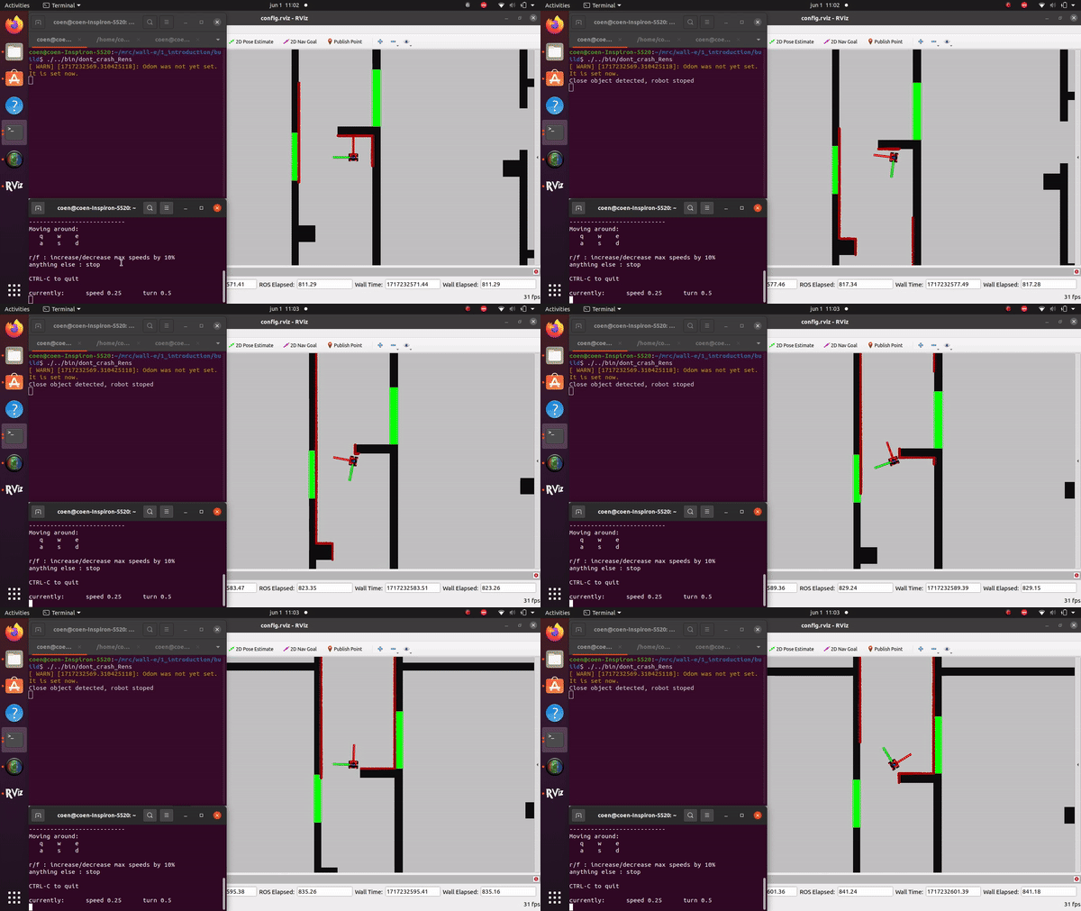
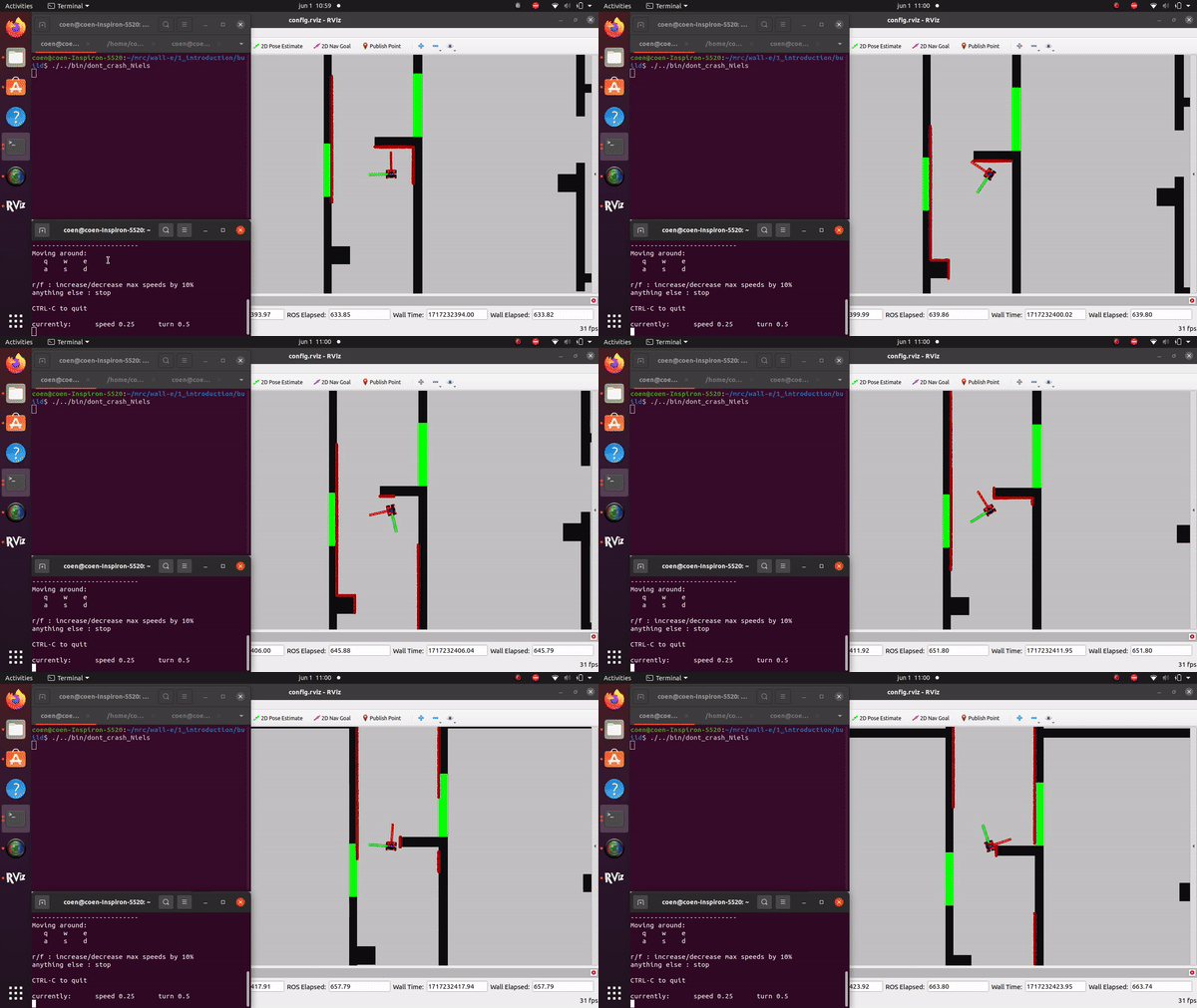
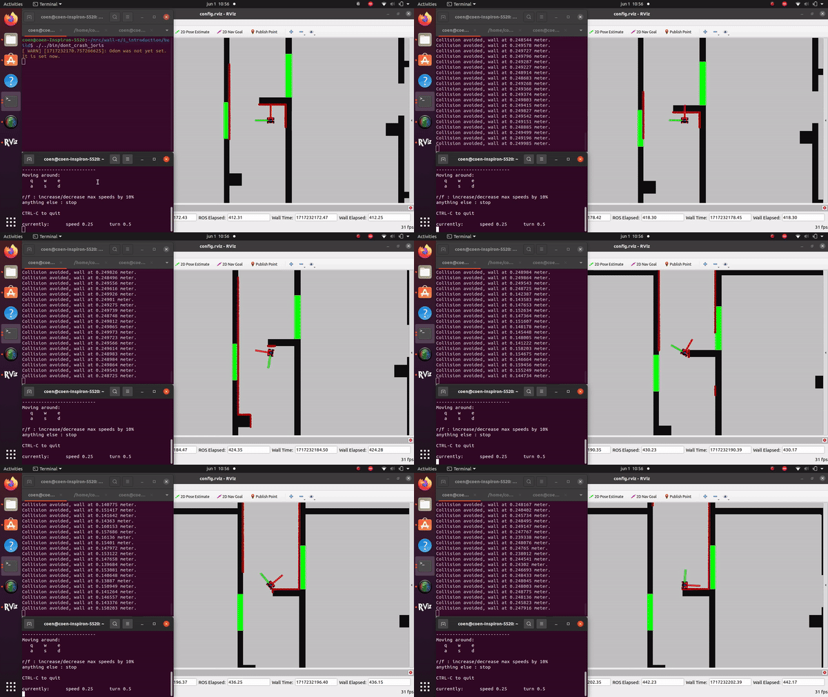
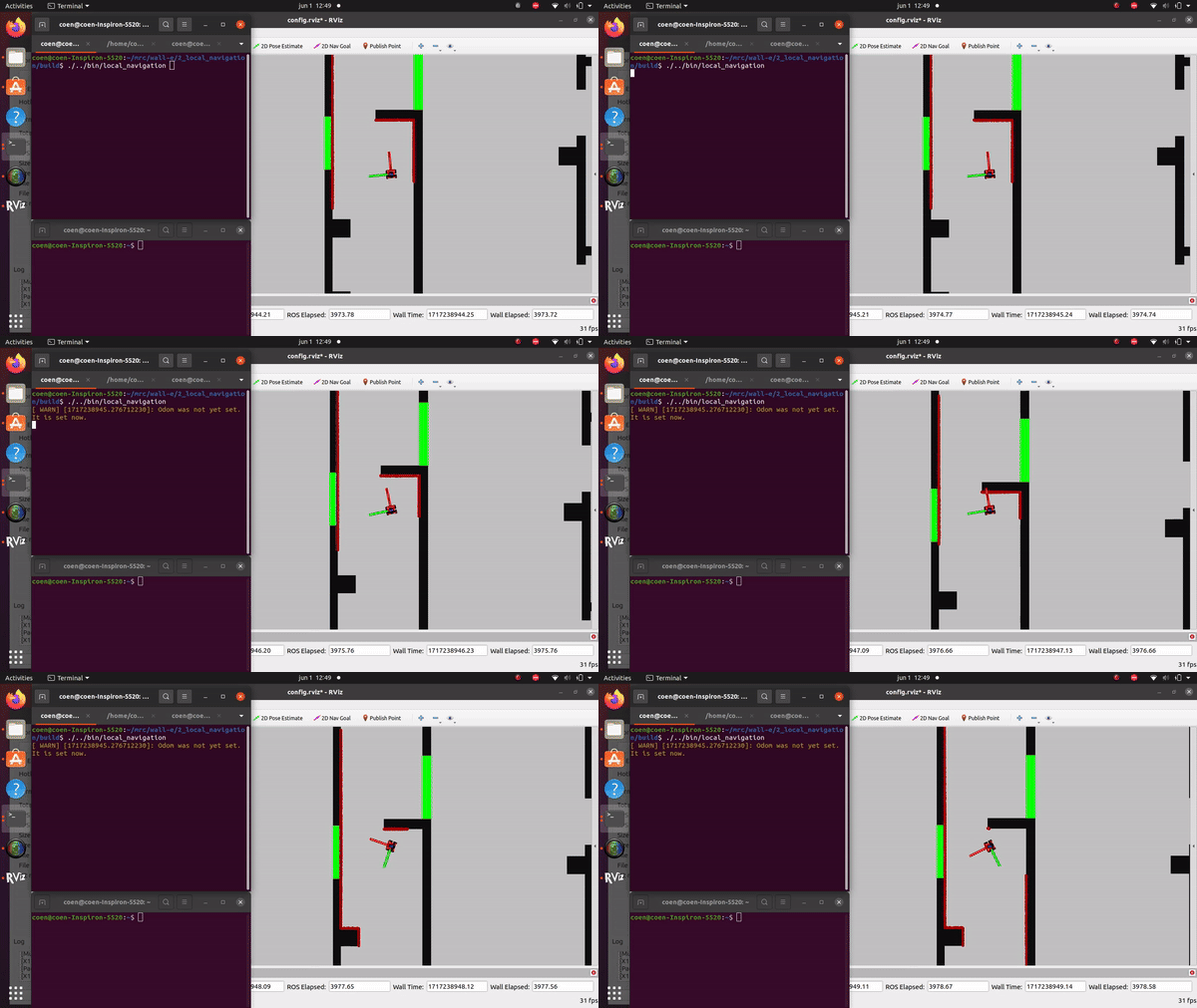
The videos for the don't crash simulations have been made with the use of the Teleop command. The inputs differ per video, however, the same logic for where to go has been used. Firstly, the drive forward and do not hit a will is tested. Then a corner is tested while driving closely next to a wall. As the teleop overwrites the 0 velocity input of the don't crash, it may be difficult to see that the robot is stopping. Take into account that if the robot is jolty, it is being stopped by the don't crash code.

Coen Smeets:

Dont Crash Coen: This don't crash experiment shows how Coen's version only looks at rays that are in front of the robot. Thus, it is allowed to drive close next to a wall.

The provided C++ code is designed to prevent a robot from colliding with obstacles by using laser scan data and odometry data. Here's a step-by-step explanation of how it works:

1. Initialization: The code starts by initializing the emc::IO object for input/output operations and the emc::Rate object to control the loop rate. It also initializes some variables for later use.
2. Main Loop: The main part of the code is a loop that runs as long as the io.ok() function returns true. This function typically checks if the program should continue running, for example, if the user has requested to stop the program.
3. Reading Data: In each iteration of the loop, the code reads new laser scan data and odometry data. If there's new data available, it processes this data.
4. Processing Odometry Data: If there's new odometry data, the code calculates the linear velocity vx of the robot by dividing the change in position by the change in time. It also updates the timestamp of the last odometry data.
5. Collision Detection: If there's new laser scan data, the code calls the collision_detection function, which checks if a collision is likely based on the laser scan data. If a collision is likely and the robot is moving forward (vx > 0.001), the code sends a command to the robot to stop moving. It also prints a message saying "Possible collision avoided!".
6. Sleep: At the end of each iteration, the code sleeps for the remaining time to maintain the desired loop rate.

This code ensures that the robot stops moving when a collision is likely, thus preventing crashes.

Collision detection function

The collision_detection function is a crucial part of the collision avoidance code. It uses laser scan data to determine if a collision is likely. Here's a step-by-step explanation of how it works:

The collision_detection function is a crucial part of the collision avoidance code. It uses laser scan data to determine if a collision is likely. Here's a step-by-step explanation of how it works:

1. Function Parameters: The function takes four parameters: scan, angle_scan, distance_threshold, and verbose. scan is the laser scan data, angle_scan is the range of angles to consider for the collision detection (default is 1.7), distance_threshold is the distance threshold for the collision detection (default is 0.18), and verbose is a boolean that controls whether the minimum value found in the scan data is printed (default is false).
2. Zero Index Calculation: The function starts by calculating the index of the laser scan that corresponds to an angle of 0 degrees. This is done by subtracting the minimum angle from 0 and dividing by the angle increment.
3. Minimum Distance Calculation: The function then initializes a variable min_value to a large number. It loops over the laser scan data in the range of angles specified by angle_scan, and updates min_value to the minimum distance it finds.
4. Verbose Output: If the verbose parameter is true, the function prints the minimum value found in the scan data.
5. Collision Detection: Finally, the function checks if min_value is less than distance_threshold and within the valid range of distances (scan.range_min to scan.range_max). If it is, the function returns true, indicating that a collision is likely. Otherwise, it returns false.

This function is used in the main loop of the code to check if a collision is likely based on the current laser scan data. If a collision is likely, the code sends a command to the robot to stop moving, thus preventing a crash.

Potential improvements:

While the current collision detection system is effective, it is sensitive to outliers in the sensor data. This sensitivity can be problematic in real-world scenarios where sensor noise and random large outliers are common. Safety is about preparing for the worst-case scenario, and dealing with unreliable sensor data is a part of that. Here are a couple of potential improvements that could be made to the system:

1. Rolling Average: One way to mitigate the impact of outliers is to use a rolling average of the sensor data instead of the raw data. This would smooth out the data and reduce the impact of any single outlier. However, this approach would also introduce a delay in the system's response to changes in the sensor data, which could be problematic in fast-moving scenarios.
2. Simplifying Walls to Linear Lines: Given that the assignment specifies straight walls, another approach could be to simplify the walls to linear lines in the data processing. This would make the collision detection less sensitive to outliers in the sensor data. However, this approach assumes that the walls are perfectly straight and does not account for any irregularities or obstacles along the walls.

   "- All walls in the restaurant will be approximately straight. No weird curving walls." [1](https://cstwiki.wtb.tue.nl/wiki/Mobile_Robot_Control_2024)

   This process involves several steps that may not be immediately intuitive. Here's a breakdown:
   1. Data Cleaning: Remove outliers from the data. These are individual data points where the sensor readings are clearly incorrect for a given time instance.
   2. Data Segmentation: Divide the data into groups based on the angle of the sensor readings. A group split should occur where there is a significant jump in the distance reading. This helps differentiate between unconnected walls.
   3. Corner Detection: Apply the Split-and-Merge algorithm to each wall. This helps identify corners within walls, which may not be detected by simply looking for large jumps in distance.

Keep in mind that the complexity of the scene can significantly impact the computation time of this algorithm. However, given the scenes shown on the wiki, the additional computation time required to generate clean lines should be minimal. This is because the number of walls is relatively small, and the algorithm can be optimized in several ways. For instance, instead of processing each data point, you could select a subset of evenly spaced points. On average, these selected points should accurately represent the average location of the wall.

Based on my experience, prioritizing safety enhancements in the system is crucial. Establishing a strong safety foundation from the outset is key. By implementing robust safety measures early in the development process, we can effectively mitigate potential risks and issues down the line.

Dont Crash Rens: This Dont Crash version takes all rays into account thus it cannot drive close to a wall.

Rens Leijtens

General structure

• including libraries
• main starts
  • initialization of objects and variables
  • while loop that is active while io.ok() is true
    • the laser and odometry data is checked and processed
    • the movement is enabled or disabled if necessary

The included libraries are the following:

• iostream for print to terminal
• emc/rate for fixed loop time
• emc/io for connecting with the simulated robot

Movement

The movement is controlled using a simple boolean called "move" which will move the robot if true and stop the robot if false.

Sensor data processing

Check if data is new

check if a measurement point is closer than 0.2 meters then the robot will stop moving.

Improvements

this method also measures the side notes which will not be optimal if the robot needs to pass through a small hallway.

Dont Crash Niels: This Dont Crash version takes all rays into account thus it cannot drive close to a wall.

Niels Berkers:

The code uses the standard library header <iostream>, which is used when printing outputs to the terminal. Furthermore, the <emc/io.h> package provides the structures and functions to read data from the LiDar sensor and other hardware information needed for robot movement. Finally the package <emc/rate.h> is used to set the appropriate frequency for a while loop.

Implementation:

After the packages are included the main function is called, which starts by creating an IO object of the class IO and setting the frequency to 10 Hz. Afterwards, a while loop starts running that only breaks if the IO tools are not ok. Inside the while loop the reference velocity is set so that the robot drives forward with a velocity of 0.1. Afterwards, if new laser data is obtained, it loops over all indexes of the scan data and checks if the a range is within 0.3 meters. If that is the case, the reference velocity is set to 0 for all directions and thus the robot stops driving.

Improvements:

The code can be improved by only looking at a window that is in front of the robot. When this would be implemented, it would also be possible to drive parallel and close to a wall. This would also decrease the amount of indexes that need to be checked. The code can also be improved by sending out a signal when the robot is too close to a wall, which could be handy in a future and possibly bigger algorithm.

Joris Janissen:

Dont Crash Joris: This don't crash experiment shows how Joris's version looks only ahead of the robot and thus the robot can drive closely next to a wall. However, it does not detect corners perfectly and thus there is an incident.

Packages Used

• emc/io.h: This package provides functionalities for interfacing with hardware, including reading laser and odometry data, and sending commands to control the robot's movement.
• emc/rate.h: This package enables control over the loop frequency, ensuring the code executes at a fixed rate.
• iostream: This package facilitates input/output operations, allowing for the printing of messages to the console.
• cmath: This package provides mathematical functions used in the implementation.

Implementation

• Initialization: The main() function initializes the IO object, which initializes the input/output layer to interface with hardware, and creates a Rate object to control the loop frequency.
• Data Processing: Within the main loop, the code reads new laser and odometry data from the robot. It then calculates the range of laser scan indices corresponding to a specified angle in front of the robot.
• Obstacle Detection: The code iterates over the laser scan data within the specified range. For each laser reading, it checks if the range value falls within the valid range and if it detects an obstacle within a certain stop distance threshold.
• Action: If an obstacle is detected within the stop distance threshold, the code sends a stop command to the robot and prints a message indicating the detected obstacle and its distance. Otherwise, if no obstacle is detected, the code sends a command to move the robot forward.
• Loop Control: The loop sleeps for a specified duration to maintain the desired loop frequency using the r.sleep() function.

Improvements

1. Data segmentation: The data points can be grouped to reduce computation time.
2. Collision message: The collision message now spams the terminal, it can be improved to plot only once.
3. Rolling average: The rolling average can be taken from the data points to filter out outliers or noise.

Conclusion

This documentation provides insights into the implementation of obstacle avoidance using laser scans in a robotic system. By leveraging the EMC library and appropriate data processing techniques, the robot can effectively detect obstacles in its path and navigate safely to avoid collisions, there are however some improvements.

Dont Crash Sven: This Dont Crash version takes all rays into account thus it cannot drive close to a wall.

Sven Balvers:

implementation:

Header Files: The code includes some header files (emc/io.h and emc/rate.h) which contain declarations for classes and functions used in the program, as well as the standard input-output stream header (iostream).

Main Function: The main() function serves as the entry point of the program.

Object Initialization: Inside main(), several objects of classes emc::IO, emc::LaserData, emc::OdometryData, and emc::Rate are declared. These objects are part of a framework for controlling a robot.

Loop: The program enters a while loop that runs as long as io.ok() returns true. This indicates that the I/O operations are functioning correctly, and thus is connected.

Control Commands: Within the loop, it seems to send a reference command to the robot's base at a fixed rate of 5 Hz using io.sendBaseReference(0.1, 0, 0). This command tells the robot to move forward at a certain velocity.

Data Reading: It reads laser data and odometry data from sensors attached to the robot using io.readLaserData(scan) and io.readOdometryData(odom).

Obstacle Detection: If new laser data or odometry data is available, it checks the laser scan data for any obstacles within a certain range (less than 0.3 units). If an obstacle is detected, it sends a stop command to the robot's base using io.sendBaseReference(0, 0, 0), setting the value of the speed to 0.

Rate Control: The loop sleeps for a fixed duration (r.sleep()) to maintain the specified loop rate.

Improvements:

To prevent the noise of the measurement data there are multiple approaches, we can take a moving average of the samples this will cause a delay of the data. We can also take point near one another to merge as one point and taking the average. Than there isn't a delay present.

Another improvement that can be made is to limit the vision of the robot to a certain angle and not the full range from -pi to +pi. This will ensure the robot is able to pass through a narrow hall, which is important for the final code.

Dont Crash Tim: This Dont Crash version takes all rays into account thus it cannot drive close to a wall.

Tim de Wild

Improvements:

Dont Crash real life test. It shows that it detects a wall and instead of driving into it, it will turn left. Due to the noise of the Lidar it is rather jolty when turning as it sees objects in front of it sometimes and thus stops rotating.

Exercise 1 (practical)

You now know how to work with the robot. For your first session, we suggest you start by experimenting with the robot. Document the answers to these questions on your wiki.

Go to your folder on the robot and pull your software.

On the robot-laptop open rviz. Observe the laser data. How much noise is there on the laser? What objects can be seen by the laser? Which objects cannot? How do your own legs look like to the robot.

The noise of the signal from the robot's Lidar is difficult to quantify, as noticed during testing of "dont_crash" file. When the robot drives straight towards an object, it stops abruptly, but when it approaches a wall at a sharp angle, it stutters slightly. This happens because only a limited number of data points are obtained in such cases, making the noise on the sensor apparent. The robot can only see object at the hight of the Lidar. The Lidar has a distribution of measuring points spreading a certain angle. Due to this, the Lidar can have problems detecting thin objects such as chair legs. Objects it can observe are flat surfaces. The robot's scanning capability doesn't cover a full 360 degrees around itself but instead sees a 180-degree angle centered at the front.

Take your example of don't crash and test it on the robot. Does it work like in simulation? Why? Why not? (choose the most promising version of don't crash that you have.)

The Don't crash code runs almost the same as the simulations. One important remark can be made about not running into people. The Lidar sees the legs of a person. However, feet extend drastically further out than the legs. Thus, the robot runs over feet as it sees the legs and think that it still has space left.

The most promising version of the code is Coen's version. This is due to the fact that it does not look at the full range but only the relevant rays in front of the robot. It can thus, in comparison to other implementations, drive close to walls that are to the side of it. This this especially relevant in narrow hallways.

If necessary make changes to your code and test again. What changes did you have to make? Why? Was this something you could have found in simulation?

We modified the code so that the robot doesn't stop when it reaches a wall but instead turns left until it has enough space to resume driving. What's noticeable is that the robot starts and stops repeatedly because it can drive a short distance and then stops again. To prevent this, the robot should turn slightly longer to maintain continuous movement. We could see this in the simulation however we only created this code to try when we were there.

From the real life test, it become apparant that some of the data might need to receive some smoothing. During turning some random measurements appear in front of the robot (To the side but just within the range that Coen's version tests). It thus become Jolty in turning. It can be solved in multiple ways. Firstly, don't crash can only prevent lateral velocity and not rotational. This will fix the issue that the robot rotates and still stops. The data can also be cleaned first with the use of a rolling average, however, this is not wanted at high velocities and low Lidar frequencies as measurements can differ more.

Local Navigation

Artificial Potential Field

Background

Artificial Potential Field is to treat the robot's configuration as a point in a potential field that combines attraction to the goal, and repulsion from obstacles. The resulting trajectory is output as the path. This approach has advantages in that the trajectory is produced with little computation. However, they can become trapped in local minima of the potential field and fail to find a path, or can find a non-optimal path. The artificial potential fields can be treated as continuum equations similar to electrostatic potential fields (treating the robot like a point charge), or motion through the field can be discretized using a set of linguistic rules. A navigation function or a probabilistic navigation function are sorts of artificial potential functions which have the quality of not having minimum points except the target point.

The Algorithm

The APF algoritm makes use of the position of the robot [math]\displaystyle{ q }[/math] and the position of the goal point [math]\displaystyle{ q_g }[/math] to compute the error between the two as [math]\displaystyle{ e(q) = q_g - q }[/math]. This error is used to compute the attractive force as seen below, where [math]\displaystyle{ k_a\gt 0 }[/math]. The magnitude of the attractive force is normalised and multiplied with a factor [math]\displaystyle{ k_a }[/math].

[math]\displaystyle{ f_a(q) = -\nabla U_a(q) = k_a \frac{e(q)}{\left\Vert e(q) \right\Vert} }[/math]

The error [math]\displaystyle{ e(q) }[/math] is also used to compute the repulsive force field, the formula can be seen below where [math]\displaystyle{ k_r\gt 0 }[/math], [math]\displaystyle{ \eta_i(q) }[/math] is the range value of a single LiDAR data point, and [math]\displaystyle{ \eta_0 }[/math] is the threshold for a scanned obstacle where the repulsive force field kicks in. The repulsive force is the force pushing the robot away from nearby objects scanned by the LiDAR data to prevent collisions.

[math]\displaystyle{ f_{r,i}(q) = -\nabla U_r(q) = \begin{cases} \frac{k_r}{\eta_i^2(q)}(\frac{q}{\eta_0} - \frac{1}{\eta_i(q)})\nabla\eta_i(q) & \text{if $\eta_i(q) \leq \eta_0$} \\ 0 & \text{if $\eta_i(q) \gt \eta_0$} \end{cases} }[/math]

The total Artificial Potential Field is computed as [math]\displaystyle{ f(q) = f_a(q) + \sum_{i=1}^p f_{r,i}(q) }[/math], where [math]\displaystyle{ p }[/math] is the total amount of LiDAR data points used. Right now they are not all used, since 1000 is unnecessary much. Each 10th LiDAR data point is used, resulting in 100 range values. The amount of range values can be changed and [math]\displaystyle{ k_r }[/math] will scale accordingly.

The shape of the formula dependent on [math]\displaystyle{ \theta_f }[/math] that multiplies with [math]\displaystyle{ f(q) }[/math].

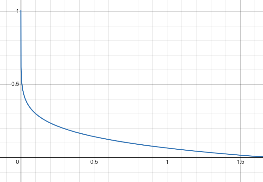
After the gradient field [math]\displaystyle{ f(q) }[/math] is calculated, it has to be translated to velocity inputs for the mobile robot. These velocity inputs come down to linear velocity and angular velocity: [math]\displaystyle{ \dot{q}=\begin{bmatrix} v\\ \theta \end{bmatrix} }[/math]. The calculation for the velocity is given below, where [math]\displaystyle{ \theta_f }[/math] is the angle the force field directs the robot to move in relative to the robot itself. The angular velocity input is determined by [math]\displaystyle{ \theta_f }[/math] and the forward velocity is determined by the magnitude of the force field on the location of the robot times a formula dependent on [math]\displaystyle{ \theta_f }[/math]. The shape of this formula can be seen in the figure on the right. When the force field pushes the robot straight ahead, the full magnitude of the force is utilized. However, when the force field directs the robot to turn, the forward velocity input is minimal, with a minimum of 0.08 m/s.

[math]\displaystyle{ v = \begin{bmatrix} \text{max}\left(1-\left(\frac{|\theta_f|}{\pi}\right)^{(\frac{1}{8})},0.08\right) \frac{1}{0.92} - 0.08\\ \theta_f \end{bmatrix} }[/math]

Simulation and testing videos

It can be seen that hallways in the direction of the goal point are not a problem. It is a problem whe the robot has to drive perpendicular to the goal point to make progress.

Goal point at the end of the hallway. It can be seen that APF enters a local minima as soon as the left wall is in the picture. With the local minima detector it is fixed.

It can be seen that it again enters a local Minimum which is then subsequently solved. (Parameters are not tuned perfectly to show the workings of the local minimum solver.

It even finds a safe way through the small gap at the third block.

This environment ended up being too challanging without intermediate goal points to traverse safely. A global planner with smaller path segments will solve this issue.

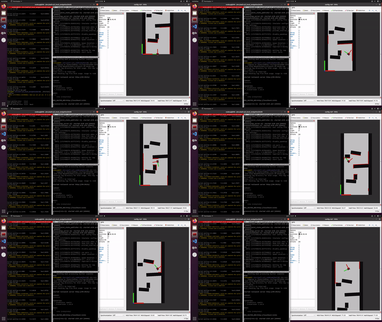
The robot in the simulation video below follows 3 goal points, these are not placed optimally as a robust global path planner should do. This is done on purpose to make sure the robot has to maneuver around obstacles to follow the path. It can be seen that the robot follows the path quite smoothly. If the goal points are positioned extremely bad, for example behind a wall, the algorithm will come in a local minimum and after some time ask for a new goal point that is reachable.

(Simulation video made, only needs to be uploaded)

Advantages

One of the main advantages is the simplicity of the algorithm. It can be implemented with straightforward mathematical functions. Another advantage is the robot will always avoid obstacles and drive in a smooth path (if it doesn't encounter a local minimum.

Disadvantages

The main disadvantage is that the robot can become stuck in a local minimum or in al local minimum loop and will not reach its end goal. The effectiveness of the method heavily depends on the tuning of parameters like the strength of the attractive and repulsive potentials. Improper tuning can lead to poor performance. The method relies on local information and does not inherently consider the global environment. This can result in sub optimal paths or failure to find a path in complex environments. But this is where the global path finding comes in to action.

Real life test of the global and local path planning algorithm in the map_compare map, the localisation is based on odometry data.

Solutions

First, the robot should never get stuck in a local minimum if the global path finding is sufficiently robust. However, if this does occur, two solutions have been implemented. Firstly, if the robot remains in a local minimum for 2.5 seconds and its position does not change significantly, the driving force will gradually be increased to help the robot escape. The second solution implemented is the detection of a situation where the robot remains in a local minimum for 30 seconds. The robot will then indicate that it wants an alternative route to reach its destination. This is done because the environment is dynamic and cannot be fully predicted.

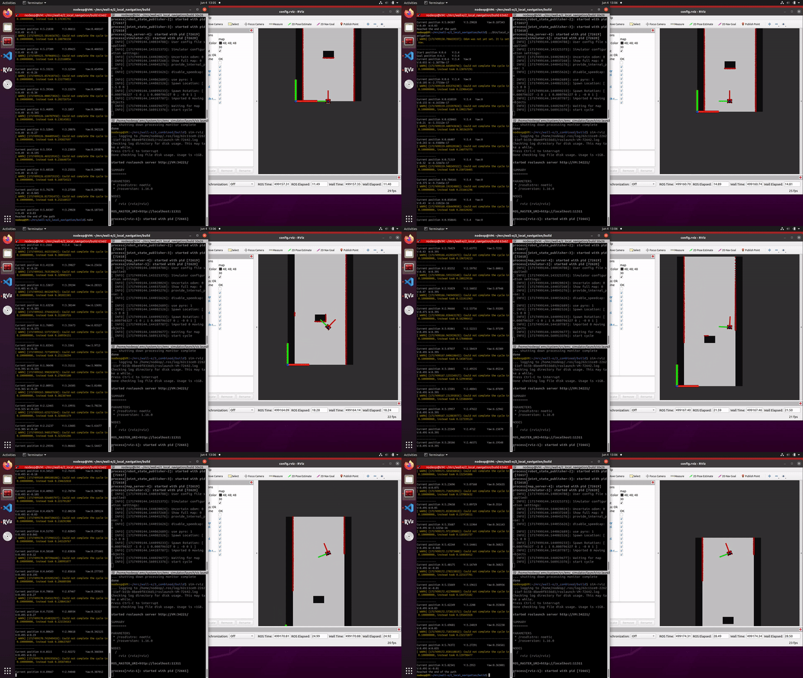
To implement the integration of local planning with global planning, the global planner provides a list of way points for the local planner to follow. As the robot approaches a way point on the list, it switches to the next point on the list until the robot reaches its final destination. A real life example of how the global and local path planner work together can be seen in the video on the right. The problem here is that the dimensions of the "hero" robot are used and not the dimensions of the "bobo" robot. This results in the robot having some difficulties driving trough the straight hallway at the end. Also can't the robot localize itself, this is now done based on the starting position and the odometry data.

Dynamic Window Approach

Background

The Dynamic Window Approach (DWA) serves as a local navigation algorithm tailored for mobile robots. It functions by analyzing both the present condition of the robot and the array of conceivable future states within a dynamically adaptable "window" of acceptable velocities and angular velocities. Each potential future state undergoes evaluation based on factors like its proximity to the goal, its clearance from obstacles, and its feasibility within the dynamic constraints of the robot.

The Algorithm

The computeDynamicWindow function calculates the permissible range of linear and angular velocities for the robot based on its current state and dynamic constraints. It determines the minimum and maximum linear velocities by considering the robot's current velocity, the maximum acceleration, and the time step:

[math]\displaystyle{ v_{min} = max(v_{min}, v - a_{max} \triangle t) }[/math]

[math]\displaystyle{ v_{max} = min(v_{max}, v + a_{max} \triangle t) }[/math]

Similarly, it computes the minimum and maximum angular velocities using the current rotational velocity, the maximum allowable yaw rate, and the time step:

[math]\displaystyle{ \omega_{min} = max(-\omega_{max}, \omega - \alpha_{max} \triangle t) }[/math]

[math]\displaystyle{ \omega_{max} = min(-\omega_{max}, \omega + \alpha_{max} \triangle t) }[/math]

The number of possible linear and angular velocities is then determined based on the specified resolution:

[math]\displaystyle{ n_{velocities} = \frac{v_{max} - v_{min}}{\small{\text{Velocity resolution}}} }[/math]

[math]\displaystyle{ n_{yawrates} = \frac{\omega_{max} - \omega_{min}}{\small{\text{Yawrate resolution}}} }[/math]

Memory is allocated for arrays to store these possible velocities, and each velocity value is assigned iteratively within the specified range. Finally, the function returns the dynamic window containing the calculated permissible velocities.

The calculateVelocityCost function determines the cost associated with the current linear velocity of the robot. It calculates the following cost by subtracting the current forward velocity from the maximum permissible velocity specified in the parameters:

[math]\displaystyle{ \text{VelocityCost} = \text{maxVelocity} - \text{forwardVelocity} }[/math]

This operation provides insight into how far the robot's velocity deviates from the maximum allowable value. The

The calculateHeadingCost function evaluates the robot's orientation towards a goal, determining the cost of its current heading. This cost measures how well the robot is aligned with the goal. The function calculates the angle between the robot's current position and the goal point, then compares this angle to the robot's current heading. The absolute value of this difference is taken as the heading cost, which reflects how directly the robot is oriented toward its target

The calculateClearanceCost function calculates the cost associated with the clearance of the robot from obstacles in its environment. It iterates over a simulated time horizon, updating the robot's pose based on its velocity. Within each time step, it iterates over the laser scan data transformed into a point cloud. For each point in the point cloud, it computes the distance between the robot's pose and the obstacle point in the world frame. It further transforms this distance into the robot's local frame to account for its orientation. The function updates the minimum clearance distance if a closer obstacle is detected. After iterating over all laser scan points within the time horizon, it returns the reciprocal of the minimum clearance distance as the clearance cost. If the robot is within a minimum threshold distance from an obstacle, it returns the maximum possible clearance cost.

The optimalInputVelocity function determines the optimal velocity input for the robot based on the given laser scan data, odometry data, current pose, current velocity, and goal position. It first transforms the laser scan data into a point cloud in the world frame. Then, it computes the dynamic window based on the transformed point cloud, current pose, and velocity. Within nested loops iterating over possible velocities and yaw rates within the dynamic window, it computes the cost associated with each velocity and yaw rate combination. The cost is calculated as a weighted sum of the forward velocity cost, the heading cost towards the goal, and the obstacle clearance cost, each multiplied by their respective parameters:

[math]\displaystyle{ G(v, \omega) = k_h \cdot h(v, \omega) + k_d \cdot d(v, \omega) + k_s \cdot s(v, \omega) }[/math]

Where:

• [math]\displaystyle{ h(v, \omega) }[/math]represents the target heading cost towards the goal.
• [math]\displaystyle{ h_k }[/math] represents the weight of the heading cost.
• [math]\displaystyle{ d(v, \omega) }[/math] represents the distance to the closest obstacle on the trajectory.
• [math]\displaystyle{ h_d }[/math] represents the weight of the clearance cost.
• [math]\displaystyle{ s(v, \omega) }[/math] represents the forward velocity.
• [math]\displaystyle{ h_s }[/math] represents the weight of the velocity cost.

The function then selects the velocity input with the minimum total cost. Additionally, it checks if the goal has been reached within a threshold distance and returns a tuple containing the optimal velocity, a boolean indicating whether the goal has been reached, and a boolean indicating if a new global path needs to be planned. Simplified pseudo code for calculating the optimal input velocity using DWA would look like:

 Function optimalInputVelocity(scanData, odometryData, pose, vel, goal):
   dw ← computeDynamicWindow(pose, vel)
   total_cost ← ∞

   For i from 0 to dw.nPossibleVelocities - 1 Do:
     For j from 0 to dw.nPossibleYawrates - 1 Do:
       forwardVelocity ← dw.possibleVelocities[i]
       rotationalVelocity ← dw.possibleYawrates[j]

       iPose ← calculateNewPose(pose, forwardVelocity, rotationalVelocity, dt)
       cost ← costForwardVelocity * calculateVelocityCost(iVelocity) +
                costTargetHeading * calculateHeadingCost(iPose, goalPoint) +
                costObstacleClearance * calculateClearanceCost(iPose, iVelocity, scanData)

       If cost < total_cost Then:
         total_cost ← cost
         optimalVelocity ← iVelocity

   goalReached ← distanceToGoal < goalDistanceMargin
   Return (optimalVelocity, goalReached, false)

DWA parameters

Parameter	Value	Unit
minVelocity	0.0	m/s
maxVelocity	0.25	m/s
maxAcceleration	0.2	m/s^2
maxYawrate	0.4	rad/s
maxdYawrate	0.4	rad/s
velocityResolution	0.005	-
yawrateResolution	0.005	-
dt	0.2	s
maxTime	3.0	s
costWeightHeading	0.05	-
costWeightClearance	2.0	-
costWeightVelocity	0.3	-

Simulation and testing videos

Global Navigation

Probabilistic Road Map

It must be noted that this section has been heavily influenced by Coen Smeets's BEP report. Ideas and abstracts have been taken from this report as it was written by a groupmember.

A visualisation of how Uniform, random and Halton placement of points in 2D space compare. The benefits of Halton, uniform yet random, can be identified

Probabilistic Road Maps, henceforth noted as RPM, are a method of creating a network in which a dedicated algorithm can find the shortest route. In order to be a good network for the purpose of navigating a mobile robot, the network has to be a correct representation of the enviroment where safety is of importance; Edges between nodes are safe. There are several methods to create a network, however, Tsardoulias et al. (2016) compared several techniques to optimise path planning and concluded that space sampling methods are most effective in two-dimensional Occupancy grid map, OGM. The data for the environment has been pre-parsed to an occupancy grid map by the course. Space sampling shows great success rate, small execution times and short paths without excessive turns.

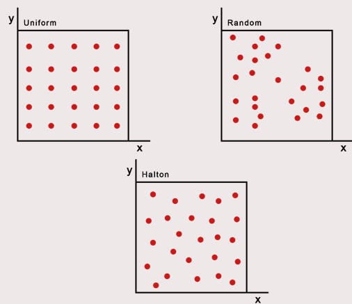
For space sampling, the Halton sequence technique presented in Tsardoulias et al. (2016) has been adapted to create a network, G. The network is a simplified representation of the movable space in the OGM. The Halton sequence combines the advantages of random sampling and uniform sampling. In random sampling, every cell can be sampled independently of its location, ensuring an unbiased representation. On the other hand, uniform sampling ensures that the sampled points are evenly distributed. Therefore, the Halton sequence offers the benefits of both approaches simultaneously. The network will consist of nodes, the sampled points in the OGM, and links between nodes, possible paths. The Halton sequence has low discrepancy and thus appears random while being deterministic. It samples the space quasi-randomly but with an even distribution. The space is sampled in 2D by using a sequence of bases 2 and 3. The higher the base the more computationally demanding the calculations are, thus, base three is chosen in the evaluation between evenly spreading the nodes and computational power. The sequences are subsequently scaled to the space the OGM takes up by using the number of rows and columns for the x and y coordinates, respectively and with the use of the resolution of the map.

The created two-dimensional Halton sequence contains the possible locations of nodes within the OGM. However, each node is additionally checked to determine whether it is located within a cell that is considered free. This check is necessary as the area spanned by all free cells can still contain occupied cells. Nodes should also not be placed in free cells close to occupied cells where collisions between the robot and the obstruction still occur. Free cells close to occupied cells are found by 'inflating' the occupied cells. This process operates by iterating over each pixel in the map, and if the pixel is identified as part of an obstacle, it sets the surrounding pixels within a specified radius to also be part of the obstacle.

When all nodes are placed, edges are created between each node with specific rules to ensure safety and an efficient network. Firstly, each edge should not surpass a distance threshold. This is mostly to optimise the second rule's calculations where it states that each edge should not pass through an occupied cell. This safety rule is checked with the use of Bresenham's line algorithm. Bresenham's line algorithm is an efficient method used in computer graphics for drawing straight lines on a grid by minimizing the use of floating-point arithmetic and rounding errors. Edges are only placed when they are safe and not unnecessarily long. An additional minimum threshold for the distance can be added but by the use of the Halton sequence, as explained above, a certain uniformness in distribution of the quasi-random points can be assumed.

Combining these principles of placing nodes and edges, create a coherent network in an environment expressed in an occupancy grid map. This network is subsequently used in the A* path planning algorithm.

Psuedo Code

 Function HaltonSequence(size, base):
   sequence ← []
   For i ← 1 to size Do
     f ← 1
     r ← 0
     while i > 0 Do
       f ← f / base
       r ← r + f * (i mod base)
       i ← floor(i / base)
     sequence.append(r)
   Return sequence

 Function BresenhamLine(x0, y0, x1, y1):
   points ← []
   dx ← abs(x1 - x0)
   dy ← abs(y1 - y0)
   sx ← if x0 < x1 then 1 else -1
   sy ← if y0 < y1 then 1 else -1
   err ← dx - dy
   while True Do
     points.append((x0, y0))
     If x0 == x1 and y0 == y1 Then
       Break
     e2 ← 2 * err
     If e2 > -dy Then
       err ← err - dy
       x0 ← x0 + sx
     If e2 < dx Then
       err ← err + dx
       y0 ← y0 + sy
   Return points

A* path planning

Background

The A* (A-star) algorithm is a popular and widely used path finding and graph traversal algorithm. It is especially well-known for its use in applications such as AI in games, robotics, and GPS navigation systems. The A* algorithm combines the strengths of Dijkstra's algorithm and Greedy Best-First-Search to efficiently find the shortest path between nodes in a graph. Staring form a specific node, it aims to find a path to the given goal node having the smallest cost. It does this by maintaining a tree of paths originating at the start node and extending those paths one edge at a time until the goal node is reached. At each iteration the algorithm needs to determine which part to extend. It does this by taking in to account the cost to come and the heuristic cost to go to the end node. The heuristic cost is can be different for different implementations of the algorithm, here however it is the absolute distance between the node that is being checked and the final node. It is important that the heuristic cost is never over estimated. The algorithm described so far gives us only the length of the shortest path. To find the actual sequence of steps, the algorithm can be easily revised so that each node on the path keeps track of its predecessor. After this algorithm is run, the ending node will point to its predecessor, and so on, until some node's predecessor is the start node.

Questions & Answers

More efficient note placement

A more efficient way of placing the nodes is to place nodes only in the corners where the robot would, or can change direction, this makes the graph easier to navigate due to the fewer points present. See figure below.

https://dsdwiki.wtb.tue.nl/images/Beter_node_placement.png

Halton node placement already improves, as previously noted, both the randomness and the uniformess over a grid or a random approach. Thus, there is already a more efficient note placement in place.

Is RPM for a maze efficient

It is not a good idea to use RPM for a maze since RPM is not well suited for narrow hallways. Points have to be randomly placed and will not be placed in the middle of the hallway. Thus, limiting the capacility. However, a grid approach has a similar problem where the grid should line up with the narrow hallway, otherwise the entire hallway will not be seen.

APF is combined with the global path planner. It creates a path and then effectively follows the path safely.

What would happen if the map updates?

If the map is updated, the robot will first attempt to follow the pre-determined path with the local planner. If it encounters a local minimum and cannot proceed, the robot will request a new global route and continue from its current position. This can be due to a limitation of the local navigation or because the path is not possible anymore due to the dynamic environment. If the second reason is the case, the map will be updated and a new path will be planned.

Test the combination of your local and global planner for a longer period of time on the real robot. What do you see that happens in terms of the calculated position of the robot? What is a way to solve this?

Due to the pose data being solely based on odometry data, the ground-truth will deviate from the calculated pose. Thus, the real robot is not following the correct path in the correct place anymore. This is solved by the use of active localisation. More can be read on this later.

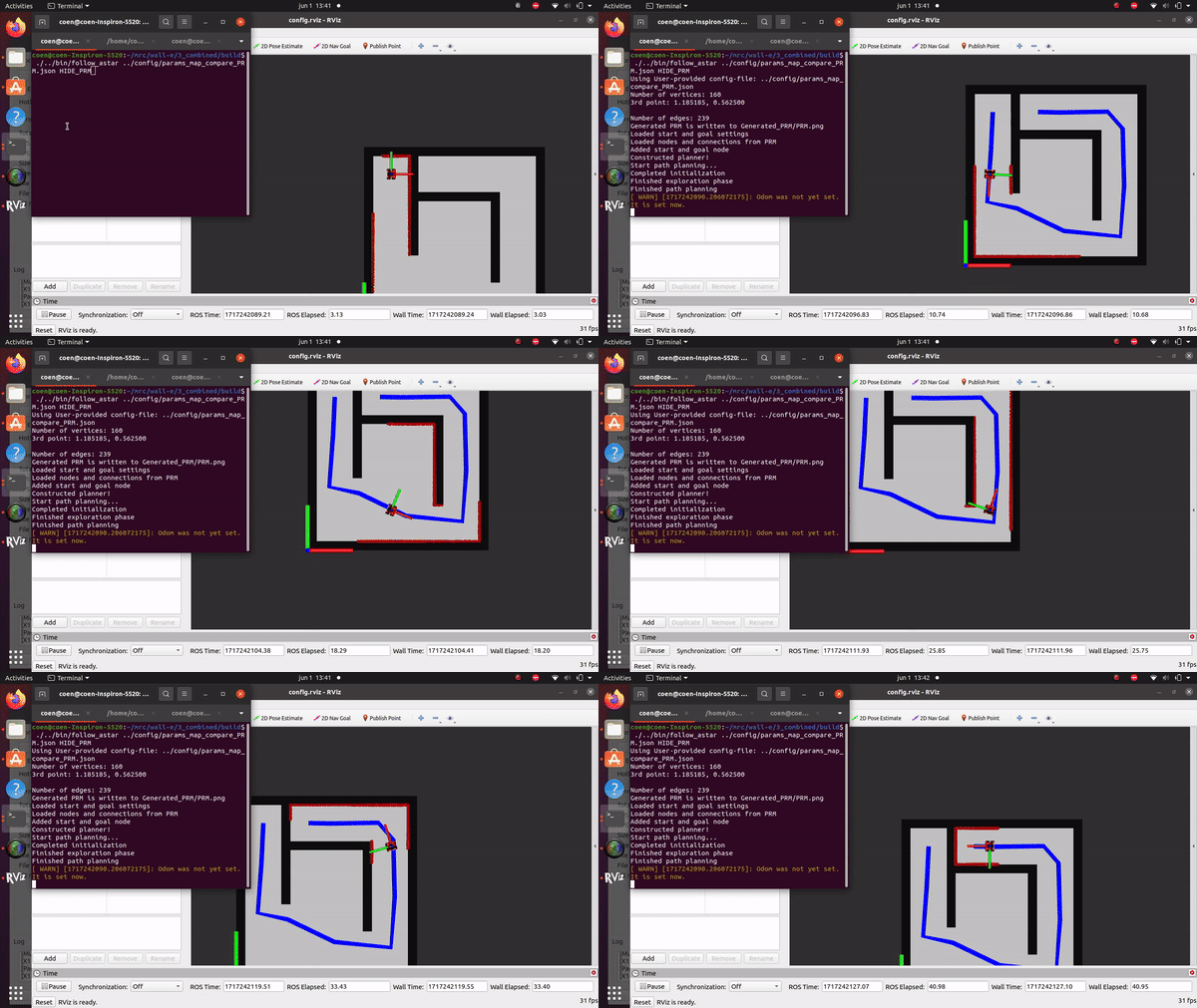
Run the A* algorithm using the gridmap (with the provided nodelist) and using the PRM. What do you observe? Comment on the advantage of using PRM in an open space.

To be added

Localization

Assignment 0.1:

The code is divided into multiple different files, all containing different classes and also a corresponding header file.

Implementation of the Particle Filter initialization.

The particleFilter class

How is the code is structured?

What is the difference between the ParticleFilter and ParticleFilterBase classes, and how are they related to each other?

How are the ParticleFilter and Particle class related to eachother?

Both the ParticleFilterBase and Particle classes implement a propagation method. What is the difference between the methods? Assignment 1.1:

Two constructors, one using a uniform particlespread and one using a Gaussian spread were created.

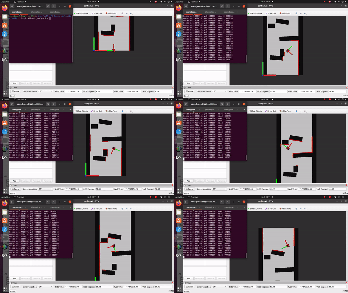
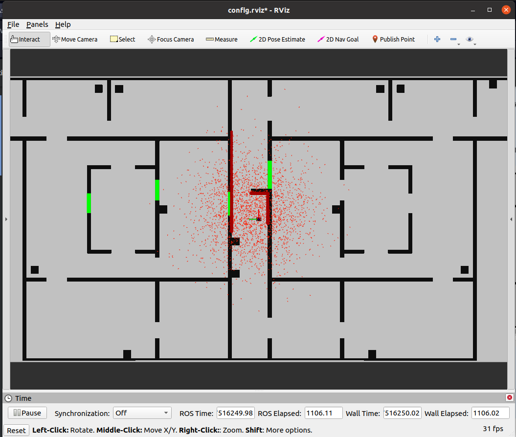
In the case of an initial guess that is fairly accurate a Gaussian distribution ensures that there will be enough samples close to the actual position of the robot. if the initial guess is not accurate, or not known, a uniform distribution is better suited since the entire range is then spanned.The implementation of the particle filter can be seen in the figure on the right

Assignment 1.2:

With the Gaussian particle spread around the initial guess the estimated pose will be placed on this same guess. Since the initial guess is incorrect, the estimated pose is also incorrect.

Using the average pose as the estimated pose is a good method if the predicted particles are close to one another. In the case that multiple clusters form the averaging method will cause the estimated pose to be placed outside of these clusters, the estimated pose will then very likely not be correct. For the final assignment the likelihood of multiple clusters forming is low, since the initial guess is already relatively reliable.

The initialized particle filter can be seen on the right, where a small green arrow is now visible indicating the average and thus estimated pose.

Initialization of the particle filter with the computed average pose.

Assignment 1.3:

The injection of noise in the propagation is necessary to model the uncertainty of the robots odometry data. The noise in propagation ensures that the particles will spread around the uncertain position, ensuring the correct pose is also covered. Without noise in the correction step the predicted posed would slowly divergence from the position of the robot.

The video on the right shows that the estimated position follows the robots movements, indicating the propagation is correctly implemented. Due to the fact that the localization is using no data of the measurements the particles slowly diverge, caused by the random noise that is implemented.

Odometry propagation in the particle filter.

Assignment 2.1:

The measurement model consist of four different components to calculate the probability of a predicted measurement being correct.

- p_hit

This first component calculates a probability of a measurement prediction corresponding to the actual sensor measurement.

- p_short

This represent the probability of the measurement being shorter than the prediction, for example due to an unexpected obstacle being present.. This is necessary in dynamic environments such as the one used for the final assignment.

- p_max

The ' p_max' component incorporates the probability for when no object is detected, which could also happen on non-reflective surfaces.

- p_rand

This last component is uniform over all ranges and accounts for random measurements due to for example noise or errors.

Combining these four forms the final likelihood of a measurement given the expected pose of the robot for a specific ray. For the full range of rays all probabilities are multiplied with one another. For a high number of rays the product will then become incredibly small (since the probability is between 0 and 1). This can cause numerical underflow, where the numbers are too small to accurately represent.

A solution would be to use the log-likelihood of the probability, which is often used in cases like this. Since the number of rays for the final use-case will not be extreme this does not have to be implemented here.

Assignment 2.2:

Two different resampling methods are implemented: Multinomial and Stratified.

- The multinomial method samples according to the weight of the particles, the weight represents the probability that a particle is sampled. This straightforward method In specific situations it might be the case that only higher weight particles are resampled leading to a loss of variance if the same particles keep getting selected. In a situation where these particles are accurately representing the pose of the robot this method is preferred.

- The stratified method subdivides the particles into different groups, in each group particles are resampled. For this method the diversity of the particles is thus guaranteed, also particles with a lower weight are resampled. In situations where the estimated pose is incorrect this method would be preferred.

Assignment 2.3:

Test on the physical model --> TO BE DONE

Explain in a few concise sentences per item:

How you tuned the parameters.

How accurate your localization is, and whether this will be sufficient for the final challenge.

How your algorithm responds to unmodeled obstacles.

Whether your algorithm is sufficiently fast and accurate for the final challenge.

Include a video that shows your algorithm working on the real robot

When finished with the assignments, push the code to your group's git repo