Embedded Motion Control 2014 Group 7: Difference between revisions
| (176 intermediate revisions by 5 users not shown) | |||
| Line 1: | Line 1: | ||
__TOC__ | __TOC__ | ||
= Group members = | |||
{| class="TablePager" style="width: 600px; min-width: 240px; margin-left: 0em; float:left" border="1" cellpadding="5" cellspacing="0" | {| class="TablePager" style="width: 600px; min-width: 240px; margin-left: 0em; float:left" border="1" cellpadding="5" cellspacing="0" | ||
!width="150"|Name | !width="150"|Name | ||
!width=" | !width="400"|Email | ||
!width="150"|ID number | |||
|- | |- | ||
|Maurice van de Ven|| m dot l dot j dot v dot d dot ven @ student dot tue dot nl | |Maurice van de Ven|| m dot l dot j dot v dot d dot ven @ student dot tue dot nl || 0742664 | ||
|- | |- | ||
|Pim Duijsens || p dot j dot h dot duijsens @ student dot tue dot nl | |Pim Duijsens || p dot j dot h dot duijsens @ student dot tue dot nl || 0718473 | ||
|- | |- | ||
|Glenn Roumen || g dot h dot j dot roumen @ student dot tue dot nl | |Glenn Roumen || g dot h dot j dot roumen @ student dot tue dot nl || 0753028 | ||
|- | |- | ||
|Wesley Peijnenburg || w dot peijnenburg @ student dot tue dot nl | |Wesley Peijnenburg || w dot peijnenburg @ student dot tue dot nl || 0790842 | ||
|- | |- | ||
|Roel Offermans || r dot r dot offermans @ student dot tue dot nl | |Roel Offermans || r dot r dot offermans @ student dot tue dot nl || 0656441 | ||
|- | |- | ||
|} | |} | ||
<div style="clear:both"></div> | <div style="clear:both"></div> | ||
= Planning = | |||
<table class="TablePager" style="width: 1200px; min-width: 240px; margin-left: 0em; float:left" border="1" cellpadding="5" cellspacing="0"> | <table class="TablePager" style="width: 1200px; min-width: 240px; margin-left: 0em; float:left" border="1" cellpadding="5" cellspacing="0"> | ||
<tr> | <tr> | ||
<th>Week</th><th>Deadline</th><th>General plan</th><th>Groupmember</th><th>Specific task</th> | <th> Week </th> <th>Deadline</th><th>General plan</th><th>Groupmember</th><th>Specific task</th> | ||
</tr> | </tr> | ||
| Line 33: | Line 34: | ||
<tr> | <tr> | ||
<td> | <td>- - - -</td><td>- - - - -</td><td>- - - - -</td><td>- - - - -</td><td>- - - - -</td> | ||
</tr> | </tr> | ||
| Line 61: | Line 62: | ||
<tr> | <tr> | ||
<td> | <td>- - - -</td><td>- - - - -</td><td>- - - - -</td><td>- - - - -</td><td>- - - - -</td> | ||
</tr> | </tr> | ||
| Line 77: | Line 78: | ||
<tr> | <tr> | ||
<td> | <td>- - - -</td><td>- - - - -</td><td>- - - - -</td><td>- - - - -</td><td>- - - - -</td> | ||
</tr> | </tr> | ||
<tr> | <tr> | ||
<td>7</td><td> | <td>7</td><td>09-06-2014</td><td>Development of modules:</td><td>Cutting corners</td><td>Glenn</td> | ||
</tr> | </tr> | ||
<tr> | <tr> | ||
<td> | <td></td><td>t.b.d.</td><td></td><td>Publishing and listening to arrow</td><td>Wesley/Maurice</td> | ||
</tr> | </tr> | ||
<tr> | <tr> | ||
<td> | <td></td><td>t.b.d.</td><td></td><td>Exploration</td><td>(Pim/Glenn)</td> | ||
</tr> | </tr> | ||
<tr> | <tr> | ||
<td> | <td></td><td>09-06-2014</td><td></td><td>OpenCV - local rectangles solver</td><td>Wesley/Maurice</td> | ||
</tr> | </tr> | ||
<tr> | <tr> | ||
<td>9</td><td>20-06-2014</td><td>Maze Competition</td><td></td><td></td> | <td></td><td>09-06-2014</td><td></td><td>(OpenCV -) floodfill solver</td><td>Roel</td> | ||
</tr> | |||
<tr> | |||
<td>- - - -</td><td>- - - - -</td><td>- - - - -</td><td>- - - - -</td><td>- - - - -</td> | |||
</tr> | |||
<tr> | |||
<td>8</td><td>13-06-2014</td><td>Integration of all nodes</td><td></td><td></td> | |||
</tr> | |||
<tr> | |||
<td>- - - -</td><td>- - - - -</td><td>- - - - -</td><td>- - - - -</td><td>- - - - -</td> | |||
</tr> | |||
<tr> | |||
<td>9</td><td>20-06-2014</td><td>Final presentation of the Maze Strategy and some last improvements</td><td></td><td></td> | |||
</tr> | |||
<tr> | |||
<td>- - - -</td><td>- - - - -</td><td>- - - - -</td><td>- - - - -</td><td>- - - - -</td> | |||
</tr> | |||
<tr> | |||
<td>10</td><td>27-06-2014</td><td>Maze Competition</td><td></td><td></td> | |||
</tr> | </tr> | ||
| Line 104: | Line 130: | ||
<div style="clear:both"></div> | <div style="clear:both"></div> | ||
== | = Corridor strategy = | ||
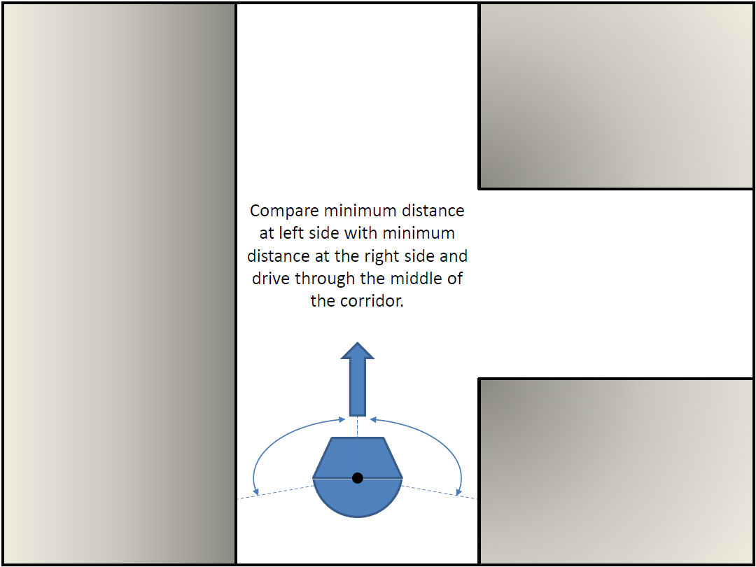
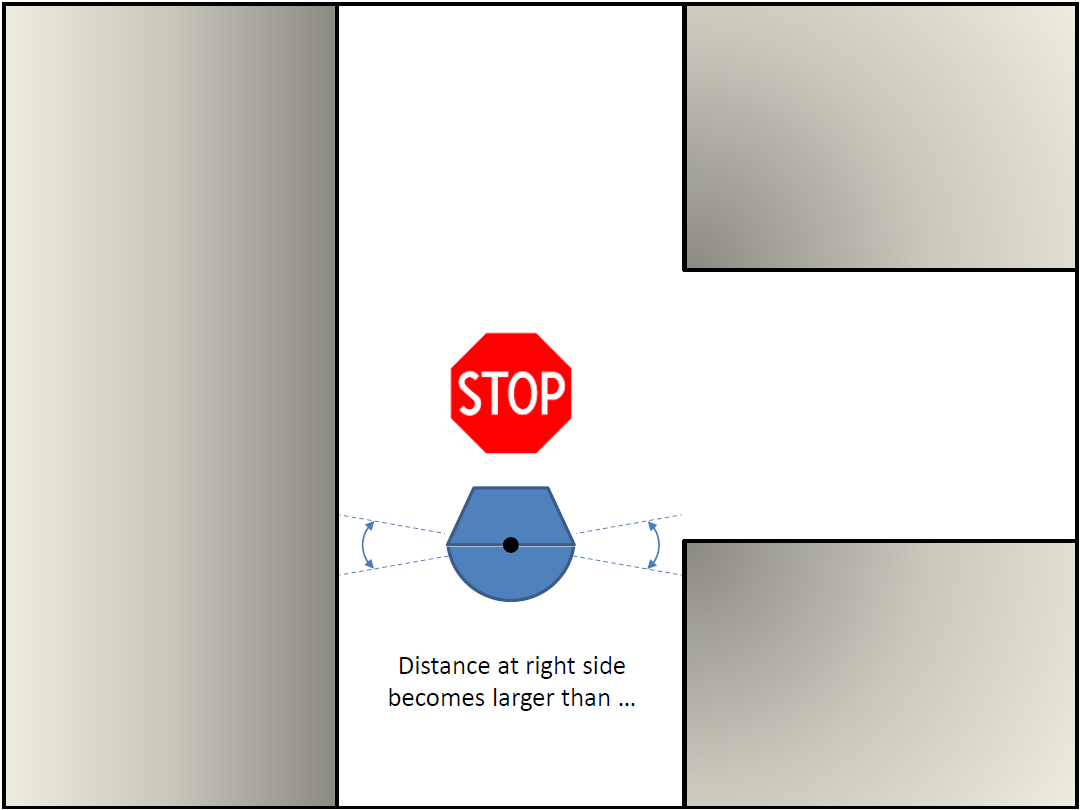
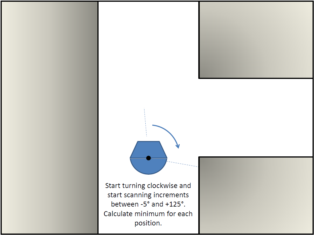
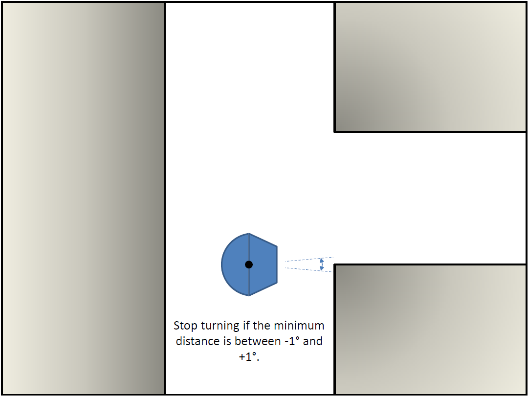
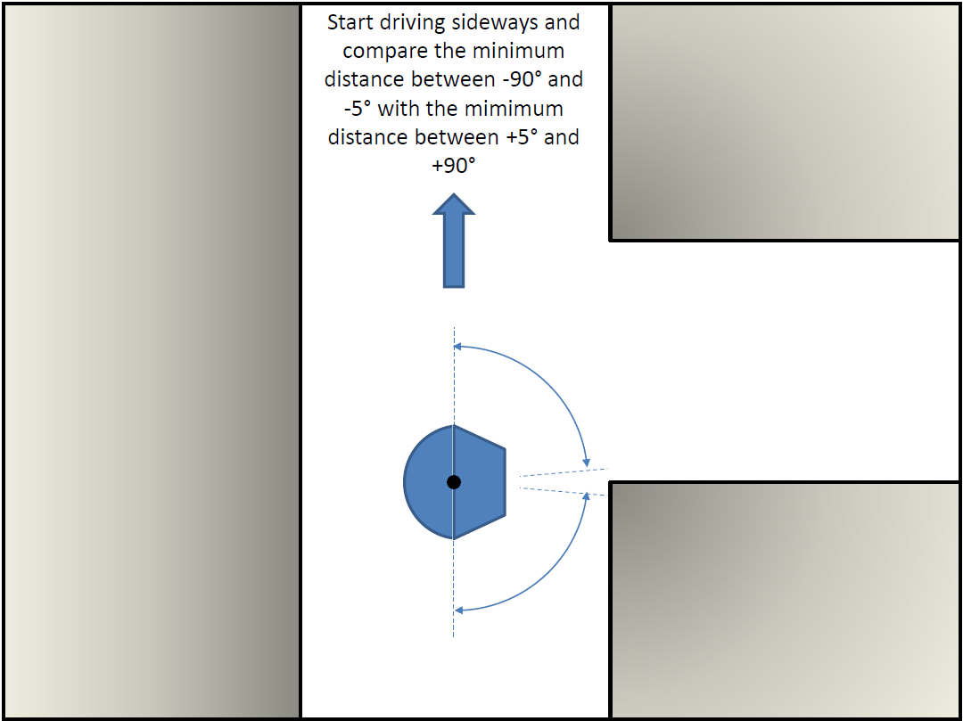
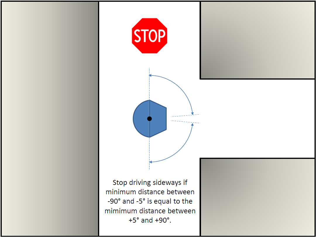
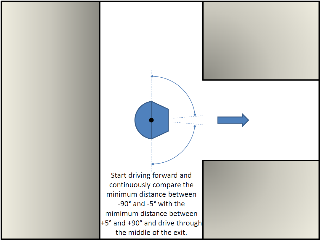
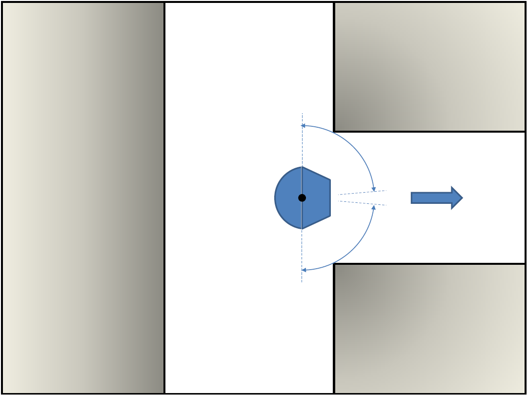
The provided safe_drive file is extended to a file which solves the corridor challenge for a left and right corridor. The strategy, stated below, is implemented and tested. From these tests, it can be concluded that the strategy works properly. Everything is designed and implemented in one single node. The disadvantages of this approach are that it is hard to maintain, hard to extend and teamwork becomes hard. Therefore, it is desired to use different nodes for the maze challenge. | |||
[[File:emc07_2014_pro_cor_step1.png|330px]] [[File:emc07_2014_pro_cor_step2.png|330px]] [[File:emc07_2014_pro_cor_step3.png|330px]] [[File:emc07_2014_pro_cor_step4.png|330px]] | |||
[[File:emc07_2014_pro_cor_step5.png|330px]] [[File:emc07_2014_pro_cor_step6.png|330px]] [[File:emc07_2014_pro_cor_step7.png|330px]] [[File:emc07_2014_pro_cor_step8.png|330px]] | |||
= Maze strategy = | |||
A choice is made to analyze two different approaches to solve the maze challenge. The maze can be solved by using different nodes and design each node from scratch, or by using existing ros packages. If the first method will be chosen, the different nodes and flow chart can be used as stated below. | |||
[[File:scheme_nodes.png|900px|center|alttext|]] | |||
The choice is made to start with using existing ros packages. This is because it is known that ros packages work relatively well for different applications and we thought some packages would be very useful for our case. First, different ros packages are analyzed. The packages GMapping in combination with Move_base are studied and implemented. Since, GMapping and Move_base only covers the mapping, localization and navigation of the pico, a goal planner has to be implemented. The node for the goal planner, the node for the arrow recognition and the integration of both nodes are created from scratch. An alternative for the goal planner is the package Exploration. A more detailed description of the packages and approaches are stated in the next paragraph. The strategy is presented in the diagram below. | |||
[[File:package_overview.png|800px| center]] | |||
== GMapping & Move_base == | |||
'''GMapping''' [http://wiki.ros.org/gmapping link ] | |||
[[File:Gmap2.gif| right]] | |||
GMapping is being investigated as SLAM algorithm. The Pico can, with this simultaneous localization and mapping (SLAM), make a map of an unknown environment and localize itself inside this map. The strategy is to combine the map and the position of the Pico with a navigation stack and a goal planner. GMapping subscribes on /pico/laser and /tf, and publishes on /tf and /map. | |||
In order to run GMapping correctly, a launch file <code>gmap.launch</code> is setup which initializes the correct settings. In this launch file the parameter base_frame is set as /pico/base_link, map_frame as /map and odom_frame as /pico/odom. Also, scan is remapped to /pico/laser. GMapping uses a transform from /map to /pico/odom and vice versa and from /pico/odom to /pico/base_link and vice versa. In order to see how GMapping works, a GIF is presented on the right. The black pixels represent a obstacle, the light gray the known area and the dark gray the unknown area. | |||
<div style="clear:both"></div> | |||
'''Move_base''' [http://wiki.ros.org/move_base link ] | |||
As navigation stack, the move_base-package is used. Move_base provides an action that will attempt to reach a given goal with a mobile base. It makes use of a local and global planner in order to solve a global navigation task. Move_base also maintains a costmap for the global planner and a costmap for the local planner. These costmaps are used to accomplish navigation tasks. | |||
A choice is made to use the base_local_planner inside the move_base stack. From incoming sensor data, angular and linear velocities of the pico are chosen properly by the local planner to traverse the segment of the global path. Trajectory Rollout is used as the local planner. For the global planner, navfn is chosen. This makes use of Dijkstra's algorithm which is explained in the Navigation lecture by J.J.M. Lunenburg. | |||
To launch the move_base stack, again a launch file is created which will initialize the correct settings. The <code>move_base.launch</code> file consists of common settings for both cost maps and separate setting for the global cost map and the local cost map. Also settings for the local planner are set here. Finally is performs a remap from /cmd_vel to /pico/cmd_vel. | |||
The used settings for the costmaps and planner are given below: | |||
{| | |||
!style="text-align:left; width:50%; "| | |||
!style="text-align:left; width:50%; "| | |||
|- valign="top" | |||
|costmap_common_params.yaml: | |||
<pre style="white-space:pre-wrap; width:90%;"> | |||
transform_tolerance: 0.4 | |||
obstacle_range: 2.5 | |||
raytrace_range: 3.0 | |||
inflation_radius: 0.30 | |||
robot_radius: 0.25 | |||
observation_sources: laser_scan_sensor | |||
laser_scan_sensor: {sensor_frame: pico/laser, data_type: LaserScan, topic: /pico/laser, marking: true, clearing: true} | |||
</pre> | |||
|rowspan="3"|base_local_planner_params.yaml | |||
<pre style="white-space:pre-wrap; width:90%;"> | |||
TrajectoryPlannerROS: | |||
acc_lim_x: 2.5 | |||
acc_lim_y: 2.5 | |||
acc_lim_theta: 3.2 | |||
max_vel_x: 0.2 | |||
min_vel_x: 0.0 | |||
max_vel_theta: 1.0 | |||
min_vel_theta: -1.0 | |||
min_in_place_vel_theta: 1.0 | |||
escape_vel: -0.2 | |||
holomonic_robot: true | |||
y_vels: -0.2, -0.0, 0.0, 0.2 | |||
yaw_goal_tolerance: 0.05 | |||
xy_goal_tolerance: 0.10 | |||
latch_xy_goal_tolerance: false | |||
sim_time: 2.0 | |||
sim_granularity: 0.005 | |||
angular_sim_granularity: 0.025 | |||
vx_samples: 5 | |||
vtheta_samples: 10 | |||
meter_scoring: true | |||
pdist_scale: 2.0 | |||
gdist_scale: 1.0 | |||
occdist_scale: 0.05 | |||
heading_lookahead: 0.325 | |||
heading_scoring: false | |||
heading_scoring_timestep: 0.8 | |||
dwa: false | |||
publish_cost_grid_pc: false | |||
global_frame_id: /pico/odom | |||
</pre> | |||
|- | |||
|global_costmap_params.yaml: | |||
<pre style="white-space:pre-wrap; width:90%;"> | |||
global_costmap: | |||
global_frame: /map | |||
robot_base_frame: /pico/base_link | |||
update_frequency: 5.0 | |||
static_map: true | |||
publish_frequency: 2.0 | |||
</pre> | |||
|- | |||
|local_costmap_params.yaml: | |||
<pre style="white-space:pre-wrap; width:90%;"> | |||
local_costmap: | |||
global_frame: /pico/odom | |||
robot_base_frame: /pico/base_link | |||
update_frequency: 5.0 | |||
publish_frequency: 2.0 | |||
static_map: false | |||
rolling_window: true | |||
width: 3.0 | |||
height: 3.0 | |||
resolution: 0.05 | |||
</pre> | |||
|} | |||
When a goal is given in Cartesian coordinates, move_base navigates and publishes on /pico/cmd_vel to reach that goal, if it is possible. This is presented in the figures stated below. Move_base creates an inflated radius around the Pico and an inflated radius around the obstacle pixels from GMapping. When the radii are set to the correct values, the Pico will not hit any obstacles according to move_base. When it is not possible for the Pico to reach the given goal, move_base goes into a recovery mode until the goal becomes reachable due to new map data obtained from the recovery or it is given a different goal. | |||
[[File:Move base07.png|800px| center]] | |||
<div style="clear:both"></div> | |||
An issue with move_base is, that it will not move to its first goal when given by the goal planner. After a given time, the Pico will go to a recovery mode and starts moving to its goal. The recovery mode is not desired in the beginning because of placing an arc in OpenCv, as will be explained in the next paragraph. Therefore the Pico will be initialized by a velocity command in the x-direction. The map will update again and Pico drives to its first goal. | |||
While GMapping and move_base are running, a tf tree can be made to see how the different frames are linked. For the chosen settings of GMapping and move_base, this results in the following scheme: | |||
[[File:tftree_movebase2.png|center]] | |||
== Exploration == | |||
'''Explore_stage''' | |||
An existing package which works as a goal planner, SLAM and navigation stack, is the explore_stage package. This package is an algorithm that interacts with GMapping to create a map to find exits and tries to navigate by launching a node in Move_base. Which is useful in maze solving case. In order to start this package, again a launch file is made. The same local and global costmap settings have been used as in the previous packages. | |||
The following problems occur: when using RVIZ, it can be seen that a path is planned to an exit, but most of the time the pico seems stuck. Also, when defining a new goal manually by RVIZ, it repeats saying that a node is added on the coordinates: X.X and X.X but the pico does nothing. It also repeats the following warning: Entropy has not been updated. Loop closure opportunities may be ignored. | |||
Within the given time limit, it was not possible to make the Explore_stage package work as desired. The choice is made to continue with GMapping and Move_base in addition with a goal_planner and arrow recognition created from scratch. | |||
== Goal planning - OpenCV == | |||
The goal planner makes use of different messages and data types. The most important messages and data types which form the basis of the goal planner algorithm are given below. | |||
{| class="TablePager" border="1" cellpadding="5" cellspacing="0" | {| class="TablePager" style="width: 600px; min-width: 240px; margin-left: 0em; float:left" border="1" cellpadding="5" cellspacing="0" | ||
!width=" | !width="200"|Datatype | ||
!width=" | !width="400"|Purpose | ||
|- | |||
|[http://docs.ros.org/api/nav_msgs/html/msg/Odometry.html Odometry] | |||
| Odometry data from pico | |||
|- | |- | ||
| | |[http://docs.ros.org/api/nav_msgs/html/msg/OccupancyGrid.html OccupancyGrid] | ||
| Map data generated by Gmapping stored in a vector | |||
|- | |- | ||
| | |[http://docs.ros.org/api/nav_msgs/html/msg/MapMetaData.html MapMetaData] | ||
| Map information such as resolution and position of origin | |||
|- | |- | ||
| | |[http://docs.ros.org/api/sensor_msgs/html/msg/LaserScan.html LaserScan] | ||
| Laser data | |||
|- | |- | ||
| | |[http://docs.ros.org/electric/api/move_base_msgs/html/MoveBaseActionFeedback_8h.html MoveBaseActionFeedback] | ||
| Position and orientation from Pico | |||
|- | |- | ||
| | |[http://docs.ros.org/electric/api/move_base_msgs/html/MoveBaseAction_8h.html MoveBaseAction] | ||
| Allows publishing a goal to move_base | |||
|- | |- | ||
|} | |||
<div style="clear:both"></div> | |||
'''Strategy''' | |||
The strategy of the goal planner is chosen to be frontier based. The idea is that the destination goals of the pico are set around the lines between known and unknown area. This can be seen as an explorer which tells pico to explore all unknown areas. This is done with OpenCV by subscribing on the /Map topic on which a matrix/image of a map is published by GMapping. With some tools of the OpenCV library, this image of a map is processed in order to publish Cartesian coordinates to Move_base as a goal. Since, GMapping updates the map in time, new goals are set every time a map is updated. When multiple goals are given, the closest goal to pico is chosen as the primary goal. The choice of the correct primary goal will change when an arrow is detected. This will be explained in the next paragraph. | |||
To retrieve goals from the map data the following steps are implemented: | |||
1: | |||
The laser data is converted to an image which can be processed using OpenCV. The laser data is provided as a vector in which the walls have a value of 100, the known area have a value of 1 and the unknown area have a value of 0. In the generated picture the walls are colored black, the known area white and the unknown area grey. | |||
2: | |||
All black pixels are inflated using a circle of a certain radius depending on the inflation radius chosen in the move_base. The color of the (remaining) known area is changed to red. | |||
3: | |||
All pixels of the unknown area (gray) which neighbor known area (red) are inflated by a square. This inflation is implemented to filter noise and remove areas which are unreachable. Next, all boundaries between known and unknown area are colored green. | |||
4: | |||
A binary is created for the green pixels only. This binary input is used to detect lines. The line detection is done by a [http://docs.opencv.org/doc/tutorials/imgproc/imgtrans/hough_lines/hough_lines.html hough line transform]. The midpoint of each line will be set a provisional goal. | |||
5: | |||
Each goal will be evaluated for reachability. To check this, a floodfill (pink) with Pico as starting point is used. The entry of the maze is closed with an ellipse so no goals will be found at the entry of the maze. All goals lying in the floodfilled area are considered as valid goal targets. Goals which do not lie in the flooded area are discarded. | |||
6: At this point multiple valid goals are available but only one goal can be used as a goal to drive to. First the closest goal in front of pico is given priority. If there are no valid goals in front of pico, the closest goal behind pico will be chosen. | |||
The image below shows the map processing for goal planning in several steps. | |||
[[File:goal_planner.jpg|center]] | |||
During the developing of the goal planner several issues occurred and are solved. | |||
An issue occurs when there are a few laser beams passing through a hole in the wall or just around a corner. It is possible that a goal is set at the frontier of these few laser beams. Since it is not possible for pico to reach these goals, pico will go to its recovery mode. To solve this problem, a floodfill algorithm is used. Unknown area will be inflated and the area starting from pico will be floodfilled. The remaining area is seen as the known area. This way, unreachable areas will be filtered. This can be seen in the pictures given below. The pink area in the right figure is the floodfilled area. | |||
[[File:Floodfill07.png|center]] | |||
Another issue is the area behind pico at start, which will be seen as a frontier. It is therefore possible that the goal planner sets its goal to the start and tries to reach the unknown area. This problem is solved by adding an arc behind the starting position of pico in the OpenCV images which closes the entrance. Therefore no goal will be set at this position. | |||
Also an issue occurs when there is a frontier near a wall which is not detected by the laser data yet. The goal will be set near this the wall and the pico will not be able to reach this goal, as it is inside the inflated area as soon as pico has detected the wall. This problem is solved by inflating the unknown area. The goal will be set with an offset from the frontier. This problem was also solved by the fact that GMapping updates its map. The pico will see the wall when it moves towards the goal and a new goal will be set. However, if it takes too much time to update the map and process the data, this map updating would not solve the problem. | |||
'''Recovery mode''' | |||
If no valid goals are found, no path can be planned to a goal. Therefore pico will not move and no new goals will be planned. In this situation pico is stuck and a recovery is needed. If pico does not move for a certain time, the recovery mode will be initialized. First it is checked depending on the laser data if pico can move forward. If this is not possible Pico will rotate at his current position. Moving forward or rotating causes gmapping to update the map. From the updated map new valid goals can be found. | |||
'''Initialization''' | |||
At the startup, the goal planner does not recieve enough information to plan a valid goal point. Information such as the map and pico's orientation are not received yet. In order to get all the necessary data, pico first needs to move. Therefore an initialization is integrated. In this integration pico will move forward for 0.5m. By moving forward all the necessary information will be received by the goal planner and the normal algorithm as described above will provide pico with new goal points. | |||
<div style="clear:both"></div> | |||
== Arrow recognition - OpenCV == | |||
''' Strategy ''' | |||
The arrow detection node will publish alongside the goal planner node. The idea is to process the image of the camera in the following way: the image of the camera is converted from red-green-blue (RGB) to hue-saturation-value (HSV) (picture 1). A double for-loop is used to convert every red-tinted pixel to black. A binary (two-colour) image is created based on the black and non-black colours (picture 2). This image is then blurred and an edge detection algorithm gives an output of the edges that it can find (picture 3). | |||
[[File:emc07_Arrow_recognition_alg.png|1000px|center]] | |||
The list of edges is the basis for the arrow recognition, all lines are defined from left to right (so: x1 < x2). Lines are defined as follows: Vec4i line[x1,y1,x2,y2]. The lines are filtered, and the ones that remain are lines with a slope of +/-30 with a +/- 5 degrees margin. All lines with a negative slope are compared with all lines that have a positive slope. Both the +30 [deg] and the -30 [deg] line have a beginning and end point. If the left (begin) points are close enough to each other (3 pixels), the output is "LEFT ARROW", and vice versa. The arrow detection node publishes 0 when no arrow is found and -1 and 1 for the left and right arrow respectively. | |||
The image below shows the +/-30 [deg] lines which this algorithm focuses on: | |||
[[File:EMC07_-_arrow.png|600px|center]] | |||
= Integration = | |||
An integration plan is necessary for the nodes to communicate properly and produce meaningful results. The following nodes needed to be linked: | |||
- GMapping; | |||
- Move_base; | |||
- Arrow recognition; | |||
- Goal planner. | |||
Using <code>rqt_graph</code>, the following graph is given: | |||
[[File:Rosgraph92.png|1400px]] | |||
The picture above describes the nodes that are communicating and the topics that they use. Both Move_base and GMapping already incorporate important aspects such as the laserdata and internal communication. Both the goal planner and arrow recognition script are self made and needed manual integration of the following aspects: | |||
- Retrieve map data in goal planner; | |||
- Retrieve image data in the arrow recognition; | |||
- Send the arrow direction to the goal planner; | |||
- Retrieve arrow direction in the goal planner; | |||
- Combine possible goal locations with arrow input and send a simple goal to Move_base; | |||
- When there are no goals, send a recovery goal to refresh the map and find new pathways. | |||
Two of the big challenges in the goal planner are the conversion of the map to a useful image and the decision making in case of arrow input. The animated picture below shows the simulation where Pico is given the "arrow right" input by playing a bag file on the background. This is where Pico is forced to make a decision. | |||
[[File:arrowgif.gif|arrowgif.gif]] | |||
Explanation of the picture: | |||
- White cross = location of Pico; | |||
- Purple line = looking direction of Pico; | |||
- Other white lines from Pico's location = Pico's field of view (Goals in front have high priotity); | |||
- Green lines from Pico's location = Pico's field of view with arrow input (Goals to the right or left have high priority); | |||
- Yellow line = The direction Pico would choose without arrow input. | |||
The picture clearly shows that Pico is ignoring the goals that it would otherwise head for. Pico is choosing the direction that the arrow is pointing towards. | |||
= Results = | |||
{| | |||
!style="text-align:left; width:50%; "| Corridor challenge: | |||
!style="text-align:left; width:50%; "| Simulation 1: | |||
|- valign="top" | |||
|[[File:filmintro_corridor_play.jpg|400px|left|link=https://www.youtube.com/watch?v=EBLNCvvevCU]] | |||
|[[File:filmintro3_play.jpg|400px|left|link=https://www.youtube.com/watch?v=oW0filHJpZY]] | |||
|} | |||
{| | |||
!style="text-align:left; width:50%; "| Simulation 2: | |||
!style="text-align:left; width:50%; "| Maze challenge: | |||
|- valign="top" | |||
|[[File:filmintro_simulation_play.jpg|400px|left|link=https://www.youtube.com/watch?v=YP00LAQkX0M]] | |||
|[[File:filmintro_maze_play.jpg|400px|left|link=https://www.youtube.com/watch?v=1VOEbYB-t4s]] | |||
|} | |} | ||
== Time Table | |||
<div style="clear:both"></div> | |||
= Evaluation = | |||
The maze competition was passed within 2 minutes and 40 seconds. As seen in the video of the maze competition, Pico had problems passing the second crossing with two dead ends. This has cost us a lot of time, but Pico was able to unstuck itself thanks to its built-in recovery mode. | |||
Previous practical tests have shown that Pico can find any exit in a much shorter timespan. At the moment it is not certain what exactly went wrong. A potential cause could be a flaw in the goal planner node which slows down the script. Another problem during the competition was that the GMapping script was consuming an unusually high amount of processor power. | |||
For the maze competition with a relative simple structure (straight corridors, perpendicular corners and easy to detect deadends), our approach was at disadvantage because of complexity. A properly working case-detector could have been faster. Our solution would have a big advantage in a complex maze, with non-rectangular shapes and narrow passings included. Pico would be able to plan goals and move towards them in order to explore the whole area and eventually solve the maze. | |||
The disadvantages of the chosen solution: | |||
- A time consuming (inefficient) goal planner script; | |||
- A complex solution for a relatively simple challenge. | |||
The advantages: | |||
- Reliability, the robot will only stop if everything is explored and remaining goals are unreachable; | |||
- Can solve any maze, strange shapes or too narrow pathways don't influence the resolvability; | |||
- Can recognise dead ends and moves on to look for alternatives. | |||
= Practical issues = | |||
''' TF tree ''' | |||
Viewing a tf tree can be done by: | |||
<pre>$ rosrun tf view_frames</pre> | |||
''' GMapping and Move_base in simulations ''' | |||
1. Start Gazebo: | |||
<pre>$ gazebo </pre> | |||
2. Using another terminal, spawn the maze: | |||
<pre>$ rosrun gazebo_map_spawner spawn_maze </pre> | |||
3. Launch PICO: | |||
<pre>$ roslaunch pico_gazebo pico.launch </pre> | |||
4. Start RViz to visualize how PICO perceives the world through its sensors. | |||
<pre>$ rosrun pico_visualization rviz </pre> | |||
5. Launch the gmapping plugin for PICO | |||
<pre>$ roslaunch pico_2ndnav gmap.launch </pre> | |||
6. Launch the move_base package for PICO to navigate through the maze with the preferred settings. | |||
<pre>$ roslaunch pico_2ndnav move_base.launch </pre> | |||
''' Explore_stage in simulations ''' | |||
1. Get in the right directory: | |||
<pre>$ roscd explore_stage </pre> | |||
2. Launch the explore_stage launch file: | |||
<pre>$ roslaunch explore_slam.launch </pre> | |||
''' Goal planning - OpenCV ''' | |||
In some cases, your script will not find the required include: | |||
<pre> | |||
#include <move_base_msgs/MoveBaseActionFeedback.h> // Contains the location of pico | |||
</pre> | |||
The solution (ubuntu command): | |||
<pre> | |||
sudo cp -a /opt/ros/groovy/stacks/navigation/move_base_msgs/msg_gen/cpp/include/. /opt/ros/groovy/include/ | |||
</pre> | |||
The OpenCV C++ files can be compiled using one of the given commands below. For the g++ command, the packages need to be specified manually. | |||
<pre>$ g++ demo_opencv.cpp `pkg-config opencv --cflags --libs` -o demo_opencv </pre> | |||
Or you can make have ROS find the libaries for you: | |||
<pre>$ rosmake demo_opencv </pre> | |||
Executing the program: | |||
<pre>$ ./demo_opencv <argcount> <arg(s)> </pre> | |||
''' Goal planning - OpenCV Troubleshooting ''' | |||
There have been problems with the OpenCV and Highgui libraries (static libraries). This problem can be solved by replacing the following code: | |||
<pre> | |||
// #include "cv.h" // (commented out) | |||
#include "opencv2/opencv.hpp" | |||
// #include <highgui.h> // (commented out) | |||
#include <opencv/highgui.h> | |||
</pre> | |||
The program might not always respond to input, this is can be due to a subscription to the wrong topic. Make sure you are streaming the images and check the ros-topic with: | |||
<pre> rostopic list </pre> | |||
Then the output gives "/pico/camera", "/pico/asusxtion/rgb/image_color", or a different name. Replace the referece in the following line of code: | |||
<pre> ros::Subscriber cam_img_sub = nh.subscribe("/pico/asusxtion/rgb/image_color", 1, &imageCallback); </pre> | |||
'''Runnig OpenCV on an image stream from a bag file:''' | |||
In three separate terminals: | |||
<pre> | |||
roscore | |||
rosbag play <location of bag file> | |||
./demo_opencv | |||
</pre> | |||
''' Arrow recognition ''' | |||
The image is cropped using: | |||
<pre> | |||
cv::Rect myROI(120,220,400,200); // Rect_(x,y,width,height) | |||
cv::Mat croppedRef(img_rgb, myROI); // The window is 480 rows and 640 cols | |||
</pre> | |||
''' Pico experiment setup ''' | |||
Terminal 1: | |||
<pre style="white-space:pre-wrap; width:30%;"> | |||
ssh pico | |||
pico123 | |||
pstart | |||
</pre> | |||
Terminal 2: | |||
<pre style="white-space:pre-wrap;width:30%;"> | |||
pico-core | |||
rviz rviz | |||
</pre> | |||
Terminal 3: | |||
<pre style="white-space:pre-wrap;width:30%;"> | |||
ssh pico | |||
pico123 | |||
roscd gmapping | |||
**check if group 11 has gmapping if so delete gmapping map** | |||
cd .. | |||
rm -rf gmapping | |||
cd ros/groovy/emc/groups/emc07 | |||
svn up | |||
roscd pico_2ndnav | |||
roslaunch pico_2ndnav gmap.launch | |||
</pre> | |||
Terminal 4: | |||
<pre style="white-space:pre-wrap;width:30%;"> | |||
ssh pico | |||
pico123 | |||
roscd pico_2ndnav | |||
roslaunch pico_2ndnav move_base.launch | |||
</pre> | |||
Terminal 5: | |||
<pre style="white-space:pre-wrap;width:30%;"> | |||
ssh pico | |||
pico123 | |||
roscd goal_planner_roel2 | |||
rosmake goal_planner_roel2 | |||
./bin/goal_xtc | |||
</pre> | |||
Terminal 6: | |||
<pre style="white-space:pre-wrap;width:30%;"> | |||
ssh pico | |||
pico123 | |||
roscd demo_opencv_wesley | |||
rosmake demo_opencv_wesley | |||
./bin/demo_xtc | |||
</pre> | |||
= Time Table = | |||
{| border="1" class="TablePager" cellpadding="3" cellspacing="0" | {| border="1" class="TablePager" cellpadding="3" cellspacing="0" | ||
| Line 184: | Line 716: | ||
|- | |- | ||
! Maurice | ! Maurice | ||
| | | 2|| 3 || 10 || 4 || || || | ||
|- | |- | ||
! Wesley | ! Wesley | ||
| Line 202: | Line 734: | ||
|- | |- | ||
! Maurice | ! Maurice | ||
| ||5 || ||15 || || || | | 2||5 || ||15 || || || | ||
|- | |- | ||
! Wesley | ! Wesley | ||
| Line 217: | Line 749: | ||
|- | |- | ||
! Roel | ! Roel | ||
| | | 2 || 2.5 || || ||6 || || 1 | ||
|- | |- | ||
! Maurice | ! Maurice | ||
| 2 || 2.5|| || || 8|| || | | 2 || 2.5|| || || 8||0.5 || | ||
|- | |- | ||
! Wesley | ! Wesley | ||
| Line 232: | Line 764: | ||
|- | |- | ||
! Pim | ! Pim | ||
| || | | || 4 || || || 6 || || | ||
|- | |- | ||
! Roel | ! Roel | ||
| || | | || 4 || || || 6 || || | ||
|- | |- | ||
! Maurice | ! Maurice | ||
| || || || || || || | | ||4 || || || 8|| || | ||
|- | |- | ||
! Wesley | ! Wesley | ||
| | | || 4 || 8 || || 14 || || | ||
|- | |- | ||
! Glenn | ! Glenn | ||
| || | | || 4 || || || 8 || 1 || | ||
|- | |- | ||
== | | colspan="8" style="text-align: center;"| Week 7 | ||
|- | |||
! Pim | |||
| 2 || 2.5 || || || 10 || || | |||
|- | |||
! Roel | |||
| 2 || 4 || || || 8 || || 3 | |||
|- | |||
! Maurice | |||
| 2 ||4 || || ||9 ||2 || | |||
|- | |||
! Wesley | |||
| 2 || 4 || 2 || || 12 || || | |||
|- | |||
! Glenn | |||
| 2 || 2 || || || 8 || 5 || | |||
|- | |||
| colspan="8" style="text-align: center;"| Week 8+9 | |||
|- | |||
! Pim | |||
| 4 || 1.5 || || || 23 || || | |||
|- | |||
! Roel | |||
| || 2.5 || || || 20 || || 4 | |||
|- | |||
! Maurice | |||
| || 0.5|| || || 20|| 2||4 | |||
|- | |||
! Wesley | |||
| || 0.5 || || || 29 || || | |||
|- | |||
! Glenn | |||
| || || || || 10 || 5 || | |||
|- | |||
|} | |||
2 | |||
4 | |||
Latest revision as of 19:21, 2 July 2014
Group members
| Name | ID number | |
|---|---|---|
| Maurice van de Ven | m dot l dot j dot v dot d dot ven @ student dot tue dot nl | 0742664 |
| Pim Duijsens | p dot j dot h dot duijsens @ student dot tue dot nl | 0718473 |
| Glenn Roumen | g dot h dot j dot roumen @ student dot tue dot nl | 0753028 |
| Wesley Peijnenburg | w dot peijnenburg @ student dot tue dot nl | 0790842 |
| Roel Offermans | r dot r dot offermans @ student dot tue dot nl | 0656441 |
Planning
| Week | Deadline | General plan | Groupmember | Specific task |
|---|---|---|---|---|
| 4 | 16-05-2014 | Complete Corridor Challenge | ||
| - - - - | - - - - - | - - - - - | - - - - - | - - - - - |
| 5 | 19-05-2014 | Research Maze Strategies and define modules | ||
| 19-05-2014 before 10:45 h. | Roel | Research possibilities for wall and corner detection with OpenCV | ||
| 19-05-2014 before 10:45 h. | Glenn | Research possibilities for wall and corner detection with OpenCV | ||
| 19-05-2014 before 10:45 h. | Wesley | Research possibilities for arrow detection with OpenCV | ||
| 19-05-2014 before 10:45 h. | Maurice | Research possibilities for path planning and path tracker/driver | ||
| 19-05-2014 before 10:45 h. | Pim | Research possibilities for path planning and path tracker/driver | ||
| - - - - | - - - - - | - - - - - | - - - - - | - - - - - |
| 6 | 26-05-2014 | Research functionality of ROS Packages: Gmapping and move_base | ||
| 28-05-2014 | Decide: use of packages or write complete new code | |||
| 30-05-2014 | Conceptual version of all modules are finished | |||
| - - - - | - - - - - | - - - - - | - - - - - | - - - - - |
| 7 | 09-06-2014 | Development of modules: | Cutting corners | Glenn |
| t.b.d. | Publishing and listening to arrow | Wesley/Maurice | ||
| t.b.d. | Exploration | (Pim/Glenn) | ||
| 09-06-2014 | OpenCV - local rectangles solver | Wesley/Maurice | ||
| 09-06-2014 | (OpenCV -) floodfill solver | Roel | ||
| - - - - | - - - - - | - - - - - | - - - - - | - - - - - |
| 8 | 13-06-2014 | Integration of all nodes | ||
| - - - - | - - - - - | - - - - - | - - - - - | - - - - - |
| 9 | 20-06-2014 | Final presentation of the Maze Strategy and some last improvements | ||
| - - - - | - - - - - | - - - - - | - - - - - | - - - - - |
| 10 | 27-06-2014 | Maze Competition |
Corridor strategy
The provided safe_drive file is extended to a file which solves the corridor challenge for a left and right corridor. The strategy, stated below, is implemented and tested. From these tests, it can be concluded that the strategy works properly. Everything is designed and implemented in one single node. The disadvantages of this approach are that it is hard to maintain, hard to extend and teamwork becomes hard. Therefore, it is desired to use different nodes for the maze challenge.
Maze strategy
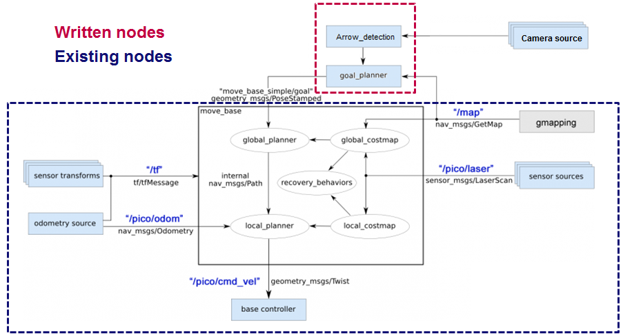
A choice is made to analyze two different approaches to solve the maze challenge. The maze can be solved by using different nodes and design each node from scratch, or by using existing ros packages. If the first method will be chosen, the different nodes and flow chart can be used as stated below.

The choice is made to start with using existing ros packages. This is because it is known that ros packages work relatively well for different applications and we thought some packages would be very useful for our case. First, different ros packages are analyzed. The packages GMapping in combination with Move_base are studied and implemented. Since, GMapping and Move_base only covers the mapping, localization and navigation of the pico, a goal planner has to be implemented. The node for the goal planner, the node for the arrow recognition and the integration of both nodes are created from scratch. An alternative for the goal planner is the package Exploration. A more detailed description of the packages and approaches are stated in the next paragraph. The strategy is presented in the diagram below.
GMapping & Move_base
GMapping link
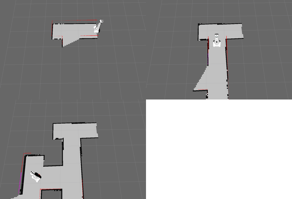
GMapping is being investigated as SLAM algorithm. The Pico can, with this simultaneous localization and mapping (SLAM), make a map of an unknown environment and localize itself inside this map. The strategy is to combine the map and the position of the Pico with a navigation stack and a goal planner. GMapping subscribes on /pico/laser and /tf, and publishes on /tf and /map.
In order to run GMapping correctly, a launch file gmap.launch is setup which initializes the correct settings. In this launch file the parameter base_frame is set as /pico/base_link, map_frame as /map and odom_frame as /pico/odom. Also, scan is remapped to /pico/laser. GMapping uses a transform from /map to /pico/odom and vice versa and from /pico/odom to /pico/base_link and vice versa. In order to see how GMapping works, a GIF is presented on the right. The black pixels represent a obstacle, the light gray the known area and the dark gray the unknown area.
Move_base link
As navigation stack, the move_base-package is used. Move_base provides an action that will attempt to reach a given goal with a mobile base. It makes use of a local and global planner in order to solve a global navigation task. Move_base also maintains a costmap for the global planner and a costmap for the local planner. These costmaps are used to accomplish navigation tasks.
A choice is made to use the base_local_planner inside the move_base stack. From incoming sensor data, angular and linear velocities of the pico are chosen properly by the local planner to traverse the segment of the global path. Trajectory Rollout is used as the local planner. For the global planner, navfn is chosen. This makes use of Dijkstra's algorithm which is explained in the Navigation lecture by J.J.M. Lunenburg.
To launch the move_base stack, again a launch file is created which will initialize the correct settings. The move_base.launch file consists of common settings for both cost maps and separate setting for the global cost map and the local cost map. Also settings for the local planner are set here. Finally is performs a remap from /cmd_vel to /pico/cmd_vel.
The used settings for the costmaps and planner are given below:
costmap_common_params.yaml:
  transform_tolerance: 0.4
  obstacle_range: 2.5
  raytrace_range: 3.0
  inflation_radius: 0.30
  robot_radius: 0.25
  observation_sources: laser_scan_sensor
  laser_scan_sensor: {sensor_frame: pico/laser, data_type: LaserScan, topic: /pico/laser, marking: true, clearing: true}
|
base_local_planner_params.yaml
TrajectoryPlannerROS: acc_lim_x: 2.5 acc_lim_y: 2.5 acc_lim_theta: 3.2 max_vel_x: 0.2 min_vel_x: 0.0 max_vel_theta: 1.0 min_vel_theta: -1.0 min_in_place_vel_theta: 1.0 escape_vel: -0.2 holomonic_robot: true y_vels: -0.2, -0.0, 0.0, 0.2 yaw_goal_tolerance: 0.05 xy_goal_tolerance: 0.10 latch_xy_goal_tolerance: false sim_time: 2.0 sim_granularity: 0.005 angular_sim_granularity: 0.025 vx_samples: 5 vtheta_samples: 10 meter_scoring: true pdist_scale: 2.0 gdist_scale: 1.0 occdist_scale: 0.05 heading_lookahead: 0.325 heading_scoring: false heading_scoring_timestep: 0.8 dwa: false publish_cost_grid_pc: false global_frame_id: /pico/odom |
global_costmap_params.yaml:
global_costmap: global_frame: /map robot_base_frame: /pico/base_link update_frequency: 5.0 static_map: true publish_frequency: 2.0 | |
local_costmap_params.yaml:
local_costmap: global_frame: /pico/odom robot_base_frame: /pico/base_link update_frequency: 5.0 publish_frequency: 2.0 static_map: false rolling_window: true width: 3.0 height: 3.0 resolution: 0.05 |
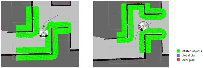
When a goal is given in Cartesian coordinates, move_base navigates and publishes on /pico/cmd_vel to reach that goal, if it is possible. This is presented in the figures stated below. Move_base creates an inflated radius around the Pico and an inflated radius around the obstacle pixels from GMapping. When the radii are set to the correct values, the Pico will not hit any obstacles according to move_base. When it is not possible for the Pico to reach the given goal, move_base goes into a recovery mode until the goal becomes reachable due to new map data obtained from the recovery or it is given a different goal.
An issue with move_base is, that it will not move to its first goal when given by the goal planner. After a given time, the Pico will go to a recovery mode and starts moving to its goal. The recovery mode is not desired in the beginning because of placing an arc in OpenCv, as will be explained in the next paragraph. Therefore the Pico will be initialized by a velocity command in the x-direction. The map will update again and Pico drives to its first goal.
While GMapping and move_base are running, a tf tree can be made to see how the different frames are linked. For the chosen settings of GMapping and move_base, this results in the following scheme:
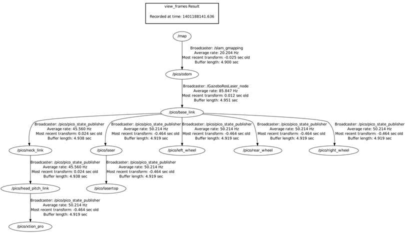
Exploration
Explore_stage
An existing package which works as a goal planner, SLAM and navigation stack, is the explore_stage package. This package is an algorithm that interacts with GMapping to create a map to find exits and tries to navigate by launching a node in Move_base. Which is useful in maze solving case. In order to start this package, again a launch file is made. The same local and global costmap settings have been used as in the previous packages.
The following problems occur: when using RVIZ, it can be seen that a path is planned to an exit, but most of the time the pico seems stuck. Also, when defining a new goal manually by RVIZ, it repeats saying that a node is added on the coordinates: X.X and X.X but the pico does nothing. It also repeats the following warning: Entropy has not been updated. Loop closure opportunities may be ignored.
Within the given time limit, it was not possible to make the Explore_stage package work as desired. The choice is made to continue with GMapping and Move_base in addition with a goal_planner and arrow recognition created from scratch.
Goal planning - OpenCV
The goal planner makes use of different messages and data types. The most important messages and data types which form the basis of the goal planner algorithm are given below.
| Datatype | Purpose |
|---|---|
| Odometry | Odometry data from pico |
| OccupancyGrid | Map data generated by Gmapping stored in a vector |
| MapMetaData | Map information such as resolution and position of origin |
| LaserScan | Laser data |
| MoveBaseActionFeedback | Position and orientation from Pico |
| MoveBaseAction | Allows publishing a goal to move_base |
Strategy
The strategy of the goal planner is chosen to be frontier based. The idea is that the destination goals of the pico are set around the lines between known and unknown area. This can be seen as an explorer which tells pico to explore all unknown areas. This is done with OpenCV by subscribing on the /Map topic on which a matrix/image of a map is published by GMapping. With some tools of the OpenCV library, this image of a map is processed in order to publish Cartesian coordinates to Move_base as a goal. Since, GMapping updates the map in time, new goals are set every time a map is updated. When multiple goals are given, the closest goal to pico is chosen as the primary goal. The choice of the correct primary goal will change when an arrow is detected. This will be explained in the next paragraph.
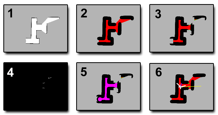
To retrieve goals from the map data the following steps are implemented:
1: The laser data is converted to an image which can be processed using OpenCV. The laser data is provided as a vector in which the walls have a value of 100, the known area have a value of 1 and the unknown area have a value of 0. In the generated picture the walls are colored black, the known area white and the unknown area grey.
2: All black pixels are inflated using a circle of a certain radius depending on the inflation radius chosen in the move_base. The color of the (remaining) known area is changed to red.
3: All pixels of the unknown area (gray) which neighbor known area (red) are inflated by a square. This inflation is implemented to filter noise and remove areas which are unreachable. Next, all boundaries between known and unknown area are colored green.
4: A binary is created for the green pixels only. This binary input is used to detect lines. The line detection is done by a hough line transform. The midpoint of each line will be set a provisional goal.
5: Each goal will be evaluated for reachability. To check this, a floodfill (pink) with Pico as starting point is used. The entry of the maze is closed with an ellipse so no goals will be found at the entry of the maze. All goals lying in the floodfilled area are considered as valid goal targets. Goals which do not lie in the flooded area are discarded.
6: At this point multiple valid goals are available but only one goal can be used as a goal to drive to. First the closest goal in front of pico is given priority. If there are no valid goals in front of pico, the closest goal behind pico will be chosen.
The image below shows the map processing for goal planning in several steps.
During the developing of the goal planner several issues occurred and are solved.
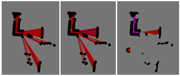
An issue occurs when there are a few laser beams passing through a hole in the wall or just around a corner. It is possible that a goal is set at the frontier of these few laser beams. Since it is not possible for pico to reach these goals, pico will go to its recovery mode. To solve this problem, a floodfill algorithm is used. Unknown area will be inflated and the area starting from pico will be floodfilled. The remaining area is seen as the known area. This way, unreachable areas will be filtered. This can be seen in the pictures given below. The pink area in the right figure is the floodfilled area.
Another issue is the area behind pico at start, which will be seen as a frontier. It is therefore possible that the goal planner sets its goal to the start and tries to reach the unknown area. This problem is solved by adding an arc behind the starting position of pico in the OpenCV images which closes the entrance. Therefore no goal will be set at this position.
Also an issue occurs when there is a frontier near a wall which is not detected by the laser data yet. The goal will be set near this the wall and the pico will not be able to reach this goal, as it is inside the inflated area as soon as pico has detected the wall. This problem is solved by inflating the unknown area. The goal will be set with an offset from the frontier. This problem was also solved by the fact that GMapping updates its map. The pico will see the wall when it moves towards the goal and a new goal will be set. However, if it takes too much time to update the map and process the data, this map updating would not solve the problem.
Recovery mode
If no valid goals are found, no path can be planned to a goal. Therefore pico will not move and no new goals will be planned. In this situation pico is stuck and a recovery is needed. If pico does not move for a certain time, the recovery mode will be initialized. First it is checked depending on the laser data if pico can move forward. If this is not possible Pico will rotate at his current position. Moving forward or rotating causes gmapping to update the map. From the updated map new valid goals can be found.
Initialization
At the startup, the goal planner does not recieve enough information to plan a valid goal point. Information such as the map and pico's orientation are not received yet. In order to get all the necessary data, pico first needs to move. Therefore an initialization is integrated. In this integration pico will move forward for 0.5m. By moving forward all the necessary information will be received by the goal planner and the normal algorithm as described above will provide pico with new goal points.
Arrow recognition - OpenCV
Strategy
The arrow detection node will publish alongside the goal planner node. The idea is to process the image of the camera in the following way: the image of the camera is converted from red-green-blue (RGB) to hue-saturation-value (HSV) (picture 1). A double for-loop is used to convert every red-tinted pixel to black. A binary (two-colour) image is created based on the black and non-black colours (picture 2). This image is then blurred and an edge detection algorithm gives an output of the edges that it can find (picture 3).

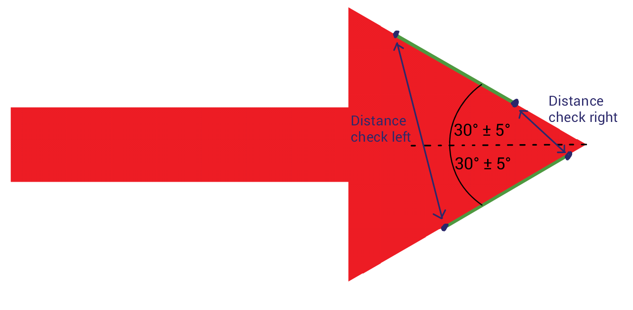
The list of edges is the basis for the arrow recognition, all lines are defined from left to right (so: x1 < x2). Lines are defined as follows: Vec4i line[x1,y1,x2,y2]. The lines are filtered, and the ones that remain are lines with a slope of +/-30 with a +/- 5 degrees margin. All lines with a negative slope are compared with all lines that have a positive slope. Both the +30 [deg] and the -30 [deg] line have a beginning and end point. If the left (begin) points are close enough to each other (3 pixels), the output is "LEFT ARROW", and vice versa. The arrow detection node publishes 0 when no arrow is found and -1 and 1 for the left and right arrow respectively.
The image below shows the +/-30 [deg] lines which this algorithm focuses on:
Integration
An integration plan is necessary for the nodes to communicate properly and produce meaningful results. The following nodes needed to be linked:
- GMapping;
- Move_base;
- Arrow recognition;
- Goal planner.
Using rqt_graph, the following graph is given:

The picture above describes the nodes that are communicating and the topics that they use. Both Move_base and GMapping already incorporate important aspects such as the laserdata and internal communication. Both the goal planner and arrow recognition script are self made and needed manual integration of the following aspects:
- Retrieve map data in goal planner;
- Retrieve image data in the arrow recognition;
- Send the arrow direction to the goal planner;
- Retrieve arrow direction in the goal planner;
- Combine possible goal locations with arrow input and send a simple goal to Move_base;
- When there are no goals, send a recovery goal to refresh the map and find new pathways.
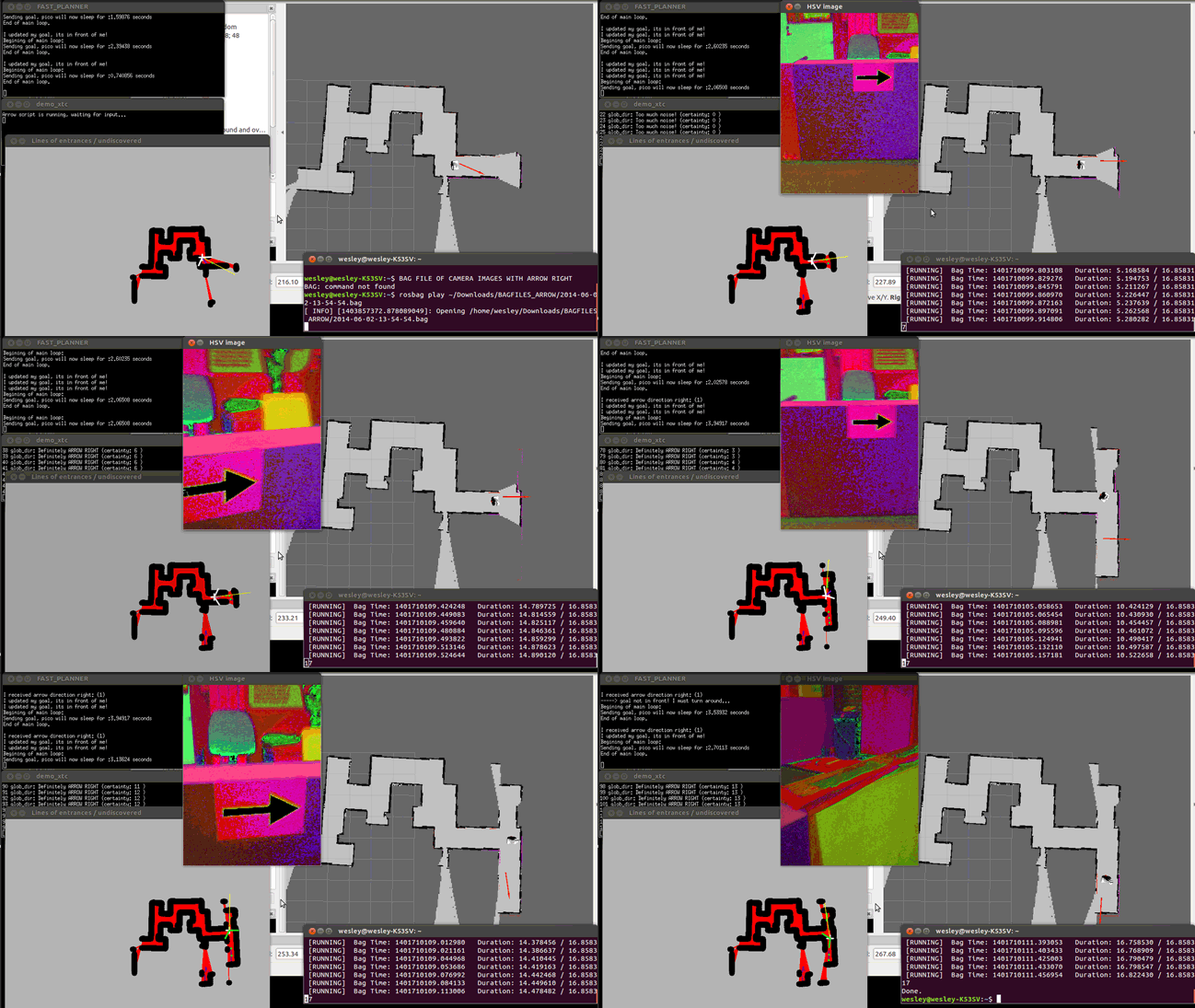
Two of the big challenges in the goal planner are the conversion of the map to a useful image and the decision making in case of arrow input. The animated picture below shows the simulation where Pico is given the "arrow right" input by playing a bag file on the background. This is where Pico is forced to make a decision.
Explanation of the picture:
- White cross = location of Pico;
- Purple line = looking direction of Pico;
- Other white lines from Pico's location = Pico's field of view (Goals in front have high priotity);
- Green lines from Pico's location = Pico's field of view with arrow input (Goals to the right or left have high priority);
- Yellow line = The direction Pico would choose without arrow input.
The picture clearly shows that Pico is ignoring the goals that it would otherwise head for. Pico is choosing the direction that the arrow is pointing towards.
Results
| Corridor challenge: | Simulation 1: |
|---|---|
 |
 |
| Simulation 2: | Maze challenge: |
|---|---|
 |
 |
Evaluation
The maze competition was passed within 2 minutes and 40 seconds. As seen in the video of the maze competition, Pico had problems passing the second crossing with two dead ends. This has cost us a lot of time, but Pico was able to unstuck itself thanks to its built-in recovery mode.
Previous practical tests have shown that Pico can find any exit in a much shorter timespan. At the moment it is not certain what exactly went wrong. A potential cause could be a flaw in the goal planner node which slows down the script. Another problem during the competition was that the GMapping script was consuming an unusually high amount of processor power.
For the maze competition with a relative simple structure (straight corridors, perpendicular corners and easy to detect deadends), our approach was at disadvantage because of complexity. A properly working case-detector could have been faster. Our solution would have a big advantage in a complex maze, with non-rectangular shapes and narrow passings included. Pico would be able to plan goals and move towards them in order to explore the whole area and eventually solve the maze.
The disadvantages of the chosen solution:
- A time consuming (inefficient) goal planner script;
- A complex solution for a relatively simple challenge.
The advantages:
- Reliability, the robot will only stop if everything is explored and remaining goals are unreachable;
- Can solve any maze, strange shapes or too narrow pathways don't influence the resolvability;
- Can recognise dead ends and moves on to look for alternatives.
Practical issues
TF tree
Viewing a tf tree can be done by:
$ rosrun tf view_frames
GMapping and Move_base in simulations
1. Start Gazebo:
$ gazebo
2. Using another terminal, spawn the maze:
$ rosrun gazebo_map_spawner spawn_maze
3. Launch PICO:
$ roslaunch pico_gazebo pico.launch
4. Start RViz to visualize how PICO perceives the world through its sensors.
$ rosrun pico_visualization rviz
5. Launch the gmapping plugin for PICO
$ roslaunch pico_2ndnav gmap.launch
6. Launch the move_base package for PICO to navigate through the maze with the preferred settings.
$ roslaunch pico_2ndnav move_base.launch
Explore_stage in simulations
1. Get in the right directory:
$ roscd explore_stage
2. Launch the explore_stage launch file:
$ roslaunch explore_slam.launch
Goal planning - OpenCV
In some cases, your script will not find the required include:
#include <move_base_msgs/MoveBaseActionFeedback.h> // Contains the location of pico
The solution (ubuntu command):
sudo cp -a /opt/ros/groovy/stacks/navigation/move_base_msgs/msg_gen/cpp/include/. /opt/ros/groovy/include/
The OpenCV C++ files can be compiled using one of the given commands below. For the g++ command, the packages need to be specified manually.
$ g++ demo_opencv.cpp `pkg-config opencv --cflags --libs` -o demo_opencv
Or you can make have ROS find the libaries for you:
$ rosmake demo_opencv
Executing the program:
$ ./demo_opencv <argcount> <arg(s)>
Goal planning - OpenCV Troubleshooting
There have been problems with the OpenCV and Highgui libraries (static libraries). This problem can be solved by replacing the following code:
// #include "cv.h" // (commented out)
#include "opencv2/opencv.hpp"
// #include <highgui.h> // (commented out)
#include <opencv/highgui.h>
The program might not always respond to input, this is can be due to a subscription to the wrong topic. Make sure you are streaming the images and check the ros-topic with:
rostopic list
Then the output gives "/pico/camera", "/pico/asusxtion/rgb/image_color", or a different name. Replace the referece in the following line of code:
ros::Subscriber cam_img_sub = nh.subscribe("/pico/asusxtion/rgb/image_color", 1, &imageCallback);
Runnig OpenCV on an image stream from a bag file:
In three separate terminals:
roscore
rosbag play <location of bag file>
./demo_opencv
Arrow recognition
The image is cropped using:
cv::Rect myROI(120,220,400,200);  // Rect_(x,y,width,height)
cv::Mat croppedRef(img_rgb, myROI); // The window is 480 rows and 640 cols
Pico experiment setup
Terminal 1:
ssh pico
pico123
pstart
Terminal 2:
pico-core
rviz rviz
Terminal 3:
ssh pico
pico123

roscd gmapping
**check if group 11 has gmapping if so delete gmapping map**
cd ..
rm -rf gmapping

cd ros/groovy/emc/groups/emc07
svn up

roscd pico_2ndnav
roslaunch pico_2ndnav gmap.launch
Terminal 4:
ssh pico
pico123
roscd pico_2ndnav
roslaunch pico_2ndnav move_base.launch
Terminal 5:
ssh pico
pico123
roscd goal_planner_roel2
rosmake goal_planner_roel2
./bin/goal_xtc
Terminal 6:
ssh pico
pico123
roscd demo_opencv_wesley
rosmake demo_opencv_wesley
./bin/demo_xtc
Time Table
| Lectures | Group meetings | Mastering ROS and C++ | Preparing midterm assignment | Preparing final assignment | Wiki progress report | Other activities | |
|---|---|---|---|---|---|---|---|
| Week 1 | |||||||
| Pim | 2 | ||||||
| Roel | 2 | ||||||
| Maurice | 2 | ||||||
| Wesley | 2 | ||||||
| Glenn | 2 | ||||||
| Week 2 | |||||||
| Pim | 2 | 2 | 4 | 3 | |||
| Roel | 0 | 2 | 10 | 6 | |||
| Maurice | 2 | 2 | 6 | 3 | |||
| Wesley | 2 | 2 | 4 | 2 | |||
| Glenn | 2 | 2 | 5 | 2 | |||
| Week 3 | |||||||
| Pim | 2 | 1 | 12 | 2 | |||
| Roel | 2 | 4 | 10 | 2 | |||
| Maurice | 2 | 3 | 10 | 4 | |||
| Wesley | 2 | 3 | 10 | 1 | |||
| Glenn | 2 | 2 | 13 | 4 | |||
| Week 4 | |||||||
| Pim | 2 | 5 | 1 | 7 | 3 | ||
| Roel | 2 | 5 | |||||
| Maurice | 2 | 5 | 15 | ||||
| Wesley | 2 | 5 | 9 | 1 | |||
| Glenn | 2 | 5 | 6 | 1 | |||
| Week 5 | |||||||
| Pim | 2 | 2.5 | 7 | 0.5 | |||
| Roel | 2 | 2.5 | 6 | 1 | |||
| Maurice | 2 | 2.5 | 8 | 0.5 | |||
| Wesley | 2 | 5 | 7 | 3 | |||
| Glenn | 2 | 2.5 | 7 | ||||
| Week 6 | |||||||
| Pim | 4 | 6 | |||||
| Roel | 4 | 6 | |||||
| Maurice | 4 | 8 | |||||
| Wesley | 4 | 8 | 14 | ||||
| Glenn | 4 | 8 | 1 | ||||
| Week 7 | |||||||
| Pim | 2 | 2.5 | 10 | ||||
| Roel | 2 | 4 | 8 | 3 | |||
| Maurice | 2 | 4 | 9 | 2 | |||
| Wesley | 2 | 4 | 2 | 12 | |||
| Glenn | 2 | 2 | 8 | 5 | |||
| Week 8+9 | |||||||
| Pim | 4 | 1.5 | 23 | ||||
| Roel | 2.5 | 20 | 4 | ||||
| Maurice | 0.5 | 20 | 2 | 4 | |||
| Wesley | 0.5 | 29 | |||||
| Glenn | 10 | 5 | |||||
