Mobile Robot Control 2023 Group 5: Difference between revisions
Tag: 2017 source edit |
Tag: 2017 source edit |
||
| (2 intermediate revisions by the same user not shown) | |||
| Line 15: | Line 15: | ||
==Introduction Assignment 0== | ==Introduction Assignment 0== | ||
*'''Video of the robot's performance in real life''' | *'''Video of the robot's performance in real life''' | ||
https://tuenl-my.sharepoint.com/:v:/g/personal/r_li1_student_tue_nl/EQCPnYnKB8tOnGPgaSa9pbsBrzGMamXEKJRJ3B8zLKiMyg?e=fiKc62 | https://tuenl-my.sharepoint.com/:v:/g/personal/r_li1_student_tue_nl/EQCPnYnKB8tOnGPgaSa9pbsBrzGMamXEKJRJ3B8zLKiMyg?e=fiKc62 | ||
==Navigation Assignment 1== | ==Navigation Assignment 1== | ||
| Line 59: | Line 54: | ||
*'''Observe the Behaviour in Simulation''' | *'''Observe the Behaviour in Simulation''' | ||
# | #We detect both the matrix one and real one to compare the accuracy; Inaccurate part: we cannot drive the car back the exact start point. There’s and error from 3-10cm on both x and y axis. | ||
#The effect of using certain_odom is much better than using uncertain_odom. | |||
#If use uncertain odometry, the odometry frame would be different from the robot frame, which means the output odometry would not as predicted since they are measured in different corordinate. And the uncertain one has much larger error caused by noise that increased by time. | #If use uncertain odometry, the odometry frame would be different from the robot frame, which means the output odometry would not as predicted since they are measured in different corordinate. And the uncertain one has much larger error caused by noise that increased by time. | ||
#For the final challenge we need to serve the tables, which means the robot has to move around the ‘room’, cosing relatively long time. With time increasing, so as the distance increasing, the error and noise in the odometry information would be also increasing, Thus, ode info would be more and more unreliable, which lead to the main reason we dont want t use it | #For the final challenge we need to serve the tables, which means the robot has to move around the ‘room’, cosing relatively long time. With time increasing, so as the distance increasing, the error and noise in the odometry information would be also increasing, Thus, ode info would be more and more unreliable, which lead to the main reason we dont want t use it | ||
| Line 70: | Line 66: | ||
https://tuenl-my.sharepoint.com/:v:/g/personal/r_li1_student_tue_nl/EdQRN6zom2NGuyOyk_MPzrMBwy9nmzLAt2u_WNmP7ZDEvQ?e=RZSAYA | https://tuenl-my.sharepoint.com/:v:/g/personal/r_li1_student_tue_nl/EdQRN6zom2NGuyOyk_MPzrMBwy9nmzLAt2u_WNmP7ZDEvQ?e=RZSAYA | ||
In reality, maybe due to increased noise and vehicle slippage, the localization information became more inaccurate. | |||
==Localisation Assignment 2== | ==Localisation Assignment 2== | ||
Latest revision as of 00:01, 8 July 2023
Group members:
| Name | student ID |
|---|---|
| Yuzhou Nie | 1863428 |
| Ronghui Li | 1707183 |
| Guglielmo Morselli | 1959301 |
Introduction Assignment 0
- Video of the robot's performance in real life
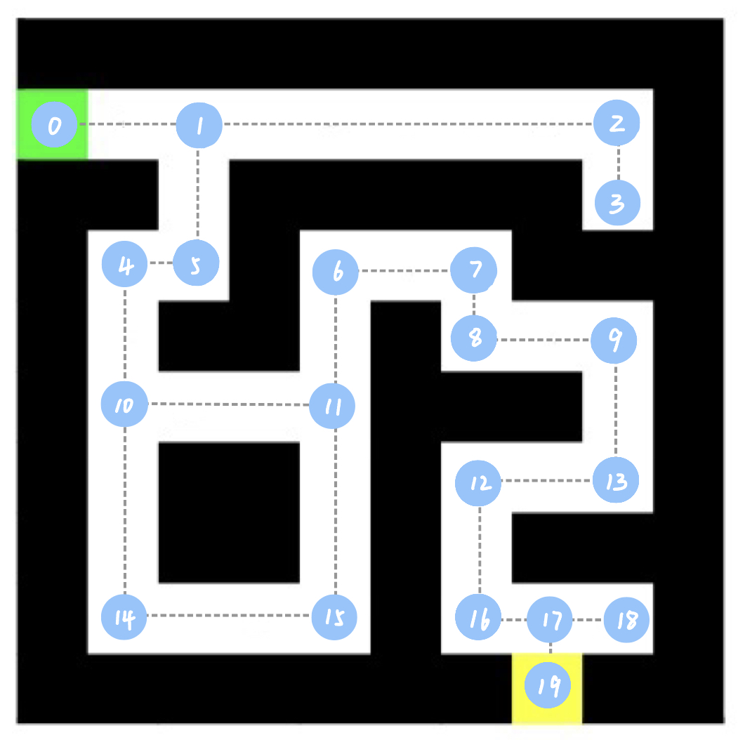
- How could finding the shortest path through the maze using the A* algorithm be made more efficient by placing the nodes differently?Sketch the small maze with the proposed nodes and the connections between them.Why would this be more efficient?
By placing nodes at key points(junctions for example) could reduce the total number of nodes and simplify the graph, which lead to a less computational effort.
(add picture)
- Description of the main idea
We choose to implement the Artificial Potential Field (APF) algorithm for obstacle avoidance in robot navigation. It uses laser scanner data to detect obstacles, calculates repulsive forces based on obstacle proximity, converts these forces into velocity commands, and sends these commands to the robot, enabling dynamic navigation.
- Screen recordings of the simulation results
- Video of the robot's performance in real life
Localisation Assignment 1
- Keep Track of our location
The program successfully reports the information in the odometry message of current time step and the difference between the previously received odometry message and the current message.
- Observe the Behaviour in Simulation
- We detect both the matrix one and real one to compare the accuracy; Inaccurate part: we cannot drive the car back the exact start point. There’s and error from 3-10cm on both x and y axis.
- The effect of using certain_odom is much better than using uncertain_odom.
- If use uncertain odometry, the odometry frame would be different from the robot frame, which means the output odometry would not as predicted since they are measured in different corordinate. And the uncertain one has much larger error caused by noise that increased by time.
- For the final challenge we need to serve the tables, which means the robot has to move around the ‘room’, cosing relatively long time. With time increasing, so as the distance increasing, the error and noise in the odometry information would be also increasing, Thus, ode info would be more and more unreliable, which lead to the main reason we dont want t use it
- Observe the Behaviour in Reality
Here attached the video of coco's performance in real life:
In reality, maybe due to increased noise and vehicle slippage, the localization information became more inaccurate.
Localisation Assignment 2
- Explore the code-base
- The 'PracticalFilter' class is inheritances from 'PracticalFilterBase'. The 'PracticalFilterBase' provided basic function for a generic particle filter, and 'PracticalFilter' extends the function by implementing additional methods.
- The 'ParticleFilter' relies on the 'Particle' for its operations.
- The 'PracticalFilterBase::propagateSamples' method in the 'PracticalFilter' class is responsible for applying the propagation to all particles, and the 'Practical::propagateSample' method in the 'Practical' class is responsible for the propagation of individual particles.
- Initialize the Particle Filter
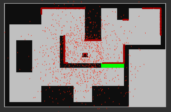
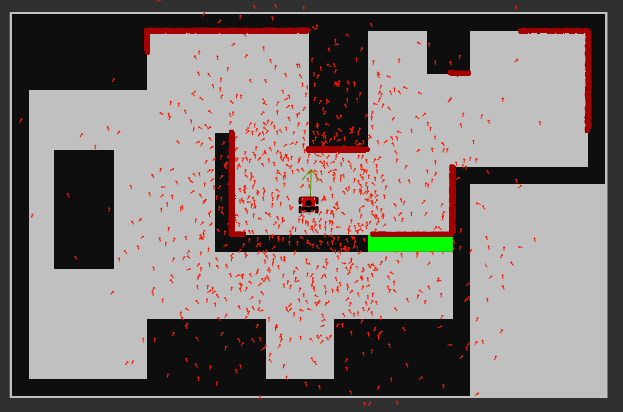
The particle filter begins with a set of particles randomly distributed throughout the robot's known map or environment. Each particle represents a potential state of the robot, including its position and orientation, and the particle cloud can be initiliazed either through a uniform or a normal distribution. As the following figure shows, particles with Gaussian noise and random initial poses are constructed along with their filters. There are 1000 particles being generated and the center of them is the initial position of the robot.
- Calculate the filter prediction
After generated the particle filters, now the prediction of the filter (average pose) should be calculated. The average pose can be obtained by iterating through the particle set while performing accumulation calculations on the position. The green arrow in the figure below shows the visualization of the average pose of particles generated around the initial point of the robot.
- Propagation of Particles
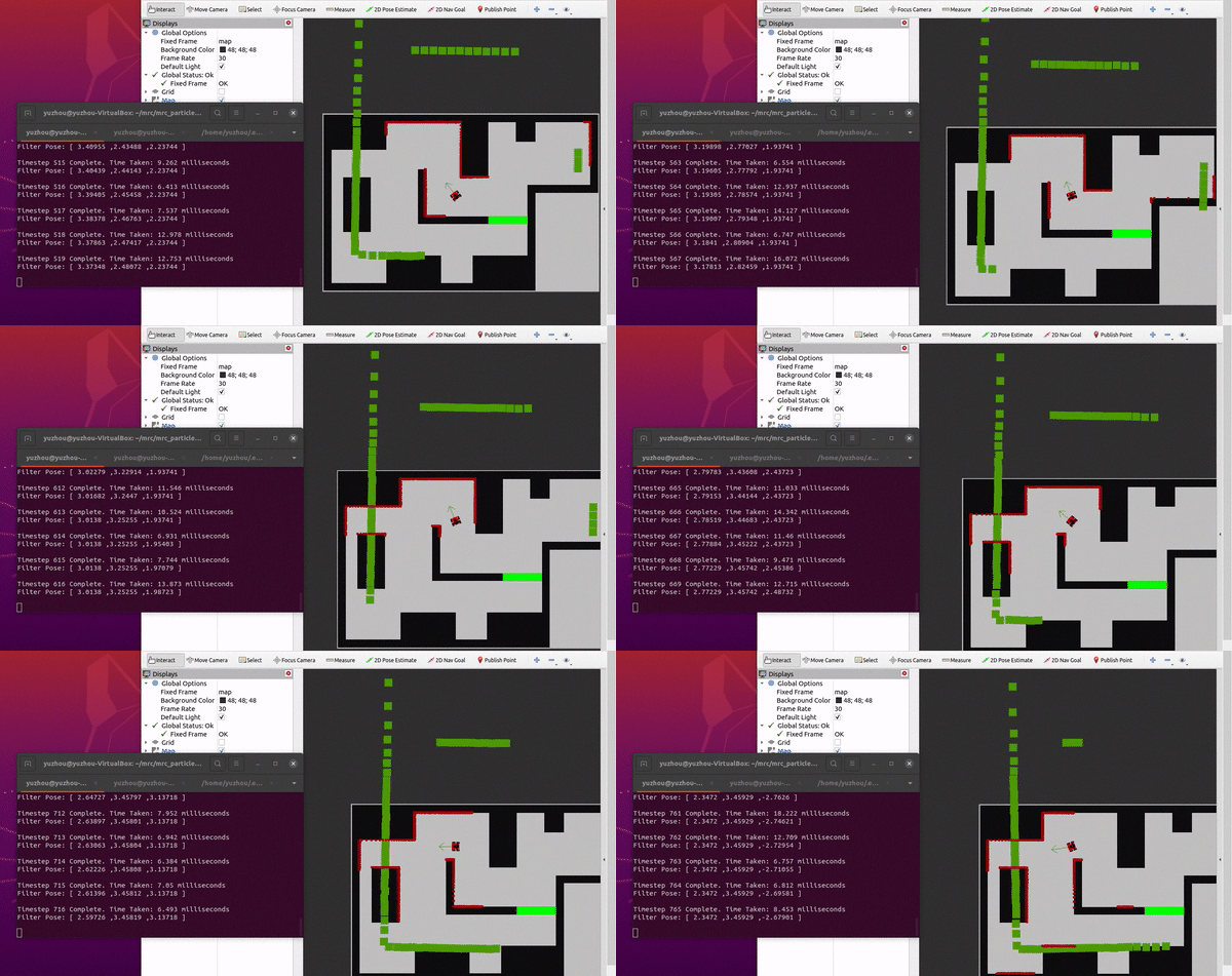
The robot would move around instead of staying still. Thus, updating the positions and orientations of particles based on the robot's motion model is crucial. In this step, each particle undergoes translation and rotation according to the robot's motion information while accounting for the noise and uncertainties in the motion model. The simulation result is shown as the gif below. With the propagation of particles, now the pose prediction (average pose) can be generated even though the robot is moving, getting the primary localization information.
- Computation of the likelihood of a Particle
Calculating the likelihood of a particle is an important step for particle filter. It is used to determine the weight of each particle, which in turn affects the sampling probability in the subsequent resampling step. By calculating the likelihood of a particle, the particle filter can better estimate the true state of the robot and assign more weight to particles that have a higher match with the observed data.
Generally there're two sub-steps to accomplish this step. First, generate the prediction of the expected measurements (ranges to obstacles) based on laser. Then, compute the likelihood of each measurement relative to this prediction using the parameters set in the config file (incorporating noise).
- Resampling our Particles
Now the particle filter method is almost done. But the resampling of particles is also crucial for the optimization of performance. Multinomial method was chosen as the resampling method. This multinomial resampling method samples particles based on their weights and in a probabilistical way, such that particles with higher weights have a greater probability of being selected into the new particle set, while particles with lower weights have a smaller probability of being selected. This allows the particle set to better reflect the posterior probability distribution, thereby improving the performance of the filter.
- Performance and analysis
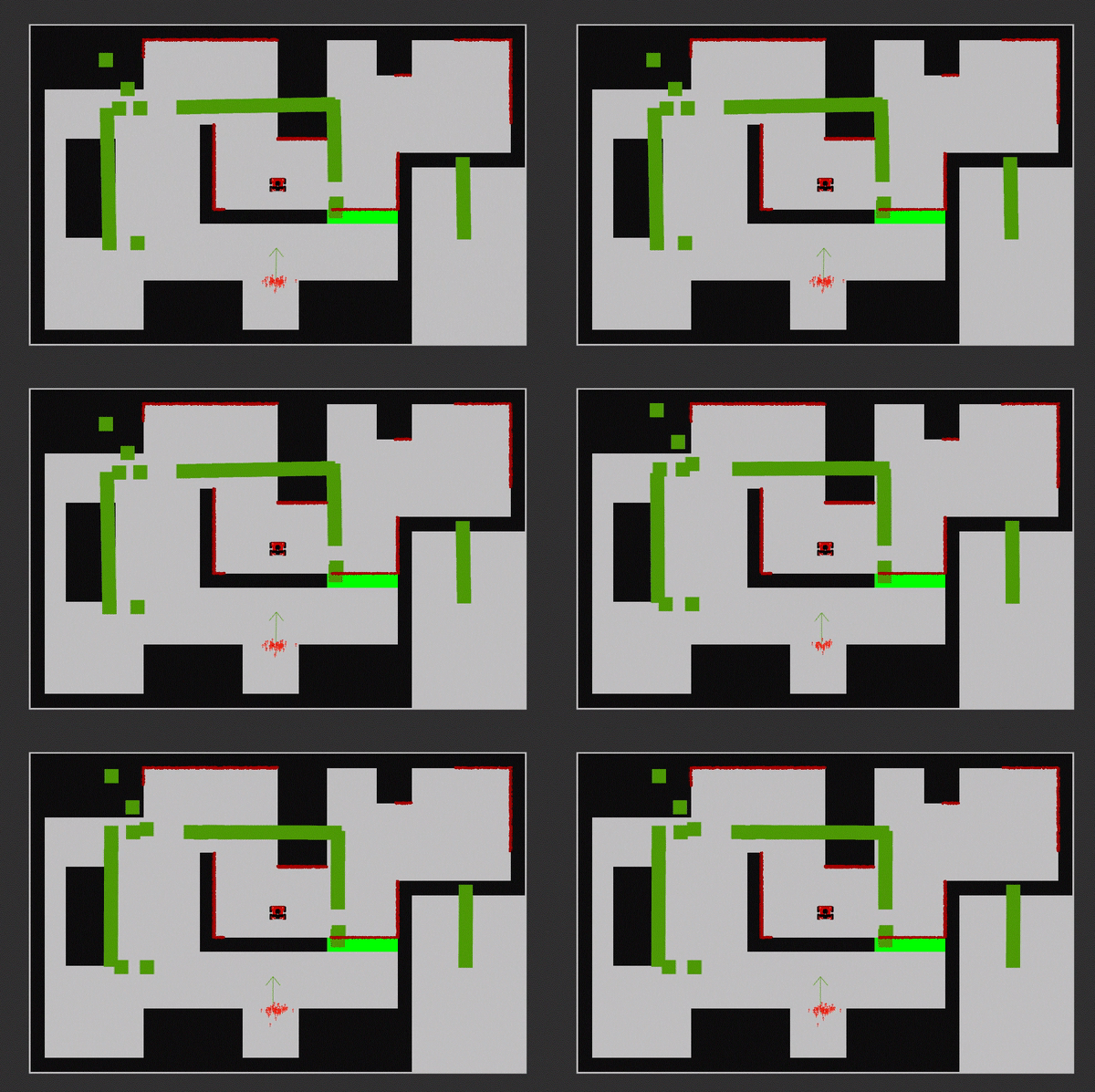
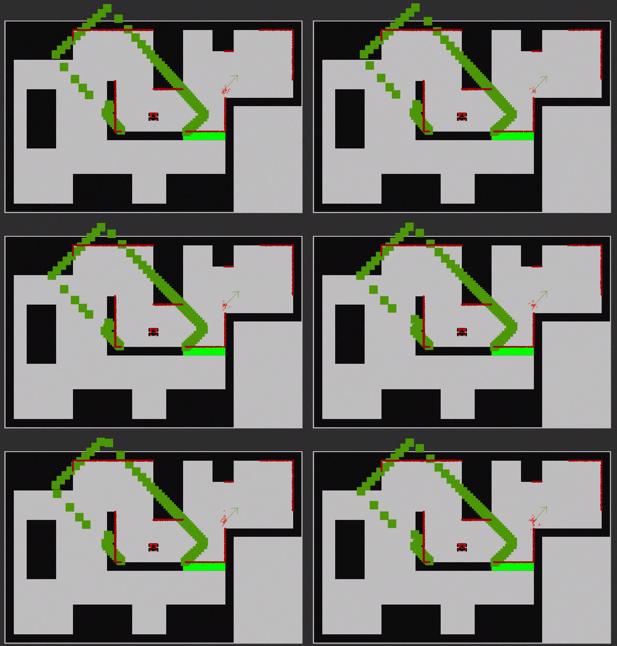
After all the steps above, the particle filter method should be achieved. Thus, now the RVIZ and mrc-teleop can be utilized to simulate the performance of this method for localization. The simulation result is as the below gifs shows. As shown in these two images, the likelihood and resample operations of the particles are working well. However, the only problem is the laser prediction (the green blocks) that similar to the figure shown in step 3), they are not accurate for not matching with the structure of the map. This results significant interference with the overall pose estimation of the particles. Despite continuously debugging the code and checking the map creation and loading,the root cause of the problem hasn't been spotted. Therefore, it is possible that there is an issue with the simulator system, which prevents the sensors from clearly detecting the boundaries created in the map.
