Mobile Robot Control 2023 Ultron: Difference between revisions
| (65 intermediate revisions by 4 users not shown) | |||
| Line 47: | Line 47: | ||
The first step in tackling the Restaurant Challenge was to build the requirements based on the system specifications. This entailed carefully considering the robot and the environment in which it was used, as well as the overarching stakeholder requirements of safety, time, and customer intimation. We were able to develop a set of requirements that would guide our efforts toward successfully completing the challenge by taking these factors into consideration. | The first step in tackling the Restaurant Challenge was to build the requirements based on the system specifications. This entailed carefully considering the robot and the environment in which it was used, as well as the overarching stakeholder requirements of safety, time, and customer intimation. We were able to develop a set of requirements that would guide our efforts toward successfully completing the challenge by taking these factors into consideration. | ||
== | ==Approach== | ||
===Requirements=== | ===Requirements=== | ||
[[File:Requirementsframe.jpg|thumb|Functional Requirements]][[File:Requirementsframe2.jpg|thumb|Non functional requirements]] | [[File:Requirementsframe.jpg|thumb|Functional Requirements]][[File:Requirementsframe2.jpg|thumb|Non functional requirements]] | ||
Requirements are a crucial part of the design process as they define the goals and constraints of a project. By establishing clear requirements, a team can ensure that their efforts are focused on achieving the desired outcome and that all necessary considerations are taken into account. In the case of the Restaurant Challenge, we took the system setting from the previous paragraph as well as challenge into account when designing the specifications for our requirements. This allowed us to develop a set of requirements that were tailored to the specific needs of the challenge, | Requirements are a crucial part of the design process as they define the goals and constraints of a project. By establishing clear requirements, a team can ensure that their efforts are focused on achieving the desired outcome and that all necessary considerations are taken into account. In the case of the Restaurant Challenge, we took the system setting from the previous paragraph as well as challenge into account when designing the specifications for our requirements. This allowed us to develop a set of requirements that were tailored to the specific needs of the challenge. This allowed us to clearly define the capabilities and constraints of the robot, as well as the overarching goals of the challenge. | ||
Our requirements included the ability for the robot to deliver food and drinks, detect dynamic and static obstacles, navigate autonomously using its sensors and a defined map in real-time, communicate with humans to avoid blocking, and avoid static and dynamic obstacles. The robot was also equipped with a lidar sensor and a source of energy. | |||
Our | Our requirements were divided into three groups: obstacle detection, safety, and reliability. For obstacle detection, the obstacles should be classified into dynamic and static obstacles. We specified that for every static object/obstacle detected within 0.7m range of the robot, it should plan a local path such that it avoids the obstacle and move along that local path. For every dynamic obstacle detected within the 0.7m range of the robot, the robot should send an audio command asking to move the dynamic obstacle away from the path, wait for some time until the object is moved and continue along the path. If the dynamic obstacle does not move within a certain amount of time, the robot should compute a local path to avoid the obstacle and move along that path. We did not specify the exact time to wait as it was an early process, and we could not estimate or know the exact computation overload. | ||
For safety, we specified that the maximum speed of the robot should be undefined for the same reason, and that the minimum distance to static and dynamic obstacles should be different. The frequency of the lidar sensor should be updated at least at a certain frequency, such that it is sufficient to capture both static and dynamic obstacles. | For safety, we specified that the maximum speed of the robot should be undefined for the same reason, and that the minimum distance to static and dynamic obstacles should be different. The frequency of the lidar sensor should be updated at least at a certain frequency, such that it is sufficient to capture both static and dynamic obstacles. | ||
| Line 64: | Line 62: | ||
For reliability, we specified that global and local path planners should be restricted by time constraints. The maximum delivery time should not exceed 10 minutes as this was given to us as an overall constraint. | For reliability, we specified that global and local path planners should be restricted by time constraints. The maximum delivery time should not exceed 10 minutes as this was given to us as an overall constraint. | ||
By | By specifying our requirements, we were able to clearly define the capabilities and constraints of the robot, ensuring that our efforts were directed towards achieving success in the challenge. | ||
[[File:DataFlowDiagram.jpg|thumb|Data Flow Diagram]] | [[File:DataFlowDiagram.jpg|thumb|Data Flow Diagram]] | ||
| Line 71: | Line 69: | ||
The diagram for data flow was created based on the available data to the robot from its environment through its sensors namely, the bumper data, laser data and the odometry data, as well as the known data from the map and the input table sequence. Each of these inputs were used in different segments of the code to generate intermediate data. The odometry and laser data were used to perform localization which in turn gives the pose (position and orientation) of the robot. The laser data was also used in the process of detecting obstacles and doors. This data is used further down the line in other processes like local and global path planning. Overall, the smooth transfer and interaction of data between each individual part of the code ensures that the robot moves in a predictable manner.[[File:StateFlowDiagram1.jpg|thumb|State Diagram|border]] | The diagram for data flow was created based on the available data to the robot from its environment through its sensors namely, the bumper data, laser data and the odometry data, as well as the known data from the map and the input table sequence. Each of these inputs were used in different segments of the code to generate intermediate data. The odometry and laser data were used to perform localization which in turn gives the pose (position and orientation) of the robot. The laser data was also used in the process of detecting obstacles and doors. This data is used further down the line in other processes like local and global path planning. Overall, the smooth transfer and interaction of data between each individual part of the code ensures that the robot moves in a predictable manner.[[File:StateFlowDiagram1.jpg|thumb|State Diagram|border]] | ||
===State Diagram=== | ===State Diagram=== | ||
The state diagram describes how the code was split into segments. | The state diagram describes how the code was to be split into segments. Firstly, the robot has to find its initial position using localization techniques as soon as the robot is turned on. Using the input form the user, we compute the global path which gives you the list of grids that must be traversed to reach a particular table. Once the path is established the local path planner takes in the list of grids one by one and performs local navigation. The local path planning ensures that the navigation between two grids is collision free. | ||
If the path is blocked, we check whether is a door, a static or dynamic obstacle. In case it encounters a door or dynamic obstacle, the robot will request path access. If the local path planner is unable to find a clear path after certain waiting time, the map is updated and a different global path is found, which is then sent to the local navigator to reach the next table. If the table has been reached, the robot will orient itself towards it before announcing its arrival. From here the global path planning takes over to find the path to the next table and the process repeats till the final table is reached. However, the state diagram shown in the figure had many flaws, as were pointed out to us at the mid-term presentation. The major one of which is the breaking of the loop at the Emergency stop state. For the final challenge, however, some of these states were deemed redundant and not a priority for adding into the code. | |||
==Implementation== | |||
First and foremost, it becomes imperative to provide the robot with some information about the environment in which it is to operate. This is achieved by taking the map inputs that can be as accurate to the real world as possible and discretizing them into occupancy grids. Using these occupancy grids, the robot navigates through the restaurant. The grids act as nodes in the A* algorithm and provide information about the occupancy status. | |||
====Map Creation==== | |||
[[File:Grids around table.jpg|thumb|Grids associated with each table]] | |||
The need to automate reading the map data from a json file arose from wanting to create grids for the global path planning for navigation. The json file provided to the team contained the exact location in terms of x and y coordinates for each vertex of the tables and walls in the map and their corresponding vertex numbers (from here on referred to as nodes). The objects "tables", "walls", "doors" and "start area" also contained the connections between the nodes corresponding to their four corners. It was clear from the file that the total size of the restaurant was a 7m by 4.5m almost rectangular space as shown in the figure. At first, a "world" object was hardcoded into the json file that represents the outermost boundary of the map. Each of the objects were read from the json file and stored in different vectors. | |||
[[File:GridmapUlt.png|alt=Grid length bigger than the final grid length used.|thumb|Grid Map with grid size of 0.025m for visualizing]] | |||
To ensure that the reachable grids are safe, the tables and the inner walls were blown up by 0.2m in all directions. The map was then discretized into grids of length 0.025m. All the grids that are inside the blown-up map objects, were made inaccessible to the global path planning. The remaining grid space was deemed open. | |||
The occupancy grids contained in the door region, is marked by the "doorflag", which is true when the grid is inside the door region. Another member variable of the grid called "logodd" gives the likelihood of the grid being occupied. | |||
Each grid possesses a variable that gives list of grids that are connected to it and are present in the open grid list. | |||
A list of grids surrounding a table were chosen and linked to that specific table. These grids are the possible positions the robot can occupy to serve the table and were considered as the end goals for the global path planner. | |||
All of these are utilized to execute the navigation of the robot. | |||
===Navigation=== | ===Navigation=== | ||
The navigation process for mobile robots is categorized into four parts: environmental mapping, path planning, | The navigation process for mobile robots is categorized into four parts: global path planning, environmental mapping, obstacle avoidance and motion control. The global path planning determines the shortest route that the robot has to take from the start to the goal grid. As the robot traverses the global path, based on the laser data, the restaurant is mapped iteratively. | ||
The open space approach is used to identify the heading direction of the robot, locally. Simultaneously, the artificial potential field created prevents collision with its surrounding objects, by computing the control inputs that ensures safety and eventually steers the robot to the goal grid. | |||
====Occupancy Grid Mapping==== | |||
[[File:Occmap.png|thumb|Occupancy grid map of the restaurant]] | |||
Initially the object detection was done using the logic that if the laser point hit an object within a scan radius of 0.7m, the corresponding grid was identified and updated as occupied such that local path planner can update it. However, there were few issues. As the grid size was decreased, the grids which fell inside the object and not on the periphery of the object were considered as unoccupied grids, although they were occupied in reality. | |||
To overcome this, we decided to use occupancy grid mapping that represents the occupancy status of a grid based on the laser data, with a score called logodd value for each grid. This value is updated based on the laser hit points and the free space from the ray casting. | |||
The new algorithm works as follows, | |||
*All the grids that connect the current grid of the robot, to the hit point of each ray is computed using Bresenham's algorithm. | |||
*The logodd value for the final hit point grid is increased by +1 while the intermediate grids are decreased by -0.5 | |||
*The logodd value is increased by +0.7 for clouds of grid up to 3 layers, that surround the hit point gird. | |||
*The logodd value can take a maximum of +100 if the grid is occupied and a minimum of -100 if it is free | |||
*Each grid is initialized with a logodd value of 5. | |||
*Based on the final output of the logodd value, the likelihood of an object being present in that space can be computed. This was roughly plotted using the openCV package. | |||
====Global Navigation==== | ====Global Navigation==== | ||
[[File:Rerouting Obstacle.gif|thumb|Path planned using A* and Rerouting]] | |||
The A* algorithm is a widely used path planning algorithm for autonomous robots. Its importance to the challenge comes in the form of finding the shortest path between two points in the map. It calculates the cost to travel to a given grid and plans the path such that this cost is the least. | The A* algorithm is a widely used path planning algorithm for autonomous robots. Its importance to the challenge comes in the form of finding the shortest path between two points in the map. It calculates the cost to travel to a given grid and plans the path such that this cost is the least. | ||
Firstly, based on the current position of the robot, the starting grid ID is obtained. Then closest grid associated to the table received as an input from the user, is determined from this grid. With these grid IDs as start and end IDs, the A* algorithm was implemented. These end IDs were also chosen based on the updated logodd values from the occupancy grid mapping algorithm. | |||
This comes handy when the final goal is inside an object, in which case the A* algorithm is recomputed from the failure point. | |||
The list of grids to reach the goal using the shortest path was found and sent to the open space algorithm. When node that is being sent has a logodd value more than the initialized value, the grids are skipped. If sufficient grids are skipped in the computed path, the path is forfeited and the A* algorithm is called again to calculate an alternate path from that position. After sending the grid ID's one by one the bot would reach that table with help of open space. After reaching that grid the start grid ID is updated to the previously reached ID and the goal is set as one of the grids in the cloud of grids surrounding the next table from the table sequence and then path was again computed. This process repeats until the final table is reached. | |||
In order to obtain good navigation performance and accurate obstacle avoidance, it is necessary to have another type of navigation, namely local navigation that allows the robot to be truly autonomous in decision making in terms of moving to the next goal position. | |||
* | |||
==== | ====Local Navigation: Open space and Artificial potential field(APF) approach==== | ||
* | =====Path following===== | ||
The local path planner receives the list of grids that are to be reached one by one from the A* algorithm. If the grid that is destined is an intermediate grid, the local navigation is adopted until the bot is around a proximity of 0.5m. After reaching within this proximity the open space returns true to show it successfully navigated there. The next grid is then received, and this process is followed until the robot heads to the grid that is associated to the final point of the table. Here, the goal tolerance is set to 0.02m so that the robot reaches the table grid. After this the robot re-orients itself until it faces towards the center of the robot. Once this is achieved, the open space returns true to the A* algorithm to find the path to the next table. | |||
[[File:Obstacle Avoidance Real time.gif|thumb|Obstacle Avoidance]] | |||
=====Obstacle Avoidance===== | =====Obstacle Avoidance===== | ||
======Open space====== | |||
The obstacle avoidance is achieved using the open space approach and the APF. The open space provides an appropriate heading angle by scanning an area within a specific horizon limit, which was set to 0.7m in our trials. The radius of this scan is adaptive and decreases to the distance between the bot and the heading grid position. The heading pose is chosen based on the shortest point on the arc to the heading grid. This pose on the arc along with the scanned arc is sent to the APF to compute the control inputs for the bot. | |||
[[File:Obstacle Avoidance.gif|thumb|Obstacle Avoidance]] | |||
The point on arc is only chosen when the open arc is of sufficient length, i.e. wide enough for the bot to enter. If this is not possible, the robot temporarily marks these grids as blocked and sends false to the A* algorithm to recompute the global path. | |||
Video link to the open space algorithm implemented on the robot in real time - https://tuenl-my.sharepoint.com/:v:/g/personal/a_nadig_student_tue_nl/EZhHaK7-WIZNsT-2XCIXlYkBclsjhFPy8pEfz20meuL0Dw?e=L1xeoy | |||
===== | ======APF====== | ||
The position from the scan arc is received and an attractive potential function is defined using the norm of the distance. For the repulsive field, the closest hitpoint from the laser is obtained and the norm of this distance from the bot is used as the repulsive potential. They are combined together with a thresholding function on the repulsive potential such that it de-activates when the bot is sufficiently far away. | |||
V_attractive = 0.5 ||x - x*||^2, where x denotes the 2D column vector of the robot, x* denotes the heading position received from the open arc. | |||
V_repulsive = 0.5 ||x - x_hit||^2, where x denotes the 2D column vector of the robot, x_hit denotes the closest hit point of the laser. | |||
= | S(x) = kx/(1+kx) - Thresholding function. | ||
==== | Final potential: V = V_attractive / S(V_repulsive); The gradient of this is used as the control input which is converted to robot as linear and angular input based on the holonomic constraints of the bot. <br /> | ||
=====Encountering a door===== | |||
[[File:Door Opening.gif|thumb|Encountering a door]] | |||
If the next grid is inside a door, we check if the door is opened or closed based on the logodd value obtained for the door grids. The door will be closed if the logodd values never decreased. If the logodd value for at least 20 grids inside the door is decreased, then the door is considered open and the loop returns to the open space. If it is declared as closed, a command "Open the door" is given, and waited for 5 seconds. If the door is not open (log odd never updates), it assumed that the door never opens and a global rerouting is done, by returning false to the A* algorithm. | |||
== | ===Localization=== | ||
Localization is an important aspect of autonomous navigation, as it allows a robot to precisely determine its position and orientation. In our approach to the Restaurant Challenge, we aimed to implement localization using a particle filter. This technique combines sensor measurements with a predetermined map, compensating for imperfections and adapting to real-world scenarios. However, implementing the particle filter proved to be more challenging than we anticipated. Our team was split and overloaded with multiple tasks, which resulted in a delay in finishing the particle filter assignment. Although we did manage to complete it, our attempt to transfer it to the robot at the last minute was not successful. As a result, we decided to focus our efforts elsewhere. For the final assignment, localization was done only with odometry data. While this was not our original plan, it allowed us to demonstrate the final challenge with uncertainties to the best of its capability. | |||
== | <br /> | ||
==Final challenge and discussion== | |||
Final challenge demo: https://tuenl-my.sharepoint.com/:v:/g/personal/a_nadig_student_tue_nl/EU3Z6S5qBgxOhPMEmV1KFAMBaRAe9SBfshWTYV_NrRqoBw?e=vZyf6i | |||
Final challenge on simulator: https://tuenl-my.sharepoint.com/:v:/g/personal/a_nadig_student_tue_nl/EUpMwudeZNpPrkk9mcpjBloB8z0FDCiIgYUKVrZKdJjwwg?e=O2B6J3 | |||
For the same test case on simulator, we see that the bot successfully performed the task. However, the uncertain_odom was set to false. In the final challenge, we see that the bot never calls out that it arrived at table 1 and stops to recompute the global path over and over again. This is because the final goal grid was placed inside the table. This must not have occurred as the grids for the A* are always outside the blown-up map object. However, this could happen due to the localization error. | |||
= | The bot was hard reset to initialize it's odometry frame at a specific point with respect to the world coordinate. This node placement went wrong either because this hard reset of the odometry frame was not accurate or because the error in odometry values was so erratic. However, on a separate test during the lab the robot reached the table 1 and started heading towards the table 4 after realizing the door was closed. (It recalculates the global path around. The door command was not implemented yet. ) [[File:Goal_node_blocked.gif|thumb|Goal Node blocked]]The video of the trial run - https://tuenl-my.sharepoint.com/:v:/g/personal/a_nadig_student_tue_nl/EXSxADxdQVZKrLB3dHxjgm8Bg_NyhwpqgLd4wIQ4qMbDGQ?e=5co8Mk | ||
This video shows that the localization error was bearable and that the localization could not be the only failure point. The hard reset of the bot to initialize the odometry frame must have been offset. This could easily push the grid map off. Which is why the bot kept recomputing the global path. | |||
Another argument that can be placed is that the path planning is capable of recomputing when the final goal is not reachable, i.e. within an unknown object. Nevertheless, this was not tested on the real bot, hence the robustness is uncertain. But this did not include the case when the final grid is inside map obstacle. | |||
Finally, another result that we expected was that, the logodd updation. Since the front line of the table would be an unknown object for the bot, the logodds must be updated to a higher value, and the rerouting path must have given it a different path. But this was untested and if the start point was inaccurate along with inaccuracy in the orientation the algorithm would still miss the mark. | |||
== | ==Conclusion and future scope== | ||
The final challenge was quite eye-opening in terms of seeing where the code was lacking. | |||
As the team was stuck with the implementation of the localization of the robot, we were unable to fully complete the challenge. If the localization was executed and integrated into the code, our bot would have been able to deliver all the orders as well as avoid all the static and dynamic obstacles in its path. | |||
A few more changes could be incorporated that the readability of the code could be improved. The closest grid to the table was calculated based on the pose of the robot. Instead, it could have been integrated in the A* algorithm. | |||
Also, the gains of the velocities were very low which could also have been tuned to find the best suitable values. | |||
<br /> | <br /> | ||
Latest revision as of 21:56, 7 July 2023
Group members:
| Name | student ID |
|---|---|
| Sarthak Shirke | 1658581 |
| Idan Grady | 1912976 |
| Ram Balaji Ramachandran | 1896067 |
| Anagha Nadig | 1830961 |
| Dharshan Bashkaran Latha | 1868950 |
| Nisha Grace Joy | 1810502 |
Design Presentation Link
Introduction
In an increasingly autonomous world, robotics plays a vital role in performing complex tasks. One such task is enabling a robot to autonomously locate and navigate itself in a restaurant environment to serve customers. While this may seem like a straightforward task for humans, there are various challenges when considering robots. Planning the best routes for the robot to follow in order to navigate is one of the main challenges. Global path planning algorithms like A* or Dijkstra's algorithm, which guarantee effective route planning based on a predefined map, are just two examples of techniques that can be used to address this issue.
Techniques like the artificial potential field method or the dynamic window approach can be used for local navigation to achieve real-time obstacle avoidance and adaptation to dynamic objects, addressing the challenges posed by unknown and dynamic scenes.
Another difficulty is localization, which is required for an autonomous robot to determine its precise position and orientation. Particle filtering and Kalman filtering are two techniques that can be used to combine sensor measurements with a predetermined map, compensating for imperfections and adapting to real-world scenarios. Combining localization and navigation techniques is the final challenge. A robot can identify its location on a map, plan an optimal path, and successfully complete complex tasks by maneuvering precisely to the designated table by developing the necessary software.
This wiki will guide you through the process of attempting to solve the problem of allowing a robot to autonomously locate and navigate itself in a restaurant setting. Our journey will be shared, from designing and constructing the requirements to the decisions made along the way. We will go over what went well and what could have been better, providing a thorough overview of our project.
The challenge and deliverables
The basic map for the challenge contains the tables and their numbers correspondingly, walls and doors. During the challenge, the robot starts at an area of 1x1 meters in an arbitrary orientation. The robot then has to make its way to each of the tables, orient itself and announce that it has arrived at the respective table before moving to the next table in the sequence. To make things more challenging, a few unknown static and dynamic obstacles were also added to the map. The presence of these obstacles is not known to the robot prior to the commencement of the challenge. And it has to safely navigate around the obstacles without bumping into any of them.
With regard to deliverables, we presented an overview of the system, including the construction of requirements, data flow, and state diagrams to the class. Through weekly meetings with our supervisor and usage of the lab, we built towards the final assignment week by week. The culmination of our efforts was a presentation in a semi-real setting led by the teaching assistants.
The code could be found in our GitLab page: https://gitlab.tue.nl/mobile-robot-control/2023/ultron
General System Overview
- Our approach to this challenge involved carefully considering the various requirements that had to be met in order to complete it. These requirements were divided into three categories: Stakeholder requirements, Border requirements, and System Requirements. The stakeholder (or environmental) requirements of the challenge included safety, time, and customer intimation. The robot had to be able to avoid obstacles and humans without bumping into them, take minimal time to complete all deliveries, and announce its arrival at the respective table.
- The border requirements were derived from the stakeholder requirements and encompassed the different strategies and considerations taken by our team to cater to each of the overarching stakeholder requirements. The system requirements/specifications gave the constraints of the robot and the environment in which it was operated. These were taken into account when trying to implement the border requirements.
The first step in tackling the Restaurant Challenge was to build the requirements based on the system specifications. This entailed carefully considering the robot and the environment in which it was used, as well as the overarching stakeholder requirements of safety, time, and customer intimation. We were able to develop a set of requirements that would guide our efforts toward successfully completing the challenge by taking these factors into consideration.
Approach
Requirements
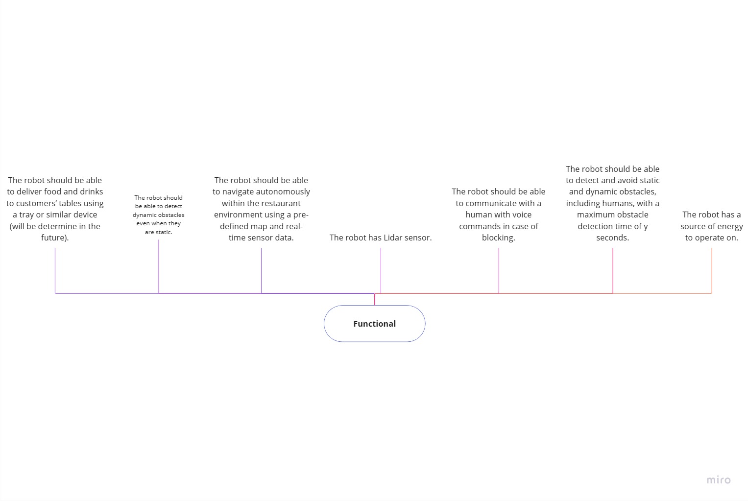

Requirements are a crucial part of the design process as they define the goals and constraints of a project. By establishing clear requirements, a team can ensure that their efforts are focused on achieving the desired outcome and that all necessary considerations are taken into account. In the case of the Restaurant Challenge, we took the system setting from the previous paragraph as well as challenge into account when designing the specifications for our requirements. This allowed us to develop a set of requirements that were tailored to the specific needs of the challenge. This allowed us to clearly define the capabilities and constraints of the robot, as well as the overarching goals of the challenge.
Our requirements included the ability for the robot to deliver food and drinks, detect dynamic and static obstacles, navigate autonomously using its sensors and a defined map in real-time, communicate with humans to avoid blocking, and avoid static and dynamic obstacles. The robot was also equipped with a lidar sensor and a source of energy.
Our requirements were divided into three groups: obstacle detection, safety, and reliability. For obstacle detection, the obstacles should be classified into dynamic and static obstacles. We specified that for every static object/obstacle detected within 0.7m range of the robot, it should plan a local path such that it avoids the obstacle and move along that local path. For every dynamic obstacle detected within the 0.7m range of the robot, the robot should send an audio command asking to move the dynamic obstacle away from the path, wait for some time until the object is moved and continue along the path. If the dynamic obstacle does not move within a certain amount of time, the robot should compute a local path to avoid the obstacle and move along that path. We did not specify the exact time to wait as it was an early process, and we could not estimate or know the exact computation overload.
For safety, we specified that the maximum speed of the robot should be undefined for the same reason, and that the minimum distance to static and dynamic obstacles should be different. The frequency of the lidar sensor should be updated at least at a certain frequency, such that it is sufficient to capture both static and dynamic obstacles.
For reliability, we specified that global and local path planners should be restricted by time constraints. The maximum delivery time should not exceed 10 minutes as this was given to us as an overall constraint.
By specifying our requirements, we were able to clearly define the capabilities and constraints of the robot, ensuring that our efforts were directed towards achieving success in the challenge.
Data Flow
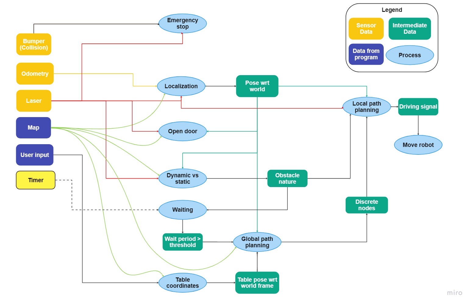
The diagram for data flow was created based on the available data to the robot from its environment through its sensors namely, the bumper data, laser data and the odometry data, as well as the known data from the map and the input table sequence. Each of these inputs were used in different segments of the code to generate intermediate data. The odometry and laser data were used to perform localization which in turn gives the pose (position and orientation) of the robot. The laser data was also used in the process of detecting obstacles and doors. This data is used further down the line in other processes like local and global path planning. Overall, the smooth transfer and interaction of data between each individual part of the code ensures that the robot moves in a predictable manner.

State Diagram
The state diagram describes how the code was to be split into segments. Firstly, the robot has to find its initial position using localization techniques as soon as the robot is turned on. Using the input form the user, we compute the global path which gives you the list of grids that must be traversed to reach a particular table. Once the path is established the local path planner takes in the list of grids one by one and performs local navigation. The local path planning ensures that the navigation between two grids is collision free.
If the path is blocked, we check whether is a door, a static or dynamic obstacle. In case it encounters a door or dynamic obstacle, the robot will request path access. If the local path planner is unable to find a clear path after certain waiting time, the map is updated and a different global path is found, which is then sent to the local navigator to reach the next table. If the table has been reached, the robot will orient itself towards it before announcing its arrival. From here the global path planning takes over to find the path to the next table and the process repeats till the final table is reached. However, the state diagram shown in the figure had many flaws, as were pointed out to us at the mid-term presentation. The major one of which is the breaking of the loop at the Emergency stop state. For the final challenge, however, some of these states were deemed redundant and not a priority for adding into the code.
Implementation
First and foremost, it becomes imperative to provide the robot with some information about the environment in which it is to operate. This is achieved by taking the map inputs that can be as accurate to the real world as possible and discretizing them into occupancy grids. Using these occupancy grids, the robot navigates through the restaurant. The grids act as nodes in the A* algorithm and provide information about the occupancy status.
Map Creation
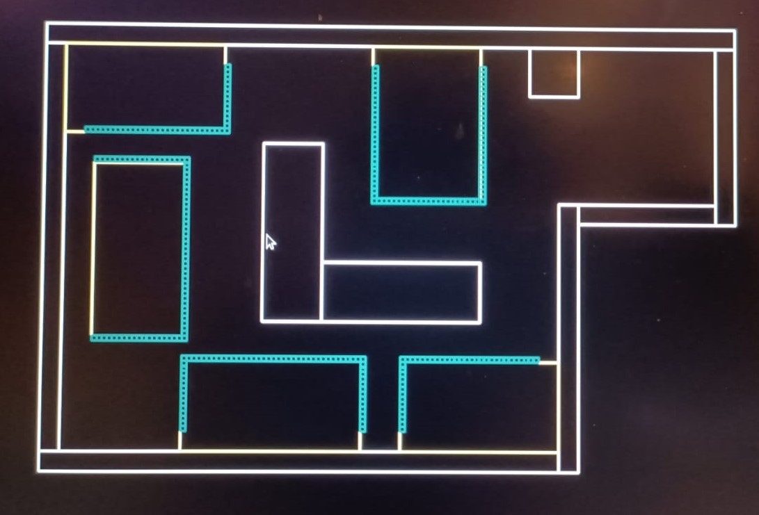
The need to automate reading the map data from a json file arose from wanting to create grids for the global path planning for navigation. The json file provided to the team contained the exact location in terms of x and y coordinates for each vertex of the tables and walls in the map and their corresponding vertex numbers (from here on referred to as nodes). The objects "tables", "walls", "doors" and "start area" also contained the connections between the nodes corresponding to their four corners. It was clear from the file that the total size of the restaurant was a 7m by 4.5m almost rectangular space as shown in the figure. At first, a "world" object was hardcoded into the json file that represents the outermost boundary of the map. Each of the objects were read from the json file and stored in different vectors.
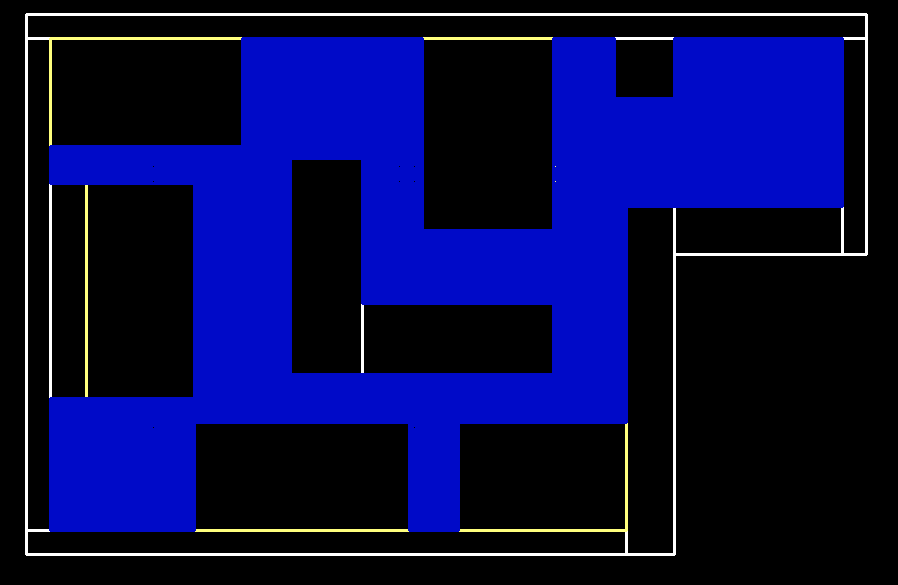
To ensure that the reachable grids are safe, the tables and the inner walls were blown up by 0.2m in all directions. The map was then discretized into grids of length 0.025m. All the grids that are inside the blown-up map objects, were made inaccessible to the global path planning. The remaining grid space was deemed open.
The occupancy grids contained in the door region, is marked by the "doorflag", which is true when the grid is inside the door region. Another member variable of the grid called "logodd" gives the likelihood of the grid being occupied.
Each grid possesses a variable that gives list of grids that are connected to it and are present in the open grid list.
A list of grids surrounding a table were chosen and linked to that specific table. These grids are the possible positions the robot can occupy to serve the table and were considered as the end goals for the global path planner.
All of these are utilized to execute the navigation of the robot.
The navigation process for mobile robots is categorized into four parts: global path planning, environmental mapping, obstacle avoidance and motion control. The global path planning determines the shortest route that the robot has to take from the start to the goal grid. As the robot traverses the global path, based on the laser data, the restaurant is mapped iteratively.
The open space approach is used to identify the heading direction of the robot, locally. Simultaneously, the artificial potential field created prevents collision with its surrounding objects, by computing the control inputs that ensures safety and eventually steers the robot to the goal grid.
Occupancy Grid Mapping
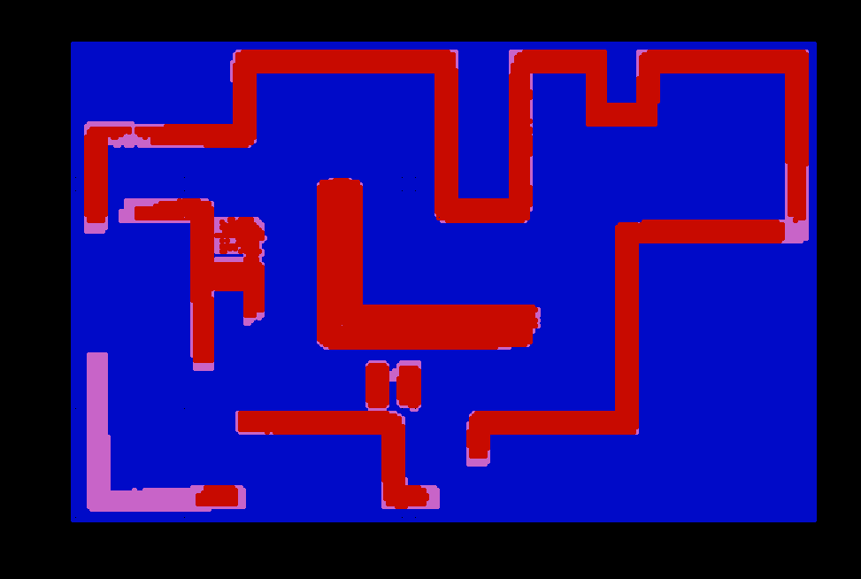
Initially the object detection was done using the logic that if the laser point hit an object within a scan radius of 0.7m, the corresponding grid was identified and updated as occupied such that local path planner can update it. However, there were few issues. As the grid size was decreased, the grids which fell inside the object and not on the periphery of the object were considered as unoccupied grids, although they were occupied in reality.
To overcome this, we decided to use occupancy grid mapping that represents the occupancy status of a grid based on the laser data, with a score called logodd value for each grid. This value is updated based on the laser hit points and the free space from the ray casting.
The new algorithm works as follows,
- All the grids that connect the current grid of the robot, to the hit point of each ray is computed using Bresenham's algorithm.
- The logodd value for the final hit point grid is increased by +1 while the intermediate grids are decreased by -0.5
- The logodd value is increased by +0.7 for clouds of grid up to 3 layers, that surround the hit point gird.
- The logodd value can take a maximum of +100 if the grid is occupied and a minimum of -100 if it is free
- Each grid is initialized with a logodd value of 5.
- Based on the final output of the logodd value, the likelihood of an object being present in that space can be computed. This was roughly plotted using the openCV package.
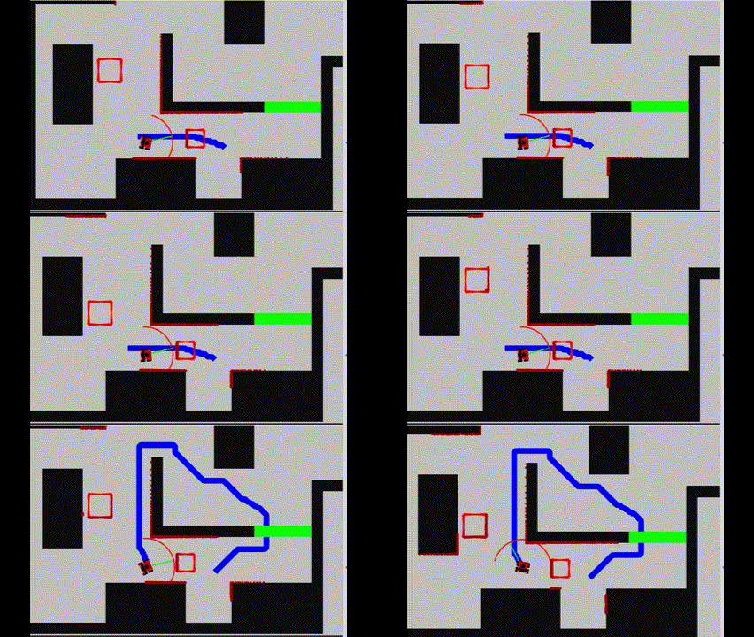
The A* algorithm is a widely used path planning algorithm for autonomous robots. Its importance to the challenge comes in the form of finding the shortest path between two points in the map. It calculates the cost to travel to a given grid and plans the path such that this cost is the least.
Firstly, based on the current position of the robot, the starting grid ID is obtained. Then closest grid associated to the table received as an input from the user, is determined from this grid. With these grid IDs as start and end IDs, the A* algorithm was implemented. These end IDs were also chosen based on the updated logodd values from the occupancy grid mapping algorithm.
This comes handy when the final goal is inside an object, in which case the A* algorithm is recomputed from the failure point.
The list of grids to reach the goal using the shortest path was found and sent to the open space algorithm. When node that is being sent has a logodd value more than the initialized value, the grids are skipped. If sufficient grids are skipped in the computed path, the path is forfeited and the A* algorithm is called again to calculate an alternate path from that position. After sending the grid ID's one by one the bot would reach that table with help of open space. After reaching that grid the start grid ID is updated to the previously reached ID and the goal is set as one of the grids in the cloud of grids surrounding the next table from the table sequence and then path was again computed. This process repeats until the final table is reached.
In order to obtain good navigation performance and accurate obstacle avoidance, it is necessary to have another type of navigation, namely local navigation that allows the robot to be truly autonomous in decision making in terms of moving to the next goal position.
Path following
The local path planner receives the list of grids that are to be reached one by one from the A* algorithm. If the grid that is destined is an intermediate grid, the local navigation is adopted until the bot is around a proximity of 0.5m. After reaching within this proximity the open space returns true to show it successfully navigated there. The next grid is then received, and this process is followed until the robot heads to the grid that is associated to the final point of the table. Here, the goal tolerance is set to 0.02m so that the robot reaches the table grid. After this the robot re-orients itself until it faces towards the center of the robot. Once this is achieved, the open space returns true to the A* algorithm to find the path to the next table.
Obstacle Avoidance
Open space
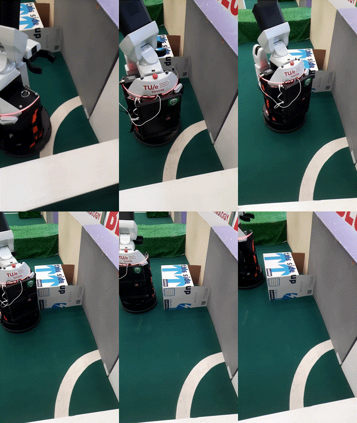
The obstacle avoidance is achieved using the open space approach and the APF. The open space provides an appropriate heading angle by scanning an area within a specific horizon limit, which was set to 0.7m in our trials. The radius of this scan is adaptive and decreases to the distance between the bot and the heading grid position. The heading pose is chosen based on the shortest point on the arc to the heading grid. This pose on the arc along with the scanned arc is sent to the APF to compute the control inputs for the bot.
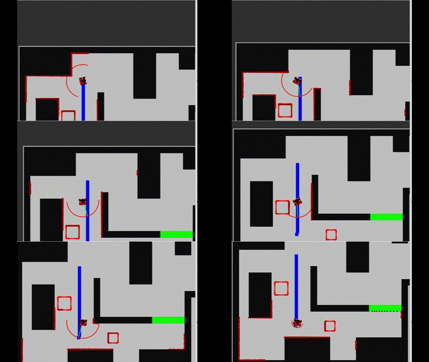
The point on arc is only chosen when the open arc is of sufficient length, i.e. wide enough for the bot to enter. If this is not possible, the robot temporarily marks these grids as blocked and sends false to the A* algorithm to recompute the global path.
Video link to the open space algorithm implemented on the robot in real time - https://tuenl-my.sharepoint.com/:v:/g/personal/a_nadig_student_tue_nl/EZhHaK7-WIZNsT-2XCIXlYkBclsjhFPy8pEfz20meuL0Dw?e=L1xeoy
APF
The position from the scan arc is received and an attractive potential function is defined using the norm of the distance. For the repulsive field, the closest hitpoint from the laser is obtained and the norm of this distance from the bot is used as the repulsive potential. They are combined together with a thresholding function on the repulsive potential such that it de-activates when the bot is sufficiently far away.
V_attractive = 0.5 ||x - x*||^2, where x denotes the 2D column vector of the robot, x* denotes the heading position received from the open arc.
V_repulsive = 0.5 ||x - x_hit||^2, where x denotes the 2D column vector of the robot, x_hit denotes the closest hit point of the laser.
S(x) = kx/(1+kx) - Thresholding function.
Final potential: V = V_attractive / S(V_repulsive); The gradient of this is used as the control input which is converted to robot as linear and angular input based on the holonomic constraints of the bot.
Encountering a door
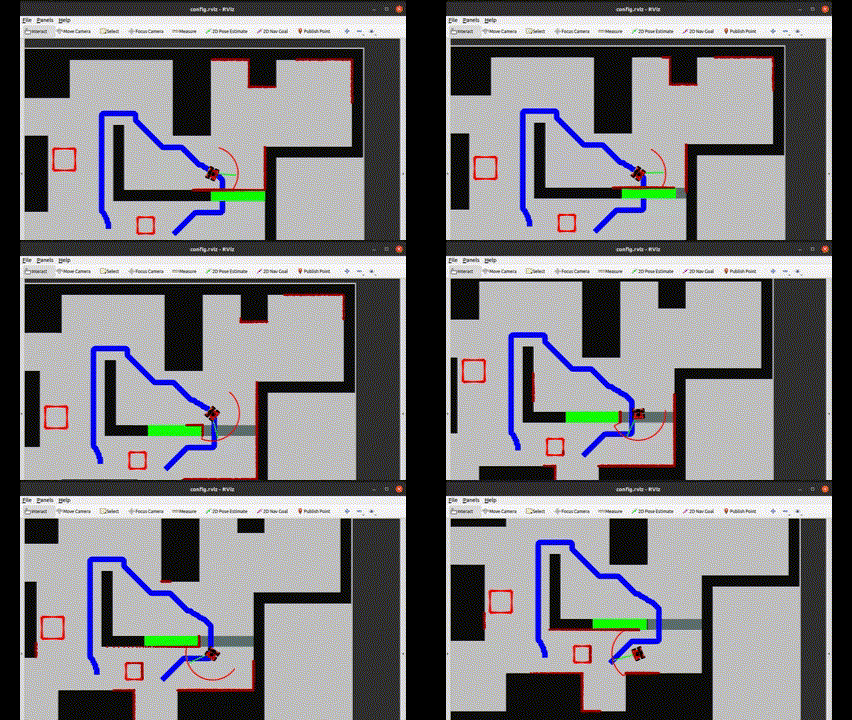
If the next grid is inside a door, we check if the door is opened or closed based on the logodd value obtained for the door grids. The door will be closed if the logodd values never decreased. If the logodd value for at least 20 grids inside the door is decreased, then the door is considered open and the loop returns to the open space. If it is declared as closed, a command "Open the door" is given, and waited for 5 seconds. If the door is not open (log odd never updates), it assumed that the door never opens and a global rerouting is done, by returning false to the A* algorithm.
Localization
Localization is an important aspect of autonomous navigation, as it allows a robot to precisely determine its position and orientation. In our approach to the Restaurant Challenge, we aimed to implement localization using a particle filter. This technique combines sensor measurements with a predetermined map, compensating for imperfections and adapting to real-world scenarios. However, implementing the particle filter proved to be more challenging than we anticipated. Our team was split and overloaded with multiple tasks, which resulted in a delay in finishing the particle filter assignment. Although we did manage to complete it, our attempt to transfer it to the robot at the last minute was not successful. As a result, we decided to focus our efforts elsewhere. For the final assignment, localization was done only with odometry data. While this was not our original plan, it allowed us to demonstrate the final challenge with uncertainties to the best of its capability.
Final challenge and discussion
Final challenge demo: https://tuenl-my.sharepoint.com/:v:/g/personal/a_nadig_student_tue_nl/EU3Z6S5qBgxOhPMEmV1KFAMBaRAe9SBfshWTYV_NrRqoBw?e=vZyf6i
Final challenge on simulator: https://tuenl-my.sharepoint.com/:v:/g/personal/a_nadig_student_tue_nl/EUpMwudeZNpPrkk9mcpjBloB8z0FDCiIgYUKVrZKdJjwwg?e=O2B6J3
For the same test case on simulator, we see that the bot successfully performed the task. However, the uncertain_odom was set to false. In the final challenge, we see that the bot never calls out that it arrived at table 1 and stops to recompute the global path over and over again. This is because the final goal grid was placed inside the table. This must not have occurred as the grids for the A* are always outside the blown-up map object. However, this could happen due to the localization error.
The bot was hard reset to initialize it's odometry frame at a specific point with respect to the world coordinate. This node placement went wrong either because this hard reset of the odometry frame was not accurate or because the error in odometry values was so erratic. However, on a separate test during the lab the robot reached the table 1 and started heading towards the table 4 after realizing the door was closed. (It recalculates the global path around. The door command was not implemented yet. )
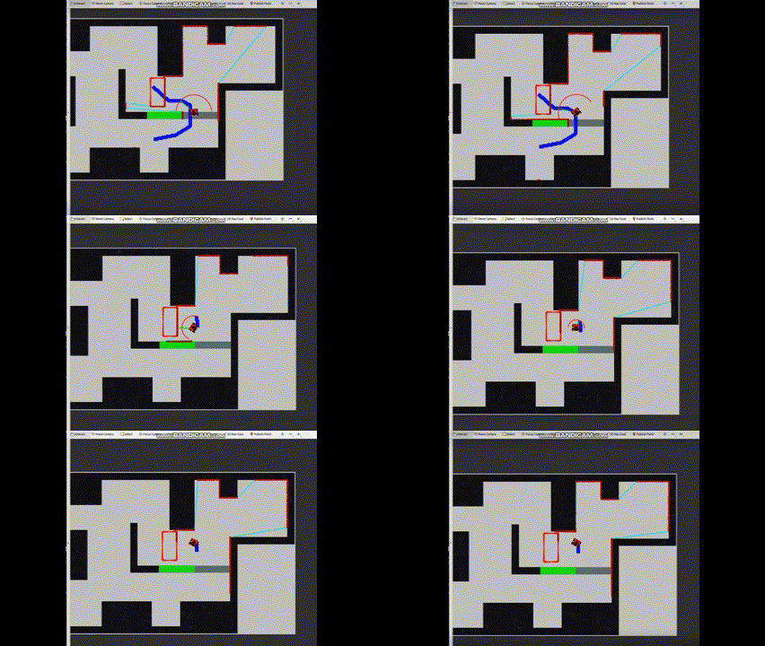
The video of the trial run - https://tuenl-my.sharepoint.com/:v:/g/personal/a_nadig_student_tue_nl/EXSxADxdQVZKrLB3dHxjgm8Bg_NyhwpqgLd4wIQ4qMbDGQ?e=5co8Mk
This video shows that the localization error was bearable and that the localization could not be the only failure point. The hard reset of the bot to initialize the odometry frame must have been offset. This could easily push the grid map off. Which is why the bot kept recomputing the global path.
Another argument that can be placed is that the path planning is capable of recomputing when the final goal is not reachable, i.e. within an unknown object. Nevertheless, this was not tested on the real bot, hence the robustness is uncertain. But this did not include the case when the final grid is inside map obstacle.
Finally, another result that we expected was that, the logodd updation. Since the front line of the table would be an unknown object for the bot, the logodds must be updated to a higher value, and the rerouting path must have given it a different path. But this was untested and if the start point was inaccurate along with inaccuracy in the orientation the algorithm would still miss the mark.
Conclusion and future scope
The final challenge was quite eye-opening in terms of seeing where the code was lacking.
As the team was stuck with the implementation of the localization of the robot, we were unable to fully complete the challenge. If the localization was executed and integrated into the code, our bot would have been able to deliver all the orders as well as avoid all the static and dynamic obstacles in its path.
A few more changes could be incorporated that the readability of the code could be improved. The closest grid to the table was calculated based on the pose of the robot. Instead, it could have been integrated in the A* algorithm.
Also, the gains of the velocities were very low which could also have been tuned to find the best suitable values.