Mobile Robot Control 2023 Group 15: Difference between revisions
| (7 intermediate revisions by 2 users not shown) | |||
| Line 146: | Line 146: | ||
*'''Why do we need to inject noise into the propagation when the received odometry information already has an unknown noise component.''' | *'''Why do we need to inject noise into the propagation when the received odometry information already has an unknown noise component.''' | ||
<br /> | ''This noise is necessary to compensate expand the amount of possibilities and poses for the robot to be in. This way the true uncertainty of the model can be represented.''<br /> | ||
*'''What happens when we stop here, and do not incorporate a correction step?''' | *'''What happens when we stop here, and do not incorporate a correction step?''' | ||
''This correction step is required for accurate assignment of weights to the particles based on actual measurement data. Thus in order to et an accurate and relatively certain pose estimate this step is crucial.'' | |||
| Line 155: | Line 157: | ||
*'''What does each of the component of the measurement model represent, and why is each necessary.''' | *'''What does each of the component of the measurement model represent, and why is each necessary.''' | ||
<br /> | ''The measurement model consists of 4 main parts:'' | ||
*''Local Measurement Noise: The model accounts for inaccurate sensor measurements by modelling a probability distribution around the true measurement. This is required since sensor readings are never perfectly accurate and include random variations.'' | |||
*''Unexpected Obstacles: This measurement model consists of an exponential distribution that allows the particle filter to estimate the pose of the robot in the presence of unexpected obstacles which are not incorporated into the original map.'' | |||
*''Failures: Since the sensor sometimes errors in the measurements it is important to model these failures by preventing them from negatively influencing the robot's state estimate. This model consists of a uniform distribution.'' | |||
*''Random measurements: This model consists of a uniform probability distribution and should be incorporated to maintain a robust estimation of the pose of the robot. Sometimes, there is no sensor measurement available and a random measurement model is required to continue with the estimation of the pose of the robot.''<br /> | |||
*'''With each particle having rays, and each likelihood being , where could you see an issue given our current implementation of the likelihood computation''' | *'''With each particle having rays, and each likelihood being , where could you see an issue given our current implementation of the likelihood computation''' | ||
''The likelihoods are multiplied with one another, meaning that as soon as one of the likelihoods is low this will decrease the entire uncertainty drastically such that it is perceived as zero likelihood.'' | |||
Assignment 5: | Assignment 5: | ||
| Line 165: | Line 172: | ||
*'''How accurate is the implemented algorithm?''' | *'''How accurate is the implemented algorithm?''' | ||
<br /> | ''In case of 2500 particles the Particle filter is very accurate. It is however important to get a good estimate of the initial pose. If this is the case, the particle filter shows very good estimates of the actual robot pose.''<br /> | ||
*'''What are strengths and weaknesses?''' | *'''What are strengths and weaknesses?''' | ||
''Strengths are that the pose is very accurate and the odometry drift is fully compensated for. This is no longer a problem. Weaknesses are that many particles are necessary for really accurate pose estimates which leads to longer computation times. Lastly if the initial pose is not estimated correctly everything will be propagated wrongly and error will be multiplied with error.'' | |||
Latest revision as of 10:35, 5 July 2023
Group members:
| Name | student ID |
|---|---|
| Tobias Berg | 1607359 |
| Guido Wolfs | 1439537 |
| Tim de Keijzer | 1422987 |
Practical exercises week 1:
1. On the robot-laptop open rviz. Observe the laser data. How much noise is there on the laser? What objects can be seen by the laser? Which objects cannot? How do your own legs look like to the robot.
The laser data shows with point clouds highlighted in red where objects are. In a constant environment the laser data is still quite fluid and dynamic. This indicates that there is significant noise on the robot. As of our own legs, they are visible as two small rectangles.
2. Go to your folder on the robot and pull your software.
This has been done.
3. Take your example of don't crash and test it on the robot. Does it work like in simulation?
After significant tweaking and updates, yes the simulation works.
4. Take a video of the working robot and post it on your wiki.
Video: https://youtu.be/FXOC3232ob8

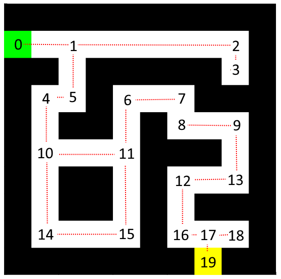
To improve the efficiency of finding the shortest path through the maze, it is suggested to decrease the number of nodes. By reducing the number of nodes, the algorithm will have to evaluate fewer nodes, which will make it more efficient.
The number of nodes can be reduced by removing nodes that are between the nodes that represent a straight line in the maze, as illustrated in Figure 1. This method results in a maze with 19 nodes, and the connections between them are indicated by red dotted lines. It is important to note that the cost of the straight paths should be updated to match the original cost of the same path. For example, the path between node 1 and 2 in the maze of Figure 1 would have a cost of 6.
The code for the Navigation-2 assignment can be found in the group repository in Gitlab, within the folder "Navigation-2".
The idea behind the used approach is based on the Artificial Potential Field Algorithm. The laser-data of the robot is used to detect objects. When these objects are within a specified range of the robot, a vector from the object to the robot is created. This vector is inversely scaled based on the distance of the object to the robot. In this approach local coordinates are used with the robot at the center of the coordinate frame. All the calculated vectors are stored in a list.
Coordinates for a goal are also defined. These are however globally defined, and are converted to local coordinates based on the odometry data of the robot. A vector from the robot to the goal is also drawn, this vector is however scaled to a fixed length, and not dependent on the distance of the robot towards the goal.
The list of vectors is summed to create a resulting force vector. Based on the orientation of this vector, the angular velocity of the robot is adjusted. The forward velocity is normally kept constant, however when the robot needs to make a very sharp turn, the robot decides to decrease the forward velocity and thus also decreasing it's turn radius.
This concept idea has resulted in the robot being able to solve the corridor maze on the simulator:
Video: https://youtu.be/9UnAluLiUOM
As well as that the robot is able to solve the corridor maze in real life during experimentation:
Video: https://youtu.be/Q__zXivK0Xg
Localisation Assignment 1:
Assignment 2:

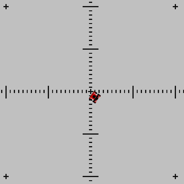
In order to determine the reliability of the odometry data in simulation, a map with distance markers was created as depicted in Figure 2. The map was used for a simulation in which the robot moved to four consecutive goals positioned on the map, forming a 5x5 meter box, and then returned to the starting point. The robot relied solely on the odometry data, employing an attractive force method derived from the artificial repulsive force code used in the navigation assignments. The code for the Localisation-2 assignment can be found in the group repository in Gitlab, within the folder "Localisation-2".
In the first simulation experiment, where the uncertain_odom option was not enabled, the robot successfully reached the goals and returned to the starting point, indicating that the odometry data was dependable for navigation.
Link to the video of simulation: https://youtu.be/e5O7nT2eaoo
However, in the second simulation experiment with the uncertain_odom option enabled, the odometry data proved to be highly unreliable. The robot failed to reach the designated goals on the map and deviated from the starting point by more than two meters.
Link of video of simualtion with uncertain_odom option: https://youtu.be/j7_fsJzvNnI
If the odometry data in real-life were as reliable as it was in the first simulated experiment, navigation could solely rely on this data. However, we are aware that this is not the case, and it would likely resemble the odometry data observed with the uncertain_odom option turned on due to sensor drift, slip of the wheels and other sources of error. Therefore, relying exclusively on odometry data for navigation would not be a suitable approach for the final challenge.
Assignment 3:

The experiment was replicated in real-life using the COCO robot. Although the disparity between the goals and the position obtained from the odometry data was not as significant as in the simulation with the uncertain_odom option, it still demonstrated a lack of reliability. The robot exhibited a deviation of approximately 40cm, whereas based on the odometry data, it should have stopped within 15cm of the origin, as illustrated in Figure 3.
Link to the video of the experiment: https://youtu.be/PfWP8JML4XE
Additionally, during the experiments, we encountered a case of robot kidnapping. When manually repositioning the robot to the origin, we noticed that the odometry data was not reset, resulting in further deviation from the expected path and goals.
Link to the video of experiment started after manual repositioning: https://youtu.be/pCS6CVaZp_k
Despite the smaller deviation observed, this experiment reinforces the conclusion that the odometry data cannot be considered sufficiently reliable for exclusive reliance in navigation.
Localisation Assignment 2:
Assignment 0:
- What is the difference between the ParticleFilter and ParticleFilterBase classes, and how are they related to each other?
There are two significant classes present in the ParticleFilter and ParticleFilterBase files. These two are identical to the file name. The ParticleFilter class is initialized by the ParticleFilterBase class, and uses prescribe base functions and expands on them. Thus the ParticleFilterbase class provides the standard functionality of particle filters, for example, it includes common functionalities like setting weights, and propagating particles. The ParticleFilter class can be initialized with both uniformly distributed particles and with a Gaussian distribution.
- How are the ParticleFilter and Particle class related to each other?
The ParticleFilter class uses instances of the Particle class to represent particles and perform particle filter operations. The Particle class provides the necessary functionality and data representation for individual particles within the particle filter algorithm.
- Both the ParticleFilter and Particle classes implement a propagation method. What is the difference between the methods?
The propagation method in the ParticleFilter class is responsible for propagating all the particles in the filter, based on the odometry data. The propagation method in the Particle class is used to update the state of an particle based on a given motion and an offset angle, taking into account the process noise.
Assignment 1:
- What is the difference between the two constructors?
The first constructor initializes the particle filter with 'N' number of particles, it calculates the weight of the particles and reserves memory for the vector in order to estimate a pose based on a uniform distribution. The second constructor additionally initializes the pose distribution parameters 'mean' and 'sigma' in order to estimate a pose based on Gaussian distribution with the mean and standard deviation parameters.

The second constructor, in addition to the above, initializes the pose distribution parameters, 'mean' and 'sigma', to estimate the pose based on a Gaussian distribution. The generated particles will be centered around the mean with a spread determined by the standard deviation.
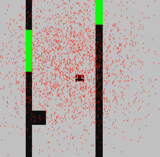
In Figure 4, a screenshot of demo1 is displayed, showing a Gaussian distribution of the particles surrounding the robot.
- What are the advantages/disadvantages of using the first constructor, what are the advantages/disadvantages of the second one?
The advantages of the constructor using uniformly distributed particles are simplicity and uniform coverage. This can be useful for exploring the entire state space. The main disadvantage is that a uniformly spread distribution is often not very realistic, leading to inefficiency in representing the true underlying distribution.
The constructor using Gaussian distributed particles offers advantages such as increased realism and efficiency. It can capture more complex patterns in the state space and focus on high-probability areas. Nonetheless, it comes with the disadvantages of increased complexity due to parameter estimation and sensitivity to inaccurate assumptions about the distribution.
- In which cases would we use either of them?
Overall, the choice between the two constructors depends on the specific requirements of the problem. The uniform distribution constructor may suffice for simple scenarios, while the Gaussian distribution constructor provides more flexibility and realism for capturing complex distributions and focusing on areas of interest.
Assignment 2:
- Interpret the resulting filter average. What does it resemble? Is the estimated robot pose correct? Why?
The filter average represents the robot state (position and orientation) estimation based on a weighted average of all the particles corresponding to a hypothesis of the robot state. Figure 5 shows the estimated robot pose in simulation. The orientation seems to be correct but the position not yet since the particles are initialized around the middle (0,0) of the map, the position which is currently indicated by the estimated pose.
- Imagine a case in which the filter average is inadequate for determining the robot position.
If there is a environment with multiple obstacles, the particle distribution may have multiple peaks, each corresponding to a possible location of the robot. In this case the filter average may provide a position estimate that is a weighted average of the peaks which may not accurately represent the robot's true position.
Assignment 3:
- Why do we need to inject noise into the propagation when the received odometry information already has an unknown noise component.
This noise is necessary to compensate expand the amount of possibilities and poses for the robot to be in. This way the true uncertainty of the model can be represented.
- What happens when we stop here, and do not incorporate a correction step?
This correction step is required for accurate assignment of weights to the particles based on actual measurement data. Thus in order to et an accurate and relatively certain pose estimate this step is crucial.
Assignment 4:
- What does each of the component of the measurement model represent, and why is each necessary.
The measurement model consists of 4 main parts:
- Local Measurement Noise: The model accounts for inaccurate sensor measurements by modelling a probability distribution around the true measurement. This is required since sensor readings are never perfectly accurate and include random variations.
- Unexpected Obstacles: This measurement model consists of an exponential distribution that allows the particle filter to estimate the pose of the robot in the presence of unexpected obstacles which are not incorporated into the original map.
- Failures: Since the sensor sometimes errors in the measurements it is important to model these failures by preventing them from negatively influencing the robot's state estimate. This model consists of a uniform distribution.
- Random measurements: This model consists of a uniform probability distribution and should be incorporated to maintain a robust estimation of the pose of the robot. Sometimes, there is no sensor measurement available and a random measurement model is required to continue with the estimation of the pose of the robot.
- With each particle having rays, and each likelihood being , where could you see an issue given our current implementation of the likelihood computation
The likelihoods are multiplied with one another, meaning that as soon as one of the likelihoods is low this will decrease the entire uncertainty drastically such that it is perceived as zero likelihood.
Assignment 5:
- How accurate is the implemented algorithm?
In case of 2500 particles the Particle filter is very accurate. It is however important to get a good estimate of the initial pose. If this is the case, the particle filter shows very good estimates of the actual robot pose.
- What are strengths and weaknesses?
Strengths are that the pose is very accurate and the odometry drift is fully compensated for. This is no longer a problem. Weaknesses are that many particles are necessary for really accurate pose estimates which leads to longer computation times. Lastly if the initial pose is not estimated correctly everything will be propagated wrongly and error will be multiplied with error.