Mobile Robot Control 2023 Group 9: Difference between revisions
| (10 intermediate revisions by 2 users not shown) | |||
| Line 21: | Line 21: | ||
#yes, it works the same as in the simulation as long as the speed is low enough and the distance is high enough. ie, the robot cannot move extremely fast (ie 0.7m/s) or stop too close to an object (ie 0.3m) with the real robot. | #yes, it works the same as in the simulation as long as the speed is low enough and the distance is high enough. ie, the robot cannot move extremely fast (ie 0.7m/s) or stop too close to an object (ie 0.3m) with the real robot. | ||
#https://photos.app.goo.gl/qFkDADTsP4tE5w4A8 (see video here) | #https://photos.app.goo.gl/qFkDADTsP4tE5w4A8 (see video here) | ||
<br /> | <br /> | ||
==Assignment 1:== | |||
[[File:Maze small.png|thumb|Maze Small with optimized node locations]] | |||
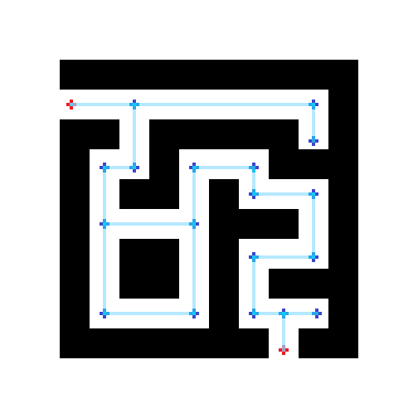
The nodes can be placed more efficiently by only placing nodes at places where there is a choice in directions. Numerous nodes placed one after another in a straight line require computation, but do not offer any added value to the system, since the only choice is to continue forward. In the Figure, red nodes are the start and end nodes, while dark blue nodes are the internal nodes. The light blue lines are all possible connections to follow. | |||
<br /> | |||
==Assignment 2:== | |||
We implemented an open space approach. This approach seemed best to us, as the majority of the other approaches required setting a goal, which seemed counter-intuitive due to the uncertain odometry of the robot. Using a look-ahead distance, and a looking angle, we searched for the longest range of angles that the robot could see uninterrupted further than or equal to the look ahead distance. Then we rotated the robot to move in that direction. | |||
===Simulations:=== | |||
Easy map: https://photos.app.goo.gl/CprLeQJM3VMo75UE6 | |||
Harder map: https://photos.app.goo.gl/hmdwc545hH43QAhB9 | |||
<br /> | |||
===Real Robot:=== | |||
Result: https://photos.app.goo.gl/8w9H96boxiLcTq5cA | |||
<br /> | |||
==Assignment 3: Localization 1:== | |||
[[File:Straight group9.jpg|thumb|Straight line experiment]] | |||
'''Part 1:''' The odometry data was successfully read by the script that was created. The current values for the x,y, and a data is printed, and the difference between the previous readings and the current readings are also displayed. [[File:Angle group9.jpg|thumb|Angular rotation experiment]]'''Part 2:''' The next step taken in this assignment is to compare the performance of the robot's odometry data. This is done by running a simple simulation in an empty hallway. The robot is driven forward and rotated using mrc-teleop, and the resulting odometry data is observed. This 'test' is ran two times, once with setting the uncertain_odom option to false, and once with true. When this setting was set to false, the robot was positioned in an upright position, meaning that driving forward would only impose changes to the x-data. The readings that were output were more or less accurate. Moreover, when the uncertain_odom was set to true, the robot did not start in an upright position, so driving forward would also impose a change in the x and y-data. This is due to the robot's coordinate frame is now askew when compared to the map's coordinates. However, the achieved data is still accurate. | |||
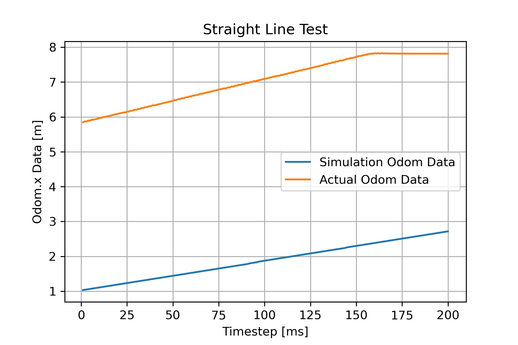
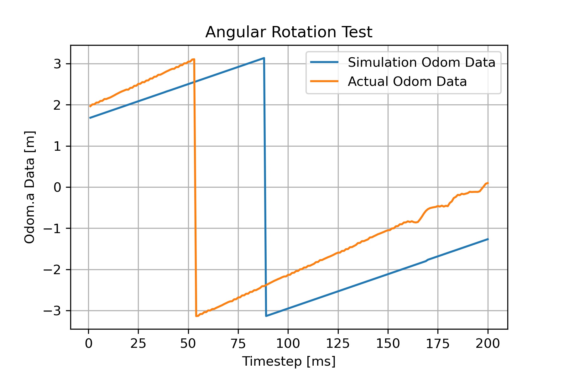
'''Part 3:''' The same procedure was ran on the actual robot and its behavior was observed. For the simulation and the actual experiment with the robot, we decided to save the odom data to a csv file. We ran two tests, one with just simply driving the robot forward, and the other with rotating the robot in one direction continuously using teleop. The collected data was then processed and graphed so we could compare this data visually. By simply inspecting the graphs visually, one can see that the slope for both, the x data and the angle data, were different for the simulation and the actual experiment. The slope for the actual tests was steeper, which confirms the fact that there is slippage affecting the robot. This can be seen in these two graphs: | |||
==Assignment 4: Localization 2:== | |||
===Assignment 0:=== | |||
*Particle.cpp makes the particles for the system, and ParticleFilter.cpp filters the particles based on odometry data & a resampling scheme. They work together to make & filter particles in the area. | |||
*For both of the classes, a propagation method is used based on the received odometry data. However, the ParticleFilter class then resamples based on this propagation, resulting in a change. | |||
===Assignment 1:=== | |||
*The first constructor is based on uniform distribution of the particles and the second is based on gaussian distribution of the particles. The advantages of the first one is that there is an equal chance of the robot being in any location of the map. The advantage of the second constructor is once you have a general idea of there the robot is, the distribution centers with a gaussian distribution around this area(s). | |||
*In the case that the robot is equally likely to start anywhere on the map, a uniform distribution is preferred. When it is known that a robot starts on one side/corner/room/area in the map, a gaussian distribution is preferred. | |||
===Assignment 2:=== | |||
*The filter resembles a cloud around the map origin, not around the robot. The robot estimation is not correct because there is no resampling done at this point in time. | |||
*The filter average may be inadequate for estimating the robot pose if there are obstacles like walls in the way. | |||
Latest revision as of 10:35, 26 May 2023
Group 9:
| Name | student ID |
|---|---|
| Ismail Elmasry | 1430807 |
| Carolina Vissers | 1415557 |
| John Assad | 1415654 |
Exercise 1:
dont_crash design: The idea was to move forward until an object is reached (0.5m within +/-45 deg) and then stop. If this object is removed, the robot should continue moving forward until it reaches another.
- Noise: it is there, and is slightly jittery. All objects at the height of the laser scanner are seen if they are not too far away (resulting in an inf range). If you walk near the robot, the legs look like lines that are oriented perpendicular to the robot.
- done
- yes, it works the same as in the simulation as long as the speed is low enough and the distance is high enough. ie, the robot cannot move extremely fast (ie 0.7m/s) or stop too close to an object (ie 0.3m) with the real robot.
- https://photos.app.goo.gl/qFkDADTsP4tE5w4A8 (see video here)
Assignment 1:

The nodes can be placed more efficiently by only placing nodes at places where there is a choice in directions. Numerous nodes placed one after another in a straight line require computation, but do not offer any added value to the system, since the only choice is to continue forward. In the Figure, red nodes are the start and end nodes, while dark blue nodes are the internal nodes. The light blue lines are all possible connections to follow.
Assignment 2:
We implemented an open space approach. This approach seemed best to us, as the majority of the other approaches required setting a goal, which seemed counter-intuitive due to the uncertain odometry of the robot. Using a look-ahead distance, and a looking angle, we searched for the longest range of angles that the robot could see uninterrupted further than or equal to the look ahead distance. Then we rotated the robot to move in that direction.
Simulations:
Easy map: https://photos.app.goo.gl/CprLeQJM3VMo75UE6
Harder map: https://photos.app.goo.gl/hmdwc545hH43QAhB9
Real Robot:
Result: https://photos.app.goo.gl/8w9H96boxiLcTq5cA
Assignment 3: Localization 1:

Part 1: The odometry data was successfully read by the script that was created. The current values for the x,y, and a data is printed, and the difference between the previous readings and the current readings are also displayed.

Part 2: The next step taken in this assignment is to compare the performance of the robot's odometry data. This is done by running a simple simulation in an empty hallway. The robot is driven forward and rotated using mrc-teleop, and the resulting odometry data is observed. This 'test' is ran two times, once with setting the uncertain_odom option to false, and once with true. When this setting was set to false, the robot was positioned in an upright position, meaning that driving forward would only impose changes to the x-data. The readings that were output were more or less accurate. Moreover, when the uncertain_odom was set to true, the robot did not start in an upright position, so driving forward would also impose a change in the x and y-data. This is due to the robot's coordinate frame is now askew when compared to the map's coordinates. However, the achieved data is still accurate.
Part 3: The same procedure was ran on the actual robot and its behavior was observed. For the simulation and the actual experiment with the robot, we decided to save the odom data to a csv file. We ran two tests, one with just simply driving the robot forward, and the other with rotating the robot in one direction continuously using teleop. The collected data was then processed and graphed so we could compare this data visually. By simply inspecting the graphs visually, one can see that the slope for both, the x data and the angle data, were different for the simulation and the actual experiment. The slope for the actual tests was steeper, which confirms the fact that there is slippage affecting the robot. This can be seen in these two graphs:
Assignment 4: Localization 2:
Assignment 0:
- Particle.cpp makes the particles for the system, and ParticleFilter.cpp filters the particles based on odometry data & a resampling scheme. They work together to make & filter particles in the area.
- For both of the classes, a propagation method is used based on the received odometry data. However, the ParticleFilter class then resamples based on this propagation, resulting in a change.
Assignment 1:
- The first constructor is based on uniform distribution of the particles and the second is based on gaussian distribution of the particles. The advantages of the first one is that there is an equal chance of the robot being in any location of the map. The advantage of the second constructor is once you have a general idea of there the robot is, the distribution centers with a gaussian distribution around this area(s).
- In the case that the robot is equally likely to start anywhere on the map, a uniform distribution is preferred. When it is known that a robot starts on one side/corner/room/area in the map, a gaussian distribution is preferred.
Assignment 2:
- The filter resembles a cloud around the map origin, not around the robot. The robot estimation is not correct because there is no resampling done at this point in time.
- The filter average may be inadequate for estimating the robot pose if there are obstacles like walls in the way.